Faculdade de Ciências
Departamento de Física
Numerical modelling in Transcranial Magnetic
Stimulation
Ricardo Nuno Braço Forte Salvador
Doutoramento em Engenharia Biomédica e Biofísica
2009
Faculdade de Ciências
Departamento de Física
Numerical modelling in Transcranial Magnetic
Stimulation
Ricardo Nuno Braço Forte Salvador
Thesis supervised by Prof. Doutor Pedro Cavaleiro Miranda
Doutoramento em Engenharia Biomédica e Biofísica
Aos meus pais e avós, sem o apoio dos quais não haveria tese. Em memória do meu bisavô Mário e da minha tia Rosa.
CONTENTS
PHYSICAL QUANTITIES ...V SYMBOLS AND ABBREVIATIONS ...VII ABSTRACT ... IX RESUMO ... XI ACKNOWLEDGMENTS... XVII
1 INTRODUCTION ... 19
-1.1 AIM OF THE WORK...-19
-1.2 OVERVIEW OF TRANSCRANIAL MAGNETIC STIMULATION...-20
-1.2.1 Basic principles and history ... 20
What is TMS? ... 20
History of brain stimulation with electromagnetic fields ... 22
-1.2.2 The electric field induced in TMS... 24
Two sources of the electric field ... 24
The quasistatic approximation... 25
Numerical modelling of the electric field... 27
-1.2.3 Fieldneuron interaction in TMS ... 30
Neuron’s membrane properties ... 30
Subthreshold and suprathreshold membrane response ... 31
Cable model and Cable equation... 34
Rattay activation function for TMS... 36
-1.2.4 Instrumentation... 37
Magnetic stimulators and pulse waveform ... 37
Coil design and optimization... 38
-1.2.5 Applications... 39
Different effects of TMS ... 39
Clinical applications... 40
Pathophysiology of movement disorders... 41
Therapeutic applications ... 41
Basic brain research ... 42
Animal studies... 43
-1.2.6 Safety ... 43
Induction of seizures ... 43
Other side effects... 43
-1.3 THEORETICAL OVERVIEW OF NUMERICAL METHODS...-44
-1.3.1 Calculation of the electric field: the finite element method ... 44
Introduction... 44
The method of weighted residuals... 45
The finite element mesh ... 47
Numerical methods for solving large linear systems... 50
-1.3.2 Numerical methods for neuronal modelling ... 52
Active compartmental models of neurons ... 52
Integration methods for the cable equation ... 54
-2 TMS OF DEEPLY LOCATED BRAIN REGIONS ... 59
-2.1 INTRODUCTION AND OBJECTIVES...-59
Problems when stimulating deep brain regions ... 59
Coil design optimization ... 61
External materials... 62
Objectives... 63
Published work... 64
-2.2 SIMPLE COIL DESIGNS: LOOP 1 AND LOOP 2 ...-64
-2.2.1 Methods ... 64
Head and coil models ... 64
High permeability core models ... 65
Numerical calculations of the electric field ... 67
Calculation of coil inductance... 68
Field focality ... 70
Coil inductance... 71
Primary component of the electric field ... 71
Secondary component of the electric field ... 74
Total electric field ... 76
Field focality ... 79
-2.2.3 Discussion... 81
Field induced by the loop 1 and 2 coil... 81
Effects of the use of ferromagnetic cores ... 82
Model limitations ... 83
-2.3 A REALISTIC COIL MODEL: THE H1 COIL...-84
-2.3.1 Methods ... 84
Head and coil models ... 84
High permeability core models ... 86
Numerical calculations of the electric field ... 86
Calculation of coil inductance... 87
Field focality ... 87
-2.3.2 Results ... 88
Coil inductance... 88
Electric field distribution... 89
Field decay ... 93
Field focality ... 95
-2.3.3 Discussion... 96
Field induced by the H1 coil ... 96
Effects of the use of ferromagnetic cores ... 96
Model limitations and future work ... 98
-3 FIELD – SINGLE NEURON INTERACTION IN TMS OF THE HUMAN MOTOR CORTEX... 101
-3.1 INTRODUCTION AND OBJECTIVES...-101
Mechanisms of neuronal activation on TMS... 101
The human motor cortex ... 104
TMS of the motor cortex... 106
Objectives... 109
Published work... 110
-3.2 IMPORTANCE OF TISSUE HETEROGENEITY ON NEURONAL ACTIVATION DURING TMS ...-111
-3.2.1 Methods ... 111
Volume conductor model and electric field calculation ... 111
Calculation of the neuronal response to the induced electric field ... 112
-3.2.2 Results ... 114
Electric field along the axon... 114
Axon’s response to the applied electric field... 114
-3.2.3 Discussion... 116
Influence of tissue heterogeneities on the induced electric field ... 116
Stimulation thresholds... 116
Significance... 117
-3.3 MODELLING TMS OF THE HUMAN MOTOR CORTEX...-118
-3.3.1 Methods ... 118
Sulcus model ... 118
Temporal waveform of the electric field ... 120
Types of neurons modelled ... 121
Electrophysiological and morphological properties of the modelled neurons ... 122
Numerical solution of the discretized cable equation ... 123
-3.3.2 Results ... 123
Electric field along neurons... 123
Activation sites and mechanisms... 127
Influence of pulse waveform and current direction on activation thresholds ... 129
Effects of tissue heterogeneities on activation sites and thresholds... 132
-3.3.3 Discussion... 132
Mechanisms of stimulation and site of activation ... 132
Interpretation of experimental results... 134
Model limitations and future work ... 136
-4 TMS OF SMALL ANIMALS ... 139
-4.1 INTRODUCTION AND OBJECTIVES...-139
Importance of coil size / brain size ratio... 140 Field focality ... 141 Objectives... 142 Published work... 142 -4.2 METHODS...-142 Mouse model... 142
Coil geometry and orientation... 143
Electric field calculation... 145
Assessment of coil performance... 146
-4.3 RESULTS...-146
Distribution of the primary electric field... 146
Distribution of the total electric field ... 147
Field’s magnitude and decay along test lines ... 150
Field’s focality ... 152
-4.4 DISCUSSION...-155
Cause of the low induced electric field ... 155
Performance of the different coil orientations ... 157
Model limitations and future work ... 158
-5 CONCLUSIONS ... 159
-5.1 SUMMARY OF MAIN FINDINGS...-159
TMS of deeply located brain regions ... 159
Fieldsingle neuron interaction in TMS of the human motor cortex ... 160
TMS of small animals ... 161
-5.2 LIMITATIONS OF THESE THEORETICAL MODELS...-162
Coil geometry... 162
Volume conductor geometry ... 163
Dielectric properties of tissues ... 164
Electrophysiological and morphological properties of neurons... 164
-5.3 THE FUTURE OF NUMERICAL MODELLING IN TMS...-164
-APPENDICES ...167
A QUASISTATIC APPROXIMATION ... 169
-A.1 FORMAL DEFINITION OF THE QUASISTATIC APPROXIMATIONS...-169
-A.2 GENERAL FORM OF THE EQUATIONS...-170
-A.3 QUASISTATIC FORM OF THE EQUATIONS...-171
-B VALIDATION OF NUMERICAL CALCULATIONS IN COMSOL ... 173
-B.1 COIL INDUCTANCE...-173
-B.1.1 Introduction ... 173
Inductance of circular loops ... 173
Inductance of toroids... 174
-B.1.2 Results ... 174
Inductance of circular loops: influence of the radius of the coil... 174
Inductance of circular loops: influence of the radius of the wire... 178
Inductance of toroids... 178
-B.1.3 Conclusions ... 180
-C ELECTROPHYSIOLOGICAL AND MORPHOLOGICAL PROPERTIES OF THE MODELLED NEURONS ... 181
-C.1 DISCRETIZED CABLE EQUATION...-181
-C.2 AXON MODEL USED IN TISSUE HETEROGENEITY STUDY...-181
-C.3 NEURON MODELS USED IN MOTOR CORTEX STUDY...-184
-D VALIDATION OF NUMERICAL METHODS USED TO SOLVE THE DISCRETIZED CABLE EQUATION ... 189
-D.1 IMPLEMENTATION OF THE ALGORITHM IN MATLAB...-189
-D.2 VALIDATION OF THE METHOD IMPLEMENTED IN MATLAB...-192
-D.2.1 Introduction ... 192
Comparison with NEURON... 192
-D.2.2 Methods ... 192
Specification of the model... 192
Implementation of the model in NEURON ... 195
-D.2.3 Results ... 196
Comparison of stimulation thresholds... 196
Comparison of the response of the transmembrane potential ... 199
Convergence rates ... 201
-D.2.4 Conclusion... 202
-Physical quantities
0
: Magnetic permeability of free space (4107H /m)
r
: Relative magnetic permeability of a medium
: Magnetic permeability of a medium ( 0r, []=H/m)
0
: Electric permittivity of free space (8.8541012F /m)
r
: Relative electric permittivity of a medium
: Electric permittivity of a medium ( 0r, []=F/m)
: Electric conductivity of a medium ([] = S/m)
: Charge density ([] = C / m3)
f : Frequency ([f] = Hz)
w: Angular frequency (w2 f , [w]=rad/s)
L : Inductance ([L] = H) C: Capacitance ([C] = F) : Resistance ([R] = ) R I : Current ([I] = A) E: Electric field ([E]V /m)
D: Electric displacement field ([D]C/m2)
B: Magnetic field ([B]T)
H : Magnetizing field ([H] A/m)
J: Current density ([J] A/m2)
: Scalar potential ([]V )
Symbols and abbreviations
AcPt: Action potential
aTES: Anodal Transcranial electric stimulation CSF: Cerebrospinal fluid
CT: X-ray computed tomography CTN: Corticospinal tract neuron DLPFC: Dorsolateral prefrontal cortex DV: Dorso-ventral
EEG: Electroencephalography EMG: Electromyography FEM: Finite element method
fMRI: Functional magnetic resonance imaging GM: Grey matter
GMRES: Generalized minimum residual method HPR: Half power region
LM: Latero-medial
LTD: Long term depression LTP: Long term potentiation M1: Primary motor cortex MEP: Motor evoked potential MRI: Magnetic resonance imaging MSO: Maximum stimulator’s output
PA/AP: Posterior-anterior / Anterior-posterior PET: Positron emission tomography
RL/LR: Right to left / Left to right RMT: Resting motor threshold
rTMS: Repetitive transcranial magnetic stimulation SI /IS: Superior-inferior / Inferior-superior
TMS: Transcranial magnetic stimulation WM: White matter
Abstract
In this work powerful numerical methods were used to study several problems that still remain unsolved in TMS.
The first problem that was studied is related to the difficulties that arise when stimulating sub-cortical deep regions with TMS, due to the fact that the induced field rapidly decays and loses focality with depth. This study’s approach to overcome this difficulty was to combine ferromagnetic cores with a coil designed to induce an electric field that decays slowly. The efficacy of this approach was tested by using the FEM to calculate the field induced by this coil / core design in a realistically shaped head model. The results show that the core might make this coil even more suited for deep brain stimulation.
The second problem that was tackled is related to the lack of knowledge about the dominant mechanisms through which the induced electric field excites neurons in TMS. In this work the electric field along lines, representing trajectories of actual cortical neurons, was calculated using the FEM. The neurons were embedded in a realistically shaped sulcus model, with a figure-8 coil placed above the model. The electric field was then incorporated into the cable equation. The solution of the latter allowed the determination of the site and threshold of activation of the neurons. The results highlight the importance of axonal terminations and bends and tissue heterogeneities on stimulation of neurons.
The third problem that was studied concerns TMS of small animals and the lack of knowledge about the optimal geometry, size and orientation of the used coils. This was studied by using the FEM to calculate the electric field induced in a realistically shaped mouse model by several commercially available coils. The results showed that the smaller coils induced fields with higher magnitude, better focality, and smaller decay than the bigger coils.
These results highlight the importance of numerical modelling in TMS, either in coil design, determination of basic neurophysiologic mechanisms or optimization of experimental procedures.
Keywords: Transcranial magnetic stimulation (TMS); Finite element method (FEM);
Resumo
A estimulação magnética transcraniana (TMS, do inglês Transcranial magnetic
stimulation) é uma técnica de estimulação neuronal não-invasiva cujo princípio de
funcionamento se baseia na lei de Faraday. Esta última estabelece que um campo magnético variável no tempo induz um campo eléctrico. Em TMS, o campo magnético é criado pela descarga rápida de uma elevada corrente através de uma bobina localizada próximo da zona que se pretende estimular. Por sua vez este campo induz um campo eléctrico, como estabelecido pela lei de Faraday. O campo eléctrico induzido em TMS coloca as cargas presentes nos meios intra e extracelular em movimento coerente o que, sob certas condições, provoca alterações no potencial de membrana dos neurónios afectados pelo estímulo, o que pode levar à geração de potenciais de acção. Dependendo da zona afectada pelo estímulo, a TMS pode dar origem a respostas fisiológicas diferentes, como contracções musculares no caso de estimulação do córtex motor. Têm também sido propostas várias possíveis aplicações terapêuticas desta forma de estimulação.
Desde a primeira aplicação com sucesso de TMS para estimular o córtex motor, atribuída a Anthony T. Barker em 1985, tem-se assistido a uma melhoria substancial do conhecimento acerca dos mecanismos físicos e fisiológicos subjacentes à técnica. Aliado a isso tem-se verificado uma optimização a nível de instrumentação, tanto no desenho dos estimuladores magnéticos como das bobinas de estimulação. No entanto, ainda subsistem limitações inerentes à TMS que permanecem por resolver, tanto a nível de instrumentação como a nível da compreensão dos mecanismos de funcionamento da técnica. O principal objectivo deste trabalho foi aplicar ferramentas de modelação numérica ao estudo de três problemas em aberto em TMS.
O primeiro problema que foi considerado relaciona-se com a estimulação de estruturas cerebrais sub-corticais localizadas profundamente. A estimulação destas estruturas tem-se tornado uma das áreas de investigação mais activas em TMS, uma vez que vários estudos apontam o seu papel nos mecanismos que medeiam a motivação e a recompensa, bem como nos mecanismos associados à depressão. No entanto, até à data, a TMS tem uma grande dificuldade em estimular regiões cerebrais profundas. A causa desta dificuldade prende-se com o facto da magnitude do campo induzido pelas bobinas tipicamente usadas, bobina circular e bobina em forma de oito, decair rapidamente com
a distância à bobina. Além disso, o campo tem também tendência a perder focalidade em regiões mais profundas, o que dificulta a estimulação precisa de uma dada região alvo. Nos últimos anos, os esforços têm-se focado no desenvolvimento de bobinas especialmente desenhadas para induzirem um campo que decai lentamente em profundidade. Um exemplo deste tipo de bobinas são as bobinas H, cujo formato faz com que estas induzam um campo que decai muito mais lentamente do que o induzido pelas bobinas usuais, mas à custa da focalidade do campo. Outros estudos têm apontado as vantagens da utilização de núcleos ferromagnéticos como forma de aumentar a magnitude do campo eléctrico e melhorar a sua focalidade. Estes núcleos, no entanto, têm até agora sido unicamente aplicados a bobinas com formatos tradicionais. Neste trabalho usou-se o método dos elementos finitos para estudar os efeitos da inclusão de núcleos ferromagnéticos numa das bobinas H, mais precisamente a bobina H1. Esta última foi desenhada para estimular estruturas localizadas sobre o hemisfério esquerdo em regiões pré-frontais dorso-laterais e ventro-laterais, com os neurónios orientados na direcção posterior-anterior, e estruturas localizadas em regiões pré-frontais mediais e orbitofrontais, com os neurónios alinhados preferencialmente ao longo da direcção lateral-medial. Numa primeira parte do trabalho foi criado um modelo da bobina H1, colocada sobre um modelo homogéneo e isotrópico de uma cabeça com um formato realista. Na segunda parte do trabalho usou-se o método dos elementos finitos para calcular o campo eléctrico induzido pela bobina H1 sobre o modelo realista da cabeça em três casos diferentes: bobina sem núcleos ferromagnéticos, bobina com um núcleo sobre o hemisfério esquerdo e bobina com um núcleo sobre a região frontal da cabeça. Em geral, a presença dos núcleos ferromagnéticos contribuiu para um aumento da magnitude da componente do campo eléctrico predominante na zona mais próxima do núcleo: posterior-anterior, no núcleo lateral, e lateral-medial, no núcleo frontal. Os núcleos também causaram um decréscimo do decaimento do campo ao longo do eixo superior-inferior. Contudo, o decaimento ao longo de outras direcções – direcção lateral-medial para o núcleo lateral e direcção anterior-posterior para o núcleo frontal – aumentou. Quanto à focalidade, a presença do núcleo frontal levou a uma diminuição da área estimulada, enquanto que o núcleo lateral aumentou a mesma. Os resultados sugerem que a presença dos núcleos pode melhorar algumas das propriedades do campo induzido pela bobina H1, tornando-a mais optimizada para estimulação de regiões localizadas profundamente. No entanto, face aos diferentes efeitos das duas posições
testadas para o núcleo, o posicionamento ideal terá sempre que levar em consideração a posição da região que se pretende estimular.
O segundo problema que foi estudado neste trabalho está relacionado com a falta de conhecimento acerca dos mecanismos precisos de interacção entre o campo eléctrico induzido em TMS e os neurónios. Estudos in vivo e in vitro têm ajudado a clarificar muitos dos possíveis mecanismos através dos quais o campo eléctrico estimula os neurónios. Regra geral esses estudos confirmam os resultados da teoria do cabo clássica que mostra que os neurónios são despolarizados (ficam com excesso intracelular de carga positiva) nas zonas onde é negativo o gradiente, ao longo do neurónio, da componente do campo induzido, na direcção do neurónio. Esses estudos também confirmam os resultados teóricos de que é possível obter estimulação mesmo em zonas onde o campo induzido é constante, desde que o neurónio termine ou dobre acentuadamente aí. Estes estudos, no entanto, não ajudam muito a clarificar os mecanismos dominantes no cérebro visto que, aí, os neurónios têm geometrias muito complexas e, como tal, existem muitos mecanismos possíveis de estimulação. Para tornar a situação ainda mais complexa, os resultados da estimulação dependem também da presença de heterogeneidades no meio condutor, que podem provocar variações muito rápidas no campo eléctrico ao longo dos neurónios, da orientação da bobina e da forma de onda do pulso de estimulação. Para ajudar a clarificar esta situação, neste trabalho criaram-se modelos diferentes de meios condutores que incluíam linhas representando as trajectórias aproximadas de neurónios. Em seguida, usou-se o método dos elementos finitos para calcular o campo eléctrico induzido ao longo desses neurónios por uma bobina em forma de oito. O campo eléctrico foi posteriormente usado na resolução de uma versão discretizada da equação do cabo, usando métodos numéricos apropriados. Num primeiro estudo, o volume condutor usado consistia apenas num paralelepípedo dividido em duas metades com condutividades eléctricas diferentes. O neurónio modelado nesse caso atravessava a interface de separação entre os dois meios e, como tal, o campo eléctrico ao longo do neurónio apresentava uma descontinuidade na zona da interface, devido à acumulação de carga que aí ocorre. Essa descontinuidade foi suficiente para estimular o neurónio com intensidades de estimulação dentro dos limites de funcionamento dos estimuladores magnéticos actuais. Num segundo estudo, construiu-se um modelo simplificado do sulco central e modelaram-se neurónios nesse modelo de sulco que se pensam serem relevantes para estimulação do córtex motor: neurónios piramidais do tracto cortico-espinhal,
interneurónios corticais e neurónios piramidais de associação. Os resultados mostraram que os neurónios modelados foram estimulados preferencialmente nas terminações axonais (interneurónios corticais) e nas dobras axonais (neurónios do tracto cortico-espinhal). Contrariamente ao sugerido no modelo inicial, a estimulação nunca ocorreu na zona onde os neurónios atravessaram a interface entre a matéria cinzenta e a matéria branca. No entanto, a descontinuidade do campo provocada por essa interface influenciou o limiar de estimulação. Nestes estudos o efeito da forma de onda do campo eléctrico induzido foi também contabilizado, sendo que os pulsos bifásicos conseguiram, regra geral, estimular os neurónios com limiares mais baixos do que os pulsos monofásicos. Estes resultados são consistentes com alguns resultados experimentais obtidos em estimulação do córtex motor em humanos e são úteis na previsão dos tipos de neurónios que são recrutados.
Por fim, o terceiro problema a ser considerado relacionou-se com a estimulação de pequenos animais recorrendo à TMS. Estudos envolvendo pequenos animais, especialmente roedores, têm sido usados para determinar os mecanismos neurofisiológicos da estimulação magnética. No entanto, estes resultados não podem ser imediatamente extrapolados para humanos, visto que os diferentes rácios entre o tamanho da bobina e o tamanho da cabeça levam a que os efeitos da estimulação sejam substancialmente diferentes. Outra dificuldade é a falta de consenso acerca da geometria, tamanho e orientação ideais para as bobinas usadas nestes estudos. Para clarificar esta situação, neste estudo usou-se o método dos elementos finitos para criar um modelo homogéneo e isotrópico de um rato com uma geometria realista. Em seguida calculou-se o campo eléctrico induzido por várias bobinas, baseadas em modelos comerciais, com diferentes geometrias, tamanhos e orientações. Os resultados mostraram que o campo resultante da acumulação de carga na interface entre a pele do rato e o ar diminuiu substancialmente o campo induzido pela bobina, além de aumentar o decréscimo em profundidade do campo. No que toca à focalidade do campo, analisada numa superfície representando o cérebro, esta melhorou muito devido ao campo causado pela acumulação de carga. Em termos da magnitude do campo induzido e do decaimento deste, as bobinas mais pequenas mostraram ser mais eficientes que as bobinas maiores. Estes resultados ajudam a prever procedimentos experimentais mais adequados para a estimulação de pequenos animais.
Os resultados obtidos nos três estudos efectuados mostram que técnicas de modelação numérica, como o método dos elementos finitos ou métodos de modelação de
neurónios, podem desempenhar um importante papel na optimização da instrumentação associada à TMS, no estudo dos mecanismos de interacção entre o campo e os neurónios e na optimização de procedimentos experimentais. O futuro da modelação numérica em TMS estará, então, assegurado e permitirá o desenvolvimento futuro da técnica, tanto no que toca a aplicações actuais como no que toca a possíveis aplicações futuras.
Palavras-chave: Estimulação magnética transcraniana (TMS, do inglês Transcranial
magnetic stimulation); Método dos elementos finitos (FEM, do inglês Finite element method); Modelação numérica; Modelação neuronal; Modelação do volume condutor.
Acknowledgments
Believe it or not, but it is not easy to write a PhD thesis! It is essentially an individual work, in the sense that only one person is actually writing it, but it simply isn’t possible without help from many other people. In this tiny space (only two pages) I will try to thank all the people that together made a huge contribution to this thesis.
My first words of acknowledgement go to my supervisor, Pedro Miranda, for all the support that he gave me in the last five years. He was the first to introduce me to the topic of magnetic stimulation and to the finite element method and to a number of fascinating topics that I will thoroughly discuss in the next 200 pages (give or take). More importantly than that, my supervisor is a person with whom it’s very easy to get along with, which made working with him all this years a true pleasure. I would also like to thank him for the patience he had in reading work after work time after time... I would also like to thank professor Eduardo Ducla-Soares, for it was him that first introduced me to the fascinating topic of Biophysics and Biomedical Engineering and guided my early studies in these fields. He also introduced me to IBEB and kept encouraging me through all this work.
Part with this work was developed in collaboration with Abraham Zangen and Yiftach Roth. I would like to thank their support and the availability for discussion that they showed. Another part of this work was developed in collaboration with Peter Basser, to who I would also like to thank for the speed he always demonstrated in answering our e-mails.
I must also thank my fellow colleagues, Paula and Sofia, who, together with me, walked this hard path. Sofia, like me, worked in modelling this amazing technique that is TMS, while Paula studied a vastly inferior and underpowered technique (tDCS or something like that…). However, they both deserve my most sincere acknowledgements for, if it weren’t for them, this journey would’ve been a very lonely one. Curiously we all finished our thesis at about the same time, much to the dismay of our supervisor who had to read and review three thesis.
Working in IBEB has also been a fantastic experience. I say this not because of the building itself (although there’s nothing wrong with it) and certainly not because of the surroundings (IBEB is close to an awfully looking football stadium), but because of the people that work there: Beatriz (for all the patience she had with me), Nuno Matela and
Nuno Oliveira (with whom I had some important football discussions), Sandra (who gave me some useful tips about writing my thesis), Susana and Mónica (whose devotion to work served as an inspiration to me), Mai Lu (who I bothered with countless questions about Chinese history), Abeye (who endured along with me the harsh trial of a vegetarian meal), Pedro Almeida (who encouraged me in a time when I was feeling down), Alexandre Andrade (with whom I had some interesting political discussions) and countless others. These people created a calming and relaxing environment that increased my productivity at least two-fold.
I also thank my closest friends who helped me take my mind out of research: Marco (my PIC burning buddy from my dark times at IST), Rodolfo, Sandro and Jorge (my fellow Tropical Sardines and some of the worst poker players the world has ever seen…) and Fábio (with whom I discussed important manga topics).
Por fim eu gostaria de agradecer à minha família. Foram os seus membros que me continuaram a empurrar para a frente, apoiando-me nos tempos difíceis. É claro que os meus pais foram quem mais me apoiou, dando-me apoio incondicional e acreditando sempre em mim em alturas em que nem eu acreditava... Não posso exprimir por palavras o quão importante o seu apoio foi para mim.
Vale-de-Marmelos, October 5th, 2009
This work was funded by the Portuguese Foundation for Science of Technology under grant nº SFRH/BD/23537/2005. I would like to offer my sincere acknowledgments to FCT for this support. Without it, I and countless other students wouldn’t have an opportunity to take our PhD courses.
1
Introduction
In this initial chapter the main objectives of this work will be presented. Additionally this chapter will also present a brief theoretical overview of transcranial magnetic stimulation (TMS) as well as of the most important numerical techniques used in this work.
1.1 Aim of the work
Since the first reported successful stimulation of a human subject with TMS (Barker and Jalinous, 1985), the number of applications of this technique has increased greatly. Nowadays, it is used in several cognitive studies and it is being tested for the treatment and diagnosis of a variety of diseases. Our understanding of the basic physical principles of this technique and of its physiological effects has also greatly evolved since the early days, which allowed for several optimizations, both in the instrumentation and in the experimental procedures. Despite this, there are still some problems regarding the application of TMS that remain unsolved and there is a lack of knowledge about some of the mechanisms through which it works.
One of the problems is the fact that TMS struggles to achieve stimulation of sub-cortical deep brain structures, because the field induced by the coils used nowadays rapidly decays and loses focality with increasing distance from the coil. This has become an active research topic in TMS, especially since the appearance of several recent studies that seem to indicate that stimulation of some deep structures may play a role in the study of reward and motivation mechanisms, as well as on the treatment of drug resistant depressions.
Another area that is still not well understood concerns the activation of neurons in TMS. Several possible stimulation mechanisms have been thoroughly studied, but the
dominant mechanisms for each type of neuron in the brain that is affected by a TMS pulse is still not well known. This impairs our understanding of the results obtained when stimulating some areas of the brain such as the motor cortex.
Finally, there is a lack of knowledge regarding the effects of TMS on small animals, such as mice. This stems from the fact that these animals have very different head sizes and geometries when compared to humans. Therefore, for the same size, geometry and orientation of the coil, the field induced in a human head can be very different from the field induced in the head of a small animal. This diminishes the usefulness of studies conducted in these animals, given that the results cannot be promptly extrapolated to humans.
It was this work’s objective to study the three topics described above to try to increase the overall knowledge about the mechanisms through which TMS operates and to overcome some of its problems. To do so powerful numerical techniques were used to model the field induced during TMS and its effect on accurate models of neurons. The topics previously mentioned are discussed individually in three chapters of this thesis. Each chapter contains a detailed review of what is known about the topic it concerns, a description of the methods used to study the problem, and a summary of the main results that were obtained.
In the remainder of this chapter, a brief overview of TMS and of the numerical techniques used in this work will be presented. The objective of this brief introduction is to familiarize the reader with some important concepts that will become necessary in the following chapters.
1.2 Overview of transcranial magnetic stimulation
1.2.1 Basic principles and history
What is TMS?
TMS is a non-invasive brain stimulation technique that achieves stimulation by the rapid surge of a high current pulse through a coil located near the region of the brain to
be stimulated. According to Biot-Savart’s law, the time-varying current flowing in the
coil gives rise to a time-varying magnetic field1:
C r r r r l d t I t r B 0 3 ' ) ' ( ) ( 4 ) , ( 1.2.1.1where 0 represents the magnetic permeability of free space, I the current that flows in
the coil, r is the position vector of the point where the field is being calculated and 'r is
the position vector of the current point of integration along the coil. The integral is performed along the coil, in the direction of the current. With the magnetic stimulators used nowadays, the current in the coil can reach a value of more than 5 kA, giving rise to strong magnetic fields ranging from 1 - 4 T. The duration of the current and of the magnetic field is, however, very short, lasting less than 1 ms (Jalinous, 1998).
The time-varying magnetic field induces an electric field. This principle is known as Faraday’s law of induction, and can be expressed mathematically by one of Maxwell’s equations (Jackson, 1999): t B E 1.2.1.2
The electric field induced in TMS is very intense (typically 100 V/m in the brain, (Roth et al., 1991b)) and has the same duration as the magnetic field (less than 1 ms, (Jalinous, 1998)).
Even though the magnetic field gives its name to TMS, it is the induced electric field that leads to neuronal stimulation, by forcing the free charges in the intra and extracellular media of neurons into coherent motion, which may cause some of these neurons to become depolarized (excess of positive charge on the intracellular side of the membrane). If the depolarization reaches a given threshold the neurons can fire action potentials, which propagate to other neurons synaptically.
The TMS pulse can generate a number of different physiological responses according to the brain area over which the coil is placed over. One area often studied is the hand area of the motor cortex, the stimulation of which gives rise to contralateral hand muscle movements. However, TMS can also exert a temporary reversible disruptive effect on brain activity over a target area, which is called a “virtual lesion”. One example of such a “virtual lesion” is the inhibition of perception of a given visual
1 It is usually considered that Brepresents the magnetic flux density and not the magnetic field. The latter
usually refers toH . Throughout this work, however, the magnetic field will always be represented by
stimulus by a TMS pulse applied over the occipital cortex. It should not be inferred from these results that the effects of a TMS pulse are restricted to the stimulation site. Instead, studies that combine TMS with neuroimaging techniques such as functional magnetic resonance imaging (fMRI) (Bohning et al., 1998) or positron emission tomography (PET) (Paus et al., 1997), show that the effect propagates into connected and functionally coupled areas, including sub-cortical brain regions.
History of brain stimulation with electromagnetic fields
The history of TMS cannot be dissociated with the history of electromagnetism or bioelectric phenomena. The first reports (4000 B. C.) of bioelectric events come from ancient Egypt, and describe the catfish that, if caught by a fishermen’s net would generate electric shocks forcing the fishermen to release the entire catch. Much later (47 A. C.), the roman philosopher Scribonius Largus recommended the use of another electric fish, the torpedo fish, as a cure for headaches and arthritis. Despite these early observations, it was not until the late eighteenth century, with the works of Galvani, that the subject of bioelectricity started to develop as a quantitative subject. Galvani discovered that when touching with a charged scalpel on the exposed femoral nerve of a dissected frog, violent contractions were elicited at the frog’s leg.
It was also around the late eighteenth century that the topic of electrostatics and magnetism underwent substantial development with the experiments of Cavendish (from 1771 to 1773) and Coulomb (published in 1785). In 1819, Oersted discovered that current flowing in a wire deflected a magnetic compass, and later, in 1831, Faraday noticed that when moving a coil through a stationary magnet, a current was induced in the coil, thus establishing that a changing magnetic field induced an electric field.
The first documented experiment of electrical brain stimulation was made in 1874 by Dr. Robert Bartholow, who injected current through two electrodes placed over the exposed dura of a patient. He discovered that current injection elicited contralateral limb movements.
Magnetic stimulation started developing as a subject in the late nineteenth century (1896), with the works of Jaques d’Arsonval who reported flickering visual sensations in a subject whose head was placed within a strong time-varying magnetic field. He called these visual sensations ‘magnetophosphenes’. Unaware of d’Arsonval’s work, Beer published in 1902 a paper also describing the induction of these
‘magnetophosphenes’ with a time-varying magnetic field. Soon after several researchers started to study the topic of ‘magnetophosphenes’ (see Figure 1.2.1.1 a), but it was not until 1946 with the work’s of Walsh and Barlow, that the site of stimulation was identified as the retina and not the occipital cortex.
Stimulation of nerves with time-varying magnetic fields was demonstrated for the first time by Kolin et al. in 1959, using a frog’s sciatic nerve. Later, in 1965, Bickford et al. were able to twitch skeletal muscles in intact rabbits, frogs and human subjects. In 1985, Barker and co-workers, working at the University of Sheffield, demonstrated a magnetic stimulator that was capable of achieving stimulation of the motor cortex of human subjects (Figure 1.2.1.1 b). They placed an excitation coil on the scalp over the motor cortex and recorded twitch muscle action potentials from the contralateral abductor digitii minimi using skin surface electrodes. From this first application of TMS, the potential clinical interest of this technique has continued to grow. This has leaded the Sheffield’s group to introduce the technique to a number of manufacturers. TMS stimulators (Figure 1.2.1.1 c and d) are now commercialized worldwide by several
companies, like Magstim (http://www.magstim.com), Magventure
(http://www.magventure.com/) or Nexstim (http://www.nexstim.com/).
Figure 1.2.1.1: (a) One of the first devices used to investigate the induction of ‘magnetophosphenes’ by Silvanus P. Thompson in 1910; (b) The first magnetic stimulator developed by the Sheffield’s group, attached to a circular coil; (c) and (d) Modern-day magnetic stimulators: Masgtim 200 stimulator and Magstim Rapid stimulator, respectively. Both stimulators are attached to a figure-8 coil (figures a and b taken from http://www.scholarpedia.org; figure c and d taken from http://www.magstim.com).
1.2.2 The electric field induced in TMS
Two sources of the electric field
As was already explained before, the time-varying current flowing through the coil gives rise to a time-varying magnetic field that, according to Faraday’s law, induces an electric field. As the electric field is the one that leads to stimulation of neurons, it is important to determine the spatial and temporal variation of this field. To do so, it is
convenient at this point to introduce the magnetic vector potential ( A), which relates to
the magnetic field according to the expression:
A
B 1.2.2.1
Substituting 1.2.2.1 into Faraday’s law (1.2.1.2) the following expression is obtained:
0 t A E
Because the curl of the gradient of a scalar function is zero (Jackson, 1999), the quantity within the curl in the previous expression can be written as a gradient of some
scalar potential:. Rearranging terms the following expression is obtained for the
total electric field induced in the brain during TMS:
t A E 1.2.2.2
Equation 1.2.2.2 expresses the electric field in terms of a magnetic vector potential and a scalar potential. Most importantly it shows that the electric field induced by TMS is
the sum of a primary component (At) and a secondary component ( ). Each of
these components can be given a physical meaning.
The primary component is the field that would be induced by the coil in a uniform isotropic medium such as air, if no conductive medium (head) was present. Under a set of approximations valid for the frequency range used in TMS, this field component depends only on the geometry of the coil and on the temporal waveform of the current’s time derivative.
The secondary component of the field results from charge accumulation at the boundaries that separate media with different electrical conductivities (e.g. the scalp / air interface or the white matter / grey matter interface). In order to understand why
charge accumulates at these interfaces consider that, at the latter, the normal component
of the current density ( ) must be continuous (Jackson, 1999): J
0 ).
(J1J2 n 1.2.2.3
Recalling that for a conductive medium such as the brain, the current density is given by , and that the primary component of the field is continuous across the interface (this field component depends only on the geometry of the coil), it is easily concluded that the only way to respect
E J
1.2.2.3 is that charge accumulates at the interface. This charge accumulation will increase the electric field at the medium with lower electrical conductivity and decrease it at the medium with higher electrical conductivity. This is illustrated in Figure 1.2.2.1. It should also be noted that charge accumulation only occurs if the primary electric field has some component perpendicular to the interface. This can be inferred from 1.2.2.3, which only involves the normal component of the current density and, thus, of the electric field.
Figure 1.2.2.1: Charge accumulation at the interface between two media with different electrical conductivities: 1 for the grey medium (bottom half) and 2 for the white medium (top half). The size of
the arrows is proportional to the value of the field’s component normal to the interface. The primary field (blue arrow) is continuous across the interface, whereas the secondary field (red arrow) increases the electric field in the medium with smaller conductivity and decreases it in the medium with higher conductivity. As a consequence, the total electric field (green arrow) is discontinuous across the interface, but the normal component of the current density (black arrow) is continuous. In this particular example 1>2; if 1<2 charge accumulation at this interface would be negative.
The quasistatic approximation
From the previous discussion it follows that finding a solution for the total electric field induced in the brain during TMS is equivalent to finding a solution for both the scalar and magnetic vector potentials. This task is simplified by applying the quasistatic approximation (Plonsey and Heppner, 1967; Roth et al., 1991a; Heller and van
Hulsteyn, 1992), which is valid for the range of frequencies of TMS pulses, from DC to 10 kHz according to (Miranda et al., 2003), and for typical dielectric properties of brain
tissues at those frequencies: = 1 S/m and r = 104 ( = 8.8510-8 F/m) (Roth et al.,
1991a).
The quasistatic approximation is actually a set of three approximations. The first approximation concerns propagations effects, which take into account the time required for changes in the source of a field (coil or charge in the tissue) to propagate to any other field point. In TMS, these propagation effects can be neglected if the wavelength of the electromagnetic field is much higher than the dimensions of the human head. Considering a value of 10 kHz for the frequency of a TMS pulse, the wavelength of the
field in the brain, 1/
f
, is of 300 m, a value much higher than any dimensionsassociated with the human body, which clearly demonstrates the validity of this approximation.
The second approximation consists in ignoring the capacitive effects of the brain tissue, considering the tissue essentially conductive. Under this approximation, the time that it takes for charge to accumulate at the boundaries between tissues with different conductivities is negligible. To check the validity of this approximation, Gauss’s law
( E ) can be combined together with the Continuity equation (J t)
to show that, inside any tissue the charge density () decays exponentially with a time
constant / . The ratio between this time constant and the duration of the stimulating
pulse gives a measure of the validity of this approximation: if the ratio is small, charge accumulates at a much faster rate than the frequency of the stimulating pulse. Using the same values as before for the frequency and dielectric properties of brain tissues, the
ratio between the two time constants is of the order of 10-3, which proves that this
approximation is valid.
The third and last approximation is to neglect skin-depth, i.e. the distance that fields can penetrate into tissues. In TMS, the externally applied magnetic field induces currents in brain tissues, which in turn induce their own magnetic field. These two sources of magnetic field tend to oppose each other, which causes the external field to decay as it penetrates into tissue. The distance along the tissue at which the field has already decayed to about 1/e of the field at the surface is called skin-depth (Cheng,
for the field induced in TMS is of 5 m, which again proves the validity of this approximation.
Under the quasistatic approximation, finding solutions for the scalar and magnetic potentials reduces to solving Laplace’s and Poisson’s equations (Cheng, 1989) for the scalar and vector potential, respectively (see Appendix A for a detailed proof):
1.2.2.4 0 2 coil J A 0 2 1.2.2.5
where Jcoilrefers to the current density in the stimulating coil. Equations 1.2.2.4 and
1.2.2.5 must be solved using the appropriate boundary conditions given by 1.2.2.3 and using the fact that the scalar potential must be continuous at the interfaces that separate media with different conductivities.
Laplace equation (1.2.2.4) is only valid for a homogeneous and isotropic medium. This is clearly not the case for the human head, because it contains several different kinds of tissues with different dielectric properties and because brain tissues also have anisotropic properties (Miranda et al., 2003). It is possible to generalize 1.2.2.4 so that it takes into account tissue anisotropy and heterogeneity (Miranda et al., 2003):
0 t A 1.2.2.6where represents the electrical conductivity tensor.
Numerical modelling of the electric field
The spatial distribution of the primary component of the electric field can be determined by solving 1.2.2.5 and requires knowledge about the geometry of the coil. It is possible to show (Cheng, 1989) that a general solution of 1.2.2.5 is given by:
' 0 ' ' ) ,' ( 4 ) , ( V coil dv r r t r J t r A 1.2.2.7where the integration is performed along the coil’s volume.
One way to calculate 1.2.2.7 is to represent each wire of the coil by a line (zero cross section) carrying a current I (Tofts, 1990; Grandori and Ravazzani, 1991; Roth et al., 1991a; Roth et al., 1991b; Miranda et al., 2003). Assuming this simplification, the volume integral in 1.2.2.7 reduces to a line integral around the coil:
Coil r r l d t I t r A ' 4 ) ( ) , ( 0 1.2.2.8Equation 1.2.2.8 has been solved analytically for a circular loop, using elliptic integrals (Cheng, 1989; Jackson, 1999). This model is very useful because it can be applied to all coil geometries that are composed of circular loops. One important example of the latter is the figure-8 coil, which consists of two circular loops located side-by-side and carrying currents flowing in opposite directions (Ueno et al., 1988).
Another method to calculate A that has been proposed (Roth et al., 1991a) is to
approximate the coil by a polygon and sum the vector potential induced by each side of the polygon. It should be mentioned, however, that approximating the wire by a line causes errors in the calculation of the vector potential especially in superficial regions close to the coil (Salinas et al., 2007). More complex models take into account the complete three dimensional geometry of the coil, by dividing each wire into several filamentary loops and solving 1.2.2.8 for each of those loops.
Once the spatial distribution of the vector potential is known, the primary component of the electric field can be found by finding the negative first temporal derivative of 1.2.2.8. As the only term in 1.2.2.8 that has a temporal dependency is I(t) it can easily be deduced that the primary component of the electric field is proportional to the first temporal derivative of the current on the coil. This also applies to the secondary component of the electric field, because the magnitude of the latter is proportional to the magnitude of the primary component. The temporal waveform of the electric field induced in TMS will be discussed in more detail in the ‘Instrumentation’ section.
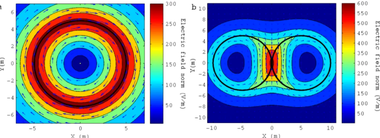
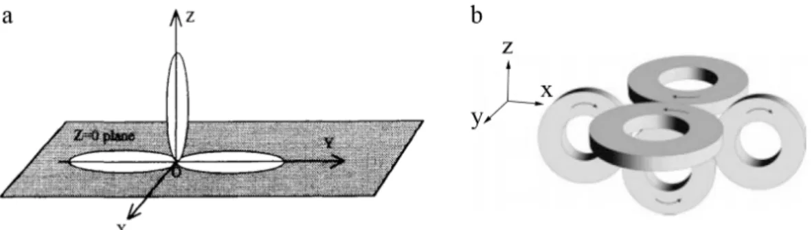
Figure 1.2.2.2 shows the norm of primary component (calculated using a theoretical expression, (Cheng, 1989; Jackson, 1999)) of the field for two coils traditionally used in TMS: the circular coil (a) and the figure-8 coil (b). The field is stronger under the coil windings and drops to zero in the centre of the loops and for regions far away from the coil. For the circular coil, the field only has an azimuthal component, whereas for the figure-8 coil, the field under the intersection of both sets of loops is oriented almost completely in the y direction. Under the figure-8 intersection, the field’s magnitude is maximum and almost double of the field’s magnitude under the circular coil.
Regarding the secondary component of the field, determining its spatial distribution requires solving Laplace’s equation for the scalar potential, 1.2.2.4. Unlike the calculation of the primary component of the field, which only requires knowledge about
Figure 1.2.2.2: Norm of the primary component of the electric field induced by a circular coil (a) and by a figure-8 coil (b). The direction of the field is indicated by blue arrows. The coils are centred in the xoy plane and the figures show the field for a plane 1 cm below the coil. The circular coil has a radius of 5 cm and 9 loops. The figure-8 coil is composed of two circular coils with similar properties to the one in (a). The coils are located side-by-side, separated by a gap of 1 mm. The field’s values were obtained for a fixed current’s rate of change of 100 A/s.
the geometry and orientation of the coil, for the calculation of the secondary component information about the geometry of the head and the dielectric properties of its different tissue types is also needed.
Initial studies performed with simple geometries (Tofts, 1990; Roth et al., 1991b; Eaton, 1992; Esselle and Stuchly, 1994) have all shown that the secondary component of the field greatly changes the total electric field. This is due to the fact that the secondary field reduces to zero the components of the total electric field perpendicular to the scalp’s surface (Roth et al., 1991b). The secondary field also affects, however, other components of the total field and increases its decay. This secondary component of the field is, therefore, of crucial importance when optimizing coils to stimulate deep brain regions, as will be discussed in more detail in Chapter 2.
More recently, the advent of faster computers and powerful numerical methods, such as the finite element method (FEM), has enabled the use of more realistic head models (Starzynski et al., 2002; Wagner et al., 2004; Chen and Mogul, 2009) and the investigation of the effects of tissue anisotropy and heterogeneity on the electric field (Miranda et al., 2003; De Lucia et al., 2007).
1.2.3 Field-neuron interaction in TMS
Neuron’s membrane properties
TMS stimulates neurons due to the force that the induced electric field exerts on the electric charges present both in the intra and extracellular medium. To understand why the charge movement leads to neuronal activation, it is necessary first to understand the basic properties of the neuron’s membrane.
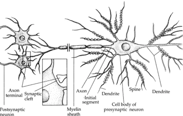
Neurons are very specialized cells of the nervous system. They are able to generate and propagate electrical signals, termed action potentials (AcPts). Patterns of these AcPts encode information within the nervous system. A neuron consists of a cell body or soma from which specialized processes called neurites arise (Figure 1.2.3.1). One of these processes is the axon, which usually conveys information away from the soma. The other processes are the dendrites, which transmit information to the soma. Axons have specialized endings, axon terminations, which come in close contact with regions of other neurons at synapses, where information is passed from one neuron to others. The axons of many neurons are covered by a myelin sheath except at regularly spaced gaps called Ranvier nodes. The myelin acts as an insulator and significantly increases the propagation speed of AcPts.
The ability of neurons to generate, propagate and transmit electrical signals is due to their highly specialized cell membrane. The latter contains ionic channels, which are transmembrane proteins that act as macromolecular pores in the cell membrane. These channels make the membrane permeable to ions that exist both in the intra and
extracellular media, most significantly sodium (Na+), potassium (K+) and chloride (Cl-)
ions. At rest, the concentrations of these ions in the intra and extracellular media differ,
the concentration of Na+ ions being higher in the extracellular medium and that of K+
ions being higher in the intracellular medium. Because the neurons’ membrane is permeable to these ions, they tend to flow through it pushed by the concentration gradient. This diffusion of ions causes charges of opposite sign to accumulate in the outer and inner membrane’s surface, which creates an electric field that influences the ionic charges diffusing through the membrane. If the cell membrane was permeable to only one ion, the voltage difference between the intra and extracellular cell membrane (transmembrane potential) would be such as to create an electric field that would oppose the diffusional forces. The membrane’s voltage at which equilibrium is attained is called
Figure 1.2.3.1: Schematic drawing of a neuron. This neuron receives input from several synapses at the cellular body and dendrites and establishes synapses with other neurons (postsynaptic neurons). The neuron has one axon and several dendrites. The unmyelinated first portion of the axon immediately after the cell body is called the initial segment. The dendrites have spines, which increase their synaptic area. (Adapted from (Martin, 1996)).
the Nernst potential. The values of the Nernst potential for each ionic specie differ from
neuron to neuron, but they are usually of the order of -88 mV, for K+ ion, and +61 mV,
for the Na+ ion (Malmivuo and Plonsey, 1995). A similar phenomenon happens in the
cellular membrane of neurons, for which the resting transmembrane potential varies from neuron to neuron between -40 mV and -100 mV (Hille, 1992).
In addition to containing these ionic channels, the lipid bilayer of cellular membranes separates the internal and external conducting solutions by a thin insulating gap, thus acting as a capacitor.
Subthreshold and suprathreshold membrane response
When current is injected into a neuron, either artificially via intracellular electrodes or as a response to a signal from another neuron, some of it spreads intracellularly to other areas of the neuron, and some of it flows through the membrane. The membrane’s current is the sum of two contributions: a capacitive term and an ionic term. The first one refers to charge that accumulates on both sides of the cellular membrane and charge
up the membrane’s capacitor, whereas the second term refers to the current that goes through the membrane’s ionic channels.
Early experiments have shown that depending on the magnitude of the injected current two different responses can be observed for the transmembrane potential. If the magnitude is below a given threshold, a subthreshold response is elicited, as shown in Figure 1.2.3.2. In this regime, the membrane acts as a parallel RC circuit, with the transmembrane potential initially increasing (depolarizing current pulse) / decreasing (hyperpolarizing current pulse) exponentially with time, reaching a given plateau and then, after the current stops being injected, decreasing also exponentially. This is a linear response, because the maximum value reached by the transmembrane potential has a linear relation with the magnitude of the injected current. In this regime, the ionic channels in the membrane can be modelled as resistors with a constant conductance. When the magnitude of a depolarizing current pulse is equal to or greater than a given threshold, a suprathreshold membrane response - action potential - is elicited (Figure 1.2.3.3). AcPts are rapid membrane responses that maintain a constant waveform and magnitude and that propagate without attenuation along the axon, contrary to what happens in the linear response, which decays spatially with distance from the site of current injection. The mechanisms behind the generation and propagation of AcPts were studied for the first time in the squid’s giant axon, but have been shown to apply to numerous other species and types of neurons. When the membrane depolarization reaches a given threshold, voltage gated sodium channels are activated, greatly increasing the permeability of the neuron to sodium ions, which enter the neuron pushed by the concentration gradient. This rapid sodium inflow accounts for the initial upstroke of the AcPt. Soon afterwards, the sodium channels start to become inactive thus decreasing the membrane’s permeability to this ion again and preventing the transmembrane potential from increasing further. Moreover, voltage gated potassium channels reach full activation after the sodium channels do. This leads to an outflow of potassium ions, which repolarises the transmembrane potential to baseline. The sodium current that enters the axon in the initial phase of the AcPt depolarizes adjacent axonal areas thus initiating the process there, which explains why AcPts propagate along a neuron. From the above description, it can be deduced that in order to account for suprathreshold responses, the ionic channels cannot be modelled as linear resistors. Instead, in this case, the conductance of the channels must be modelled by non-linear
Figure 1.2.3.2: Passive response of a neuron’s membrane. The figure in the left shows the electrical circuit equivalent to the membrane. C is the membrane’s capacitance and Rm its ionic resistivity. The
figure in the right shows the membrane’s response to a square current pulse of magnitude Is and duration Tdur. The transmembrane’s potential initially increases exponentially with a time constant RmC, reaches a
constant value proportional to the injected current and then starts to decay exponentially after the current stops being injected. (Adapted from (Malmivuo and Plonsey, 1995)).
Figure 1.2.3.3: Action potential recorded in a Ranvier node of a frog’s sciatic nerve at 14 ºC. The AcPt was elicited as a response to the square current stimulus shown below (Adapted from (Chiu et al., 1979)).
functions of the transmembrane potential.
Cable model and Cable equation
As was said before, the field induced in TMS influences the transmembrane potential. It is possible to quantify this interaction by assuming some simplifications, which will now be discussed. The first simplification is to consider that the neuron can be represented as a linear cylinder, representing the axon. This is not strictly necessary, for it is possible to extend this model to include the cellular body, dendrite, axon hillock and initial segment. Also, it is not necessary for the cylinder to be linear, as fibre tapering, bending and branching can all be taken into account. Other underlying simplifications of this model are (Roth and Basser, 1990): (i) to assume that the intracellular potential is only a function of the distance along the axon; (ii) to model the
axoplasm as an Ohmic linear conductor with conductance Ga and (iii) to neglect the
extracellular potential produced by the fibre’s own activity. The latter have been shown to be good approximations and are very often used in the literature (Roth and Basser, 1990; Basser and Roth, 1991; Nagarajan et al., 1993).
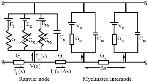
Under the simplifications assumed before and considering the membrane properties discussed in the previous sections, the axon can be represented as the linear network shown in Figure 1.2.3.4. The latter representation assumes that the membrane has been divided into smaller sections and that the membrane properties within those sections remain constant. In the case of myelinated axons, which is considered here, each Ranvier node is represented by one section and the myelinated internodes are divided into several sections, depending on the spatial resolution required. In this model, the circuit representing the membrane at the myelinated internodes only accounts for linear responses (parallel RC circuit), whereas in the circuit that represents the membrane at Ranvier nodes active responses are taken into account by modelling voltage gated sodium and potassium channels.
In the model constructed thus far, the axial current between point x and x+x of the discretized axon can be written as:
1.2.3.1
x x x x a a i x x G V x V x x G E s ds I ( ) ( ( ) ( )) ( )where V represents the transmembrane potential.
Figure 1.2.3.4: Electrical network representation of a myelinated nerve fibre. Ii represents the intracellular
axial current, Im the membrane current, x the length of the space step and Ga the total conductance of the
intracellular medium. The membrane is represented by a capacitor (Cn and Cm, represent the total
membrane capacitance at the Ranvier nodes and myelinated internodes, respectively) in parallel with several resistors, representing the ionic channels. The latter can have a constant conductance Gm in the
myelinated internode sections or conductances that vary with the membrane’s potential (GK, GNa) in
Ranvier nodes. At the myelinated internodes, the battery in series with the resistors (VR) represents the
membrane resting potential. At the Ranvier node, the batteries represent the Nernst potential of sodium (ENa), potassium (EK) and leakage (EL) currents.
term accounts for the effect of the field induced in TMS in the direction of the axon
(Ex). The difference between the axial current that goes out of a given node and the
current that goes into that node must be equal to the current that goes through the membrane, which is the sum of a capacitive component and an ionic current component:
) ( ) ( ) ( I x dt x dV C x Im m ionic 1.2.3.2
Hence, equating 1.2.3.2 to the difference between Ii(x+x) and Ii(x), given by 1.2.3.1,
the following expression can be obtained (Nagarajan et al., 1993):
x x x x x x x x a a ionic m ds s E ds s E G x x V x V x x V G x I dt x dV C ) ( ) ( )) ( ) ( 2 ) ( ( ) ( ) ( 1.2.3.3The cable equation (1.2.3.3) is actually a set of equations, one for each point of the discretized axon. Finding its solution requires knowledge about the total applied electric
models, this set of equations must be solved together with a set of equations that describe the behaviour of voltage gated ionic channels. Later on in this chapter several numerical algorithms suitable to solve these equations will be discussed.
In the case where only subthreshold membrane phenomena is of interest, taking the
limit of 1.2.3.3 when yields the following alternative version of the cable
equation (Roth and Basser, 1990):
0 x x E x V V t V x 2 2 2 2 ' ' ' 1.2.3.4
where V’ is equal to the membrane’s potential minus the membrane’s resting potential
and and are the space and time constants, respectively. It is possible to show
(Malmivuo and Plonsey, 1995) that the space and time constants are a measure of the spatial and temporal decay of the polarization caused by a given subthreshold stimulus.
Rattay activation function for TMS
If the neuron is initially at rest, no ionic current flows through its membrane and the transmembrane potential remains constant along it. Therefore, the cable equation reduces to:
x x x x x x x x a m G E s ds E s ds dt x dV C ( ) ( ) ( ) 1.2.3.5From the last equation it can be seen that if the term on the right hand side is positive, then the membrane will become depolarized by the electric field. On the other hand, if the same term is negative, then the membrane will become hyperpolarized. Given its ability to predict the polarization produced by the electric field, the right hand side of equation 1.2.3.5 is known as the activation function (Rattay, 1986).
A more traditional way to write the activation function takes advantage of the approximate form of the cable equation 1.2.3.4 (Roth and Basser, 1990; Nagarajan et al., 1993): x E S x 2 1.2.3.6
The activation function shows that the neuron’s membrane will become depolarized by
a TMS induced field when the spatial derivative of Ex in the direction of the neuron is
negative. However, as will be discussed further in Chapter 3, membrane polarizations can be induced even in regions where the field is homogeneous, provided that the