Urban Public Facility Location, Multipurpose
Trips and Spatial Competition
Equilibrium and welfare analysis
∗Didier Baudewyns
†January, 2001
Abstract
We study the impact of the urban location of one single public fa-cility on spatial competition à la Hotelling. If transportation costs are very low compared to the value of the public service then both firms tacitly choose the facility location without moderation of price com-petition, in contrast to mainstream results in the literature. In this event, minimum differentiation is efficient. For intermediate values of the relative transportation rate, inefficient partially-dispersed equilib-ria emerge with one firm at the facility site while its competitor locates at one end of the linear city. We also analyze the welfare impacts of changes, successively, in the facility location and the transportation rate, taking into account firms relocations.
JEL Classification: D43, L11, R32.
Keywords: public facility, multipurpose trip, full agglomeration, partial dispersion, optimal location.
∗I wish to thank Steffen Hoernig and Rui Nuno Baleiras for insightful discussion. †Universidade Nova de Lisboa, Faculdade de Economia, Travessa Estêvão Pinto
1
Introduction
It is generally admitted in the economic literature that competition à la Hotelling leads to inefficient spatial dispersion because sellers of homoge-neous goods differentiate their location in order to relax price competition. In this paper, we challenge this view from both the normative and the posi-tive viewpoints. Using the standard spatial setting, we will indeed show that homogenous duopolists may efficiently agglomerate without moderation of price competition if one takes into account two realistic features of urban life.
Firstly, it is a well-documented fact that people often make multipurpose trips, that is, they decide to visit a particular site for several reasons such as the purchase of various private commodities or the consumption of a local
public good1:
”For example, on the same trip, a consumer buys different goods, meet friends, visits a movie theater, goes to the post office, or just wanders and looks around. (...) The fact that consumers group their purchases in order to reduce travel costs creates de-mand externalities which firms would exploit by locating with firms selling other goods”. Fujita and Thisse (1999), p. 30.
Secondly, in many European city centres (e.g. Paris or London), a huge proportion of land is used by public facilities such as parks, museums, li-braries or major transportation nodes. As a result, some urban locations characterized by a large amount of public services around, may be more attractive for consumers, other things being equal. This may in turn give a demand externality-like advantage to any firm that would locate at these locations, especially when consumers desire to jointly consume both type of goods (public and private) on one single trip–or, in the case of a trans-portation facility, when the fixed cost of travel (waiting time, parking) is directly reduced.
The most casual observations suggest indeed that public facility sites often serve as agglomeration points for firms (see also Thisse and Wildasin, 1992). This is the idea developed in the next section. We will assume that one single public facility is located somewhere within the linear city before the standard location-then-price game à la Hotelling takes place. We will especially establish that for a very low transportation cost, or a high value the public service, minimum differentiation occurs at the facility site without any moderation of price competition.
As far as we know, the effects of spatial variation in the amount of public goods on urban location decisions made by oligopolistic firms are seldom an-alyzed, with the exception of Thisse and Wildasin (1992). The latter paper
1
examines the impact of the location of one single public facility on the inter-dependent locational choices of firms and households. Thisse and Wildasin (1992) mainly show that if the public facility is centrally-located then one obtains symmetric equilibria ranging from the fully agglomerated outcome (both firms at the facility central site) to the fully dispersed outcome where both firms are situated at opposite ends. On the other hand, if the public facility is situated close to one end of the city then any equilibrium exhibits
both firms at the center of the urban area.2
As compared with Thisse and Wildasin (1992), we want to relax the fixed price assumption by using the standard location-then-price game à la Hotelling. The idea behind is that price competition is a strong centrifugal force that could destroy the possibility of agglomeration at the facility site. Moreover, one objective of our paper is to depart from the assumption of independent trips by exploring the effect of multipurpose shopping on spatial competition–as suggested by Thisse and Wildasin (1995) themselves by the way.
The remainder of the paper is organized as follows. The following section presents the model. Section 3 solves the subgame in prices and section 4 characterizes all the equilibria of the location-then-price game. Section 5 analyzes the efficiency of the market outcomes. Section 6 looks at the effects of a change in the facility location on welfare, taking into account relocations of firms. Section 7 analyzes welfare implications of policies aiming at a decrease in transportations costs. Section 8 concludes.
2
The model
Our set-up closely follows the assumptions made by d’Aspremont et al (1979) (hereafter called AGT). Consumers are uniformly distributed along a linear city [0, 1] and bear a quadratic transportation cost. The population of con-sumers is normalized to one. As emphasized in the preceding section, we assume that one single public facility is located somewhere in the linear city, at some location denoted l ; without loss of generality, suppose that the
fa-cility is in the second half-segment: 12 ≤ l ≤ 1. We denote α > 0 the value of
the service provided by that facility to any individual. In order to focus on locational aspects, we assume that α is determined outside the model and
constant throughout the system.3 Two oligopolists, indexed i = A, B,
pro-duce a homogenous good or service at respective prices pi with an identical
marginal cost that is normalized to 0 (standard). As suggested by Thisse and Wildasin (1992), p. 85: ”as in Hotelling (1929)”, one can think of
”su-2
The idea is that there exists an equilibrium only if revenue is large enough, to such an extent that the market area effect dominates the consumption effect.
3
This is standard in the litterature (see ReVelle, 1987) and is in the spirit of Thisse and Wildasin (1992).
permarkets selling private goods on a large scale”. After having observed the location of the public facility, the two private firms play a game in two stages. In the first stage, they simultaneously choose their own location, respectively a and 1 − b ∈ [0, 1] with 1 − b − a ≥ 0 without loss of generality. The last stage is the standard Bertrand price competition.
As emphasized in the introduction, we now modify AGT by assuming that households have a preference for multipurpose ”one-stop” trips. Firstly,
assume that households bear some fixed cost of transportation denoted tf for
each trip they make (e.g. waiting time, parking). The remaining part of the
total transportation cost is quadratic in distance as in AGT: tf+ tz2 (tf, t >
0) is the travel cost incurred by a consumer who travels a distance z for the purpose of buying one unit of the private (or public) service. Secondly, the utility derived at location l depends on the value of the public service provided at that location. To make it clear, consider that firm B is located at the place of the public facility whereas A is not. Then, denoting u the value of the private good, the utility of the consumer residing at x is simply given by
U (x, a) = u − pA− tf − t(x − a)2 (1)
if she shops at A, or
U (x, l) = u − pB− tf − t(l − x)2+ α (2)
if she shops at B and consumes a quantity α of the public service.4 We now
give examples of public services we have in mind and the corresponding in-terpretation of the parameter α (the demand externality) in the specification above.
2.1
Example 1: major transportation node
Imagine that the ”public facility” at l is a major node of the urban trans-portation system. We can rewrite the utility derived from shopping at B when this firm is situated at l as
U (x, l) = u− pB− (tf − α) − t(l − x)2
Clearly, α represents the reduction in the fixed cost of travel due to bet-ter bet-terminal conditions (e.g. waiting time in public transit, or direct link
between the highway and the parking).5
4The reservation price u is large enough to ensure that every consumer is served in any
equilibrium. In fact, we checked that u > 3t is sufficient (standard).
5For example, in Lisbon, the hypermarket Continente lies (in the mall Colombo) right
next to the North-South highway with a direct access, from the highway, to the 20-entrance parking of the mall with space for 6800 vehicles; it can also be reached by two other avenues that cross there; on this site, there are also two taxi ranks, a metro station and a bus terminal served by 24 urban and suburban bus routes. It is important to notice that the building of the highway link and the extension of the metro at that location were the results of prior decisions made by the City Council of Lisbon.
2.2
Example 2: park, museum, etc. and ”one-stop”
multi-purpose trips
Assume now that α represents the quantity consumed of a public service provided by a facility such as a museum, a park, a post office, a library or any other government administrative buildings. Multipurpose ”one-stop” trips to location l are due to nonconvexities in the transport cost as captured by
tf in equations (1)-(2) above. Observe that preference for one-stop trips is
indeed very strong in our specification since those consumers visiting firm A do not decide to make a separate trip to the facility for the unique purpose of consuming the public good. This one-stop trip pattern emerges if the fixed component of the disutility of travel is large enough. In particular, it
should be clear that, for tf > α, no consumer will make an additional trip
to the facility.
In fact, some (or all) consumers may make independent trips to the facility but we assume that this occurs on ”another day of the week”. Indeed, the shopping behavior should be apprehended over one week or one month (see Stahl, 1987). Then, following Thill (1992), assume that households consume the private good at a constant rate and purchase it according to a fixed schedule: every Saturday, let us say, all households necessarily buy one unit of the private good (main shopping day) while in some intermediate day of the week, some consumers make one independent trip to the public
facility: they consume a quantity β > tf > α of the public good, let us
say, every Wednesday.6 The last inequality simply means that the marginal
utility of the public good is decreasing: this may be due to a more binding time constraint on Saturday (a high amount of time is already spent in the shopping activity, including storage at home and holding inventory, time
spent in the shop)7 or the fact that the public service has a higher utility
during the week (e.g. post office).8 Then, our model is unchanged since, for
these consumers, we simply add the same net utility β − t(l − x)2 to both
U (x, a) and U (x, b) in order to derive the weekly level of utility.9 It is readily
6Thus without shopping, on that day, a second unit at B, should that firm be located
near the facility. Clearly, if β > tf + t then all the population will indeed make an
independent trip to the facility during the intermediate day.
7
see Thill (1992), footnote 3.
8
Consider also the following example: on Saturday, some consumer shops at B in the Quartier Latin (central Paris) and, since the transportation cost is sunk, s/he decides to wander in the park ”Jardin du Luxembourg” ; or s/he might choose to visit a nearby museum. Assume also that every Sunday afternoon, our consumer systematically visits the same park with the family. Our specification expresses the idea that the net utility derived from the consumption of the public good will probably be lower on Saturday as compared to Sunday, because of different time constraints (obviously, as opposed to many retail firms in central Paris, parks and museums are open on Sunday). Due to the fixed cost of travel, those patronizing firm A on Saturday derive a higher weekly utility by visiting the park only on Sunday.
verified that, under the assumption β > tf > α, those consumers patronizing
firm A on Saturday are better-off when they split, both spatially and over the week, their consumption of both types of good, private and public.
To sum up, our utility specification captures the main idea that people have the opportunity to consume, on one single trip, an (additional) amount of the public service when they patronize the firm located in the vicinity of the facility. This is the standard ”demand externality” effect: shopping trips characterized by economies of scope in jointly buying independent goods on the same site induce demand complementarities which translates in an increase of the aggregate consumption of each good or service (see Stahl, 1987). It is convenient to let f (xi) = ½ α if xi = l 0 if xi 6= l (3)
where xi is the location of firm i (xi = a, 1 − b). The utility of a consumer
residing at x and shopping at firm i is then given by
U (x, xi) = u − pi− tf − t(x − xi)2+ f (xi) (4)
For expositional purpose let us denote the externality advantage of firm B as follows: ∆f (a, b) = f (1 − b) − f(a). It is equal to α (respectively −α) if only firm B (respectively only firm A) is at the place of the public facility ; it is equal to zero in any other case. From (4), the consumer who is indifferent
between the two marketplaces resides atx such thatb
b x = pB− pA 2t(1 − b − a)+ 1 − b + a 2 − ∆f (a, b) 2t(1 − b − a) (5)
When the two firms are located at the same point, we assume that consumers choose randomly between them so that the demand facing any firm is a
one-half share of the population (standard).10 We now can write the demand
for the product sold by firm i (i = A, B) as:
DA(pA, pB; a, b) = b x if 0 <x < 1, a 6= 1 − bb 0 ifx ≤ 0, a 6= 1 − bb 1 ifx ≥ 1, a 6= 1 − bb 1 2 if a = 1 − b (6) DB(pA, pB; a, b) = 1 − DA(pA, pB; a, b) (7)
Finally, respective profits are as follows:
Πi(pA, pB; a, b) = piDi(pA, pB; a, b) i = A, B (8)
two last utility functions.
1 0
3
Price competition
Following the backward induction principle, let us tackle the solution of the price game. For conciseness, let us drop the arguments a and b in any price (or profit) function for the rest of this section. Suppose also for the moment that each firm expects that it will face a positive demand at
dispersed locations. Then, for fixed locations, let Pi(pj) denote the best
response of firm i to a price pj set by its rival. The first-order conditions for
profit maximization lead to the following system of equations which must prevail in any equilibrium with positive demands:
PA(pB) = pB 2 + t(1 − b + a)(1 − b − a) − ∆f(a, b) 2 (9) PB(pA) = pA 2 + ∆f (a, b) + t(1 + b − a)(1 − b − a) 2 (10)
First, if both firms are ”outside the facility place” then the price subgame is identical to AGT: equilibrium prices are given by the solution of (9)-(10) where ∆f (a, b) = 0 [see Tirole, 1988, page 281, Eqs. (7.7)-(7.8)].
Second, assume that firm B is located at the public facility site whereas A is located somewhere on the left side (a < l). Whence, only those consumers patronizing firm B benefit from the provision of the public service: they get an additional level of utility ∆f (a, b) = α. In stark opposition to AGT, for low values of t relatively to α, the system of price functions above is simply not valid because it implies a zero-demand for the firm situated outside the
facility location, even if the latter firm prices at marginal cost.11 On the
other hand, for a high value of the ratio t/α, the pair of equilibrium prices is the solution of the system of first-order equations above:
Result 1. Assume a < 1 − b = l ≤ 1. Then, the unique pure strategy
equilibrium in prices is p∗A= 0, p∗B= p◦B(0, a) = α − t(l + a)(l − a) (11) if α/t ≥ (l − a) (2 + l + a), and, p∗A= t(l − a)(1 − 1 − l − a 3 ) − α 3 (12) p∗B = t(l − a)(1 +1 − l − a 3 ) + α 3 (13) if α/t < (l − a) (2 + l + a). 1 1For example, imagine α so large that
bx < 0 even if firm A is close to B and prices at marginal cost.
Proof. in appendix 9.1.
In equilibrium (11), firm A prices at marginal cost but still, firm B
monopolizes the market by setting the limit price p◦B which is the highest
price such that the entry of firm A is deterred.12 Interestingly enough, this
asymmetry in price competition is very similar to the one obtained in the outside location game developed by Gabszewics and Thisse (1992), p. 290:
”(...) one of the player is endowed with a strict externality advantage over the other one, as in the outside location game. The fact that, in this game, seller A’s [in our model, seller B’s] location is viewed as strictly better by all consumers than seller B’s [seller A’s] location, prevents the latter from using price strategies that would attract the whole market to him. This privilege is reserved for firm A [firm B]”.
One obvious difference is of course that, in our model, the two firms are located within the consumers’ area.
4
Equilibria
Before solving the location subgame, let us adopt the following definitions that will prove useful:
Definition 1. Should the duopolists locate together at the facility location,
we shall say that the market outcome–denoted (a, b) = F A = (l, 1 − l)–is fully agglomerated.
Definition 2. If one firm locates at the facility place and its rival at a
distinct location then we shall speak of partial dispersion.
Definition 3. If both firms locate at opposite ends of the city then the
equilibrium will be said fully dispersed and will be denoted F D = (0, 0).
We also define et = t/α as the relative transportation cost and refer to
e
α = α/t as the relative value of the public service.
4.1
Restoring the principle of minimum differentiation
Note that the RHS of the last inequality in result 1 achieves a maximum value of l (2 + l) at a = 0. Thus:1 2In fact, we obtain in (11) a structure of equilibrium prices very similar to Grilo and
Thisse (1999), p. 598, who use the Hotelling model of product differentiation to show that collective passions for some differentiated goods (i.e. a 6= 1 − b by assumption) may lead to the emergence of a dominant product which monopolizes the whole market.
Lemma 1. Let l = 1 − b. If the relative transportation cost is weak, i.e., if e
α ≥ l (2 + l), then there is no location a < l such that firm A would capture some positive demand.
A similar condition is derived whenever firm A is alone at the place of the public facility:
Lemma 2. Let a = l < 1 − b. If eα ≥ (3 − l) (1 − l), then B is necessarily
inactive.
Note that for l = 12, lemmas 1 and 2 are equivalent, and more
impor-tantly, l (2 + l) > (3 − l) (1 − l) for any l > 12. Consequently, we assume in
what follows that the condition in lemma 1 holds (thus implying lemma 2).
The remaining case (3 − l) (1 − l) < eα < l (2 + l) will be more conveniently
solved in the next section.
In the context of lemma 1 above, any pattern of locations involving both firms outside the facility location cannot be a Nash equilibrium because each firm is incited to relocate at the site of the facility location:
Lemma 3. For α ≥ l (2 + l), any subgame-perfect equilibrium (SPE) ex-e
hibits at least one firm at the facility site.
Proof. In appendix 9.2.
Next, notice that the facility location is a (weakly) dominant strategy for firm B since its payoff at that location is either equal to zero (if firm A
locates itself at the facility location) or equal to p◦B(0) > 0 if firm A locates
at some a 6= l. The same argument holds for firm A. Hence,
Proposition 1 (Full agglomeration) If the benefit from the public facility
is high compared to transportation costs, i.e., α ≥ l (2 + l), then the uniquee
SPE outcome which satisfies the dominance criterion exhibits both firms at the facility site:
F A = (l, 1 − l) and p∗A= p∗B= 0
Proof. In appendix 9.3.
The intuition behind this full agglomeration outcome is that the facility site is the unique location where each firm can guarantee itself a positive market share–exactly half of the market–even though both firms expect a fierce (Bertrand) price competition. In particular:
Corollary 1. (Hotelling and Bertrand). Assume that the facility is
centrally-located. If the relative value of the public good is sufficiently high, i.e., if α/t > 5/4, then both firms locate at the central site to secure half of the market (Hotelling) without any moderation of price competition (Bertrand).
Proof. l (2 + l) = 5/4.
In a sense, this result reconciles the Hotelling’s principle of minimum dif-ferentiation and the Bertrand result in the context of demand externalities that are created by a (centrally-located) public facility. Price competition is indeed a strong dispersion force ; it has been posited in the spatial economics literature that the observed agglomeration of retailers selling similar goods should be explained by some softening of price competition–through prod-uct differentiation or any other mechanism that relaxes price competition. Our model shows that this is not necessarily true. Indeed, despite the two oligopolistic firms expect a fierce price competition in the last stage, they may agglomerate in the preliminary stage if the value of the public service provided by the (centrally-located) facility is high compared to transporta-tion costs. The key of minimum differentiatransporta-tion is the desire of consumers to visit the facility (central) site in order to jointly consume both types of goods, public and private, to such an extent that a duopolist outside the main urban site would face a zero demand.
For example, in most European cities McDonald’s is sharing the fast food restaurants market with another competitor (e.g. Quick in Belgium and
France) situated in general next door. Products are almost homogeneous13
and price competition is tough. This is the case in many areas of central Paris (e.g in front of the Gare du Nord ). Near the park Jardins de Luxem-bourg, close to the museum Pantheon, McDonald’s is the next-door neighbor of Quick. Again, we argue that the reason for this pattern of locations is not a moderation of price competition through product differentiation–which is very low in that industry. It is instead the attractive force exercised by some valuable public facility(ies) combined to the desire of consumers to engage in multipurpose trip. In the last example above, one can, on the same trip, visit a museum, eat at one of the two fast food restaurants above-mentioned and then wander in the park. In the periphery of Brussels, two competing similar supermarkets are on the same site, near a major highway link.
More importantly, the existence of such spatial demand externalities stresses the role of the city government in shaping the urban spatial struc-ture. In particular, the centralization of public goods or any decision aiming to decrease transportation costs may foster competition to such a degree that the public facility serves as an agglomeration point (as in Thisse and Wildasin, 1992) without any moderation of price competition (this is new compared with the aforementioned authors). In particular, for a fixed trans-portation cost parameter, observe in proposition 1 that the more centralized the public facility, the more likely the full agglomeration outcome. We will check in section 5 below that this competitive outcome is indeed desirable from the welfare viewpoint.
1 3
In a Quick restaurant, everything looks like McDonald’s: the way the employees are dressed, the range of dishes/menus, the background color of the logo, and so on.
Note finally that placing one facility within the linear city amounts to incorporate a spatially-variant element of vertical differentiation in the Hotelling model. Yet, our model should not be viewed as a vertical model of differentiation–in contrast to the outside location game in Gabszewics and Thisse (1992)–since we will show below that for a low α, at equal prices, not all the consumers view the facility site as the best shopping location. In the context of proposition 1 above however, it is true that all the consumers want to shop at B. In this sense, following Lambertini (1997), we can say that the agglomeration equilibrium is ”vertical”.
4.2
From partial to full dispersion
Let us now look at the remaining case: 0 <α < l(2 + l). In what follows, wee
establish that there exists a unique subgame-perfect equilibrium exhibiting some differentiation of locations. We first look at the case in which firm A is on the left side of the public facility: a < l. It is more convenient to analyze the case l ≤ a ≤ 1 − b ≤ 1 afterwards.
Suppose first that firm B is at the facility location while A is not: a < l = 1 − b. We formally prove in the appendix that firm A is in position to find a location close to the west end where it attracts a positive demand in any equilibrium of the last stage. We then show the following result:
Lemma 4. Let 0 <α < l(2 + l). If firm B is located at the facility locatione
then firm A optimally locates itself at the west end of the line: a∗ = 0.
Proof. In appendix 9.4.
The idea behind this result is very simple. First, the strategic price
competition effect is identical to the one calculated in AGT.14 Second, the
market effect area, defined as the increase in market share (at fixed prices) resulting from a move towards one’s rival’s location, is even lower as com-pared with the no-facility model. As a result, the total negative effect in AGT is reinforced: for a fixed b, the more distant firm A, the higher
respec-tive payoffs.15 Using result 1, we get respective prices as follows:
pA(0, 1 − l) = t 3l (2 + l) − 1 3α (14) pB(0, 1 − l) = t 3l (4 − l) + 1 3α (15) 1 4see Tirole (1988). 1 5
We have checked that the market area effect in percentage is in fact similar to the one calculated in the reference model because the firm located at the facility site lets a much lower market share to its rival (as compared with AGT).
Substituting these equations into piDi = (pi)
2
2t(1−b−a) (i = A, B), one easily
obtains the corresponding payoffs as
ΠA(0, 1 − l) = [tl (2 + l) − α] 2 18tl (16) ΠB(0, 1 − l) = [tl (4 − l) + α] 2 18tl (17)
Clearly, in such an asymmetric situation, the more valuable the public ser-vice the higher the payoff to B and the lower the payoff to A.
Now, for l 6= 1, as the relative transportation cost rises, the price com-petition centrifugal force becomes stronger and stronger. There exists a
threshold value of the relative transportation cost denoted et0 above which
this effect dominates the externality advantage; it is then profit-maximizing for firm B to depart from the facility location, necessarily eastwards from
AGT.16 We also formally establish in the appendix that, for et >et0, A is not
incited to occupy the facility site whenever B is located at the opposite end of the city.
Finally, we prove that the remaining case we have to look at, i.e., 12 <
l ≤ a ≤ 1 − b ≤ 1, is an impossible market outcome (see appendix 9.5). Indeed, any candidate for an equilibrium exhibits firm A at the facility site (a = l) and the optimal location of firm B in such a configuration–i.e., the
east end–is simply dominated by the west endpoint.17
From all this, it follows:
Proposition 2 (i) If the value of the public service is relatively low
com-pared to transportation costs, the unique market outcome is a maximum
differentiation of locations. (ii) For intermediate values of eα, the unique
pure-strategy SPE (up to a permutation of firms) exhibits asymmetric loca-tions with one firm at the facility location and its competitor at the edge of the city: (a∗, b∗) = F D = (0, 0) P = (0, 1 − l) if 0 <α ≤ v(l)e if v(l) <eα < l (2 + l) Proof. In appendix 9.6.
We can also summarize all the equilibria (propositions 1 and 2) as follows: whenever the relative transportation rate is very high, price competition is
1 6see lemma 4.1 in appendix 9.6 for more details. 1 7
Foreα < (3 − l) (1 − l), the explanation is the one given for lemma 4 above. Further-more, whenever (3 − l) (1 − l) < eα < l (2 + l), firm A locates at a = l whereas firm B faces a zero-demand at any location 1 − b ∈ ]l, 1] (by lemma 2). A relocation of the latter firm at the west end guarantees a positive profit. (Interchange the roles of A and B in lemma 3).
the stronger force and F D = (0, 0) occurs; for intermediate values of t/α, firm B balances the benefit from spatial isolation and those from being in a better environment, and chooses to locate at the facility place; finally, for a very low t/α, A cannot do any better than departing from the west end to join B at the facility location, where s/he makes no supranormal profits but captures half of the market (proposition 1).
For example, if the public facility is centrally-located then P = (0,12)
emerges for 0.371 <α <e 54. This result may appear surprising at first glance
since even though the set-up is perfectly symmetric, the existence of a public facility at the center of the distribution of households leads to asymmetric locations. It is less surprising if one recalls results in Tabuchi and Thisse (1986) or in Combes and Linnemer (2000), for example. The demand to A
exhibits a discontinuity ateα = 54: it tends to zero asα increases neare 54 (still
e
α < 54) whereas it is equal to 12 for anyα ≥e 54 (F A).18
Assume now the public facility at the edge of the city (l = 1). Clearly, b = 0 is then a dominant strategy and the fully agglomerated outcome
occurs if α ≥ 3 while P = (0, 0) prevails otherwise. In configuration P ,e
the differentiation is maximum but the equilibrium is said to be partially-dispersed since one firm is situated at the facility site.
In addition to the importance of the relative value of the public good through the ratio α/t, the location of the facility itself and the absolute value of the transportation rate can have a significant impact on the spatial structure of the business sector.
Firstly, observe that for some values of α the type of equilibrium thate
arises does not depend on the facility location at all: this is the case for e
α > 3 (full agglomeration) and 0.371 <α < 1.25 (partial dispersion).e
Secondly, for any other value of α, the location of the facility is cruciale
for the type of outcome that will emerge. For example, assume α = 0.35e
and l = 1/2. Then, both firms tacitly play the fully-dispersed equilibrium and consumers don’t benefit from the provision of the public good. Now, move the facility a bit to the right, at l = 0.53. One calculates v(0.53) =
. 345 <α which means that firm B relocates at the facility site while firme
A stays on the left border (configuration P ). Note that firm B is better-off since ΠB(0, 1 − 0.53) = . 502 t > 2t = ΠB(0, 0).
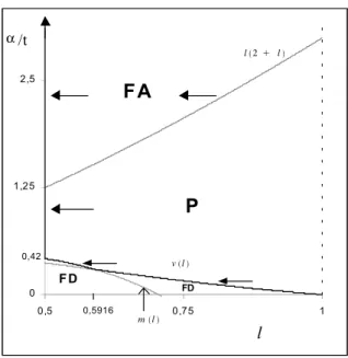
Observe in figure 1 that, for α < 3, the range ofe eα in which P occurs,
widens up and down as l rises. In other words, the more eastward the facility, the higher the probability that partial dispersion will emerge. The idea behind this is quite intuitive: whenever the public facility is sufficiently distant from the midpoint, it is also from firm A and price competition is
1 8
0 < DA(0,12) =125 −13α < 0.29e if 0.371 <α < 5/4. In any other case (F D or F A),e
DA(0,12) = 1/2. Note that the equilibrium price p∗A is continuous in the ratio α/t: the
lower the relative value of the public good, the lower the price charged by this firm (in order to secure a positive demand) as shown by (12). Forα ≥e 5
4, A prices at marginal
0 1,25 2,5 0,5 0,75 1
FA
P
v ( l ) v ( l ) v ( l ) v ( l ) α/t l F D l ( 2 + l ) l ( 2 + l )l ( 2 + l ) l ( 2 + l ) Figure 1: Equilibriasomewhat relaxed at the facility site. It follows, that firm B finds it profitable to locate at l in order to exploit the demand externality advantage.
Clearly, given α and t, firm B always prefers to observe a facility location decision which fosters the emergence of the partially-dispersed equilibrium since its profit in such a configuration is greater than the payoff under
max-imum differentiation 19; for the opposite reason, firm A strictly prefers a
symmetric maximum differentiation that yields the standard common pay-off t/2 (provided of course that the facility is not situated exactly at the east end):
ΠA(0, 1 − l) < t/2 < ΠB(0, 1 − l) (18)
Nevertheless, it is also easy to establish that δ
δtΠi(0, 1 − l) > 0 i = A, B (19)
for any 0 < α/t < l (2 + l) (partial dispersion). In other words, any policy re-ducing the transportation rate t will decrease respective profits under partial (full) dispersion. It follows that, even though firm B prefers configuration P for a given t, the two firms would, in fact, be better off in a city where trans-portations costs are very large, to such an extent that full dispersion would
1 9
Note that the payoff to firm B under partial dispersion is not necessarily maximized at l = 1 as shown in result 3 in appendix 9.7. Indeed, for 1 < α/t < 3, firm B prefers an interior facility location because the sum of the externality effect and the market area effect dominates the negative effect of price competition.
occur. Clearly, whichever the type of dispersion, the monopoly power gener-ated by geographical isolation increases with transportation costs incurred
by consumers, as often illustrated in the literature.20
Looking at the values of t and l which simultaneously maximize firm B’s profit, we have proved the following:
Result 2. Given α, the equilibrium profit of firm B is maximized whenever
t approaches ∞ and l = 1 (partial dispersion). The corresponding
equilibrium profit is ΠB(0, 0) ≈ 12t + 13α ; this firm captures
approxi-mately half of the market.21
In other words, whenever the facility is located at the east end of the city (l = 1) and t is very large, firm B’s profit exceeds the profit under F D (with
l < 1) by roughly 13α. A’s profit is lower than t/2 by the same amount.
On the contrary, A is better off when the public facility is centralized and α/t is very weak so as to make more likely the emergence of the fully-dispersed outcome.
Needless to say, the objective of the well-intentioned urban planner might be in discordance with the interests of firms. The former should also take into account the impact of changes in l (or t) on the surplus of consumers. This will be analyzed in sections 6 and 7. Yet, it is interesting to notice here that firms have strong incentives to lobby the city government, each duopolist trying to impose an opposite view on where should be situated the new facility–eastwards versus westwards–whereas they would agree on a weak transportation policy.
5
Optimality of equilibria
The objective of this section is to compare market outcomes derived earlier with the locations that a central planner would choose. In contrast to the standard welfare analysis of the Hotelling model, we cannot a priori assume that the socially-optimal locations will be symmetric. Indeed, the city plan-ner might consider the possibility of locating one firm at the facility site and the other one near the left border. This would induce a large share of the population to visit firm B (and thus the facility) while it would reduce transportation costs of those residing at the outskirts of the city. For a fixed
2 0Hotelling himself gave the intuition, p. 50:
”These particular merchants would do well, instead of organising improve-ment clubs and booster association to better the roads, to make transporta-tion as difficult as possible. (...) The objective of each is merely to attain something approaching a monopoly”
2 1Respective demands are easily obtained from (34) in appendix 9.4: D
A(0, 1) = 12−6tα ≈
facility location, the central city planner must select a pattern of locations among three possible configurations:
(1) either the two firms outside the facility location (dispersion)
(2) or, both at the place of the facility (full agglomeration or configuration F A)
(3) or, one firm at the facility location (say firm B) and its rival outside the facility location (partial dispersion).
We assume that firms are forced to price at marginal cost (standard,
see Tirole, 1988) and we denote bDA(a, b) ≡ DA(0, 0; a, b) the corresponding
quantity sold by firm A. One checks that the total welfare is equal to the aggregate surplus derived from the consumption of the public good (if any firm is at the facility site) minus the social transportation cost, which is given by: T (a, b) = Z DbA(a,b) 0 t(x − a) 2 dx + Z 1 b DA(a,b) t(1 − b − x)2 dx (20)
5.1
Dispersion
In the first configuration, the social transportation cost is identical to the one calculated in AGT since no one visits the facility. We know that the
socially-optimal pattern of locations is S = (14,14) (standard). This choice
of locations simply minimizes the total transportation cost which is equal
to T (14,14) = 481t. It is convenient for the remainder of the paper to define
WSY(a) as the total welfare in any symmetric configuration (a, a) (not only
S). The expression of WSY is given in the appendix (subsection 9.8.1) from
which we immediately derive the value of welfare in configuration S as:
WSY(1
4) = u−
1
48t (21)
5.2
Full agglomeration
In the second configuration, the whole population of consumers (normalized to 1) visits the facility site where it derives a constant utility α from the
provision of the public good. Using Di(l, 1 − l) = 12, one easily derives the
social transportation cost as in (45) (in appendix 9.8) and then calculates the total welfare under full agglomeration from (43) as:
WF A(l) = u + t · e α −1 3 + l(1 − l) ¸ (22)
5.3
Partial dispersion
Note that the assumption a < 1 − b = l might entail a loss of generality
(with the exception l = 12 which obviously restores symmetry). Indeed,
the city planner could consider to locate one firm at the facility place and its competitor on the right side in order to induce a larger share of the population to consume the public good or service. The welfare loss due to a larger amount of travel could, a priori, be counterbalanced by a higher surplus from the consumption of the public good. The two possibilities are analyzed in the two following subsections.
5.3.1 Firm A on the left of the facility site
Assume that the city planner first looks at the case a < l = 1 − b. Only
1 − bDA(a, l) proportion of the population visit the centrally-located firm B
and receive the benefit from the provision of the public good. Therefore, the total welfare is given by:
WP(a, 1 − l) = u + h 1 − bDA(a, 1 − l) i α − T (a, 1 − l) (23) where b DA(a, 1 − l) = 1 2(a + l) − e α 2 (l − a) = l2− a2− eα 2(l − a) (24)
after substituting pA= pB into (5).22 We next assume:
Condition 1 In any partially-dispersed configuration the city planner might
choose, the demand to A is positive: bDA(a, 1 − l) > 0 ⇔ α <e
l2− a2 ⇔ a <p(l2− eα)
In other words, the value of the public good must not be too high and/or the location chosen by the city planner should not be too close to the
facil-ity.23 In particular, we assumeα < le 2otherwise the whole population would
visit firm B at the facility location (whatever a may be); from the strict total welfare viewpoint, would be indifferent between the full agglomeration
situ-ation and the partially-dispersed equilibrium (a,12): the welfare is identical
in both cases and is equal to WP(1
2, 1
2). Indeed, in both configurations, the
whole population visits the facility site and derives the same net utility from the consumption of both goods, public and private, whatever the number of
2 2
Note that bDA is concave and reaches a global maximum atea = l −
√ e
α whereea = b
DA(ea, 1−l). Indeed, if firm A moves to the right then it looses some consumers in its close
hinterland because the travel cost to this firm rises while the net benefit from visiting B is unchanged. In other words, the facility location becomes relatively more attractive and the demand to A is strictly decreasing on the right ofea.
2 3Clearly, since prices are equal, there always exist some consumers situated between A
and B, possibly very close to the facility location, who patronize firm B. So necessarily, DB(a, 1 − l) > 0.
firms (one or two) at that location. The only difference is that under partial
dispersion, A does not produce any output. Put differently, forα > le 2, the
problem of choosing a location for firm A outside the facility location is sim-ply meaningless because this firm would not capture any positive demand. We thus suppose that, in such circumstances, the city planner prefers the fully-centralized outcome where firm A produces a positive output.
Before determining the welfare-maximizing firm A’s location, let us ana-lyze one important component of the total welfare. After some manipulation, one obtains the expression of the social transportation cost as in (46) (see appendix 9.8.3). For α = 0, the social transportation cost is minimized at
a = 13l. If the location of the facility (and thus firm B’s location) is fixed
at 34, we get the standard result of AGT: a = 14. If B is being imposed
the central location then we get a = 16 as transportation-cost-minimizing
location. This is not surprising since in the (no-facility) model of Hotelling
(with fixed prices), the socially-optimal locations of 3 firms is 16, 12, 56.
Of course, one can increase the second component of the welfare function by inducing a higher aggregate consumption of the public good–i.e., by
inducing more people to visit firm B. One shows that forα <e 49l2the demand
to A is increasing on [0,13l]. For α too high, more precisely fore 89l2 < αe
(< l2), one checks that bDA(a, 1 − l) = 0 at any a ≥ 13l. Hence, in these
two cases, the welfare-maximizing location will necessarily lie within the segment£0,13l£. For 49l2<α <e 8
9l2, it is a little bit more complex to predict,
at this stage, what will be the socially-optimal location of A because the
demand function has a positive value at 13l and exhibits a maximum on the
left of that location (see figure 2).24 We can however reasonably expect that,
again, the city planner will choose a location in the interior of [0,13l] because
a move eastwards translates into higher transportation costs.
We prove in the appendix that the unique value of a which maximizes the welfare function under partial dispersion, both locally and globally, is given by ba = 2 3l − 1 3 p l2+ 3αe (25)
with 0 <ba ≤ 13l as expected. One checks that condition 1 is satisfied near
ba, i.e., the demand facing A is positive (see appendix 9.9).25
2 4
Indeed, departing from1
3l, there exists two possible types of relocation that potentially
increases welfare (through a rise in the aggregate consumption of the public good, see figure 2): either near the left border, or within some segment [a1, a2]with a1>3l and a2
satisfying bDA(a2, 1 − l) = 0. 2 5As
e
α → 0, we have ba → 1
3l which re-establish consistently the transportation
cost-minimizing location (as indicated earlier). Notice also that the demand to A is at most 2 3
whenever the public facility is located at the east end of the line andα → 0 (firm A beinge optimally-located at 13).
0 0.05 0.1 0.15 0.2 0.25 0.3 0.1 0.2 0.3 a0.4 0.5 0.6 0.7 Figure 2: Demand to A ( l = 1 − b = 0.75)
5.3.2 Firm A at the facility site
We show in the appendix that any configuration involving a = l < 1 − b is suboptimal from the welfare viewpoint. We first determine the
socially-optimal location b = bb subject to a = l < 1 − b ≤ 1 and then we show that
the corresponding value of the welfare is lower than WP(ba, 1 − l) calculated
in the preceding section. We conclude that in any asymmetric pattern of
locations involving B at l > 12, the omniscient central planner would locate
A at ba < l as defined in (25) above. We shall speak of optimal partial
dispersion or configuration OP = (ba, 1 − l).
5.4
Optimal pattern of locations
Proposition 3 Assume that the public facility is located somewhere in the
second half-segment.
• For a very low eα, the optimal locations are given by the (standard)
transportation-cost-minimizing solution: e
α < y(l) ⇒ (ba,bb) = S = (1/4, 1/4)
• On the other hand, if the relative value of the public good is very high then the socially-optimal pattern of locations exhibits both firms at the facility site:
e
α ≥ l2 ⇒ (ba,bb) = F A = (l, 1 − l)
• For intermediate values of the relative transportation cost parameter, the city planner finds a compromise between saving on transportation costs and inducing a high proportion of the population to consume the
public good ; s/he locates one firm at the facility place and its rival at a more suburban interior site:
(ba,bb) = OP = (2 3l − 1 3 p l2+ 3α, 1 − l)e
• When it emerges as a market outcome, full agglomeration is socially-optimal.
• Under laissez-faire, any dispersion, partial or full, is excessive: when the market outcome is P = (0, 1 − l) it should be F A or OP (or even S whenever l is close to the east end and α near 0). When dispersion is maximal, the city planner would prefer it partial with one firm at
the facility site, or S = (1/4, 1/4) for a very weak α (or even F Ae
whenever l is close to the midpoint and 0.25 ≤ l2<eα < 0.371).26
Proof. In the appendix.
In some circumstances, firm B optimally locates at the facility–a move which certainly fosters the consumption of the public service–but its rival
is still suboptimally located at the outskirts. For a low eα < y(l) and l
approaching 0.75, it becomes more and more interesting to induce OP 6= S with firm B at the facility site, in order to exploit the externality. Indeed, when l is close to 0.75, OP retains a high proportion of the social benefits of the configuration S = (1/4, 1/4) while adding the aggregate surplus derived
from the consumption of the public good.27
0 1,25 0,5 0,75 1 FA P α αα α/t l FD
FA
OP
OP
0,25 S S llll2222 0 0,25 0,5 0,75 1 FA α αα α/t l OP OP S S y ( l ) y ( l ) y ( l ) y ( l ) llll2222 FD P 2 6In one particular situation, the partially-dispersed market outcome is ”nearly” socially-optimal: ifeα ≈ l2 and P emerges, then
ba ≈ 0 = a∗ (i.e., OP ≈ P ). 2 7
Observe in the figure above that for a given l = 0.75 = 1 − b and α = 0 (OP ), the area S consistently vanishes.
6
Optimal location of the facility
We have already discussed the effects of a change in l on the spatial structure of the business sector. Here, we tackle the problem of the optimal location of the public facility from the welfare viewpoint. We suppose that the choice of l is made in a stage prior to the non cooperative location-then-price game. This allows us to look at business relocation effects which are not calculated
in the standard cost-benefit analysis of the building of a new facility.28 Since
α is constant, we can neglect the cost of providing of the public service, mainly the fixed cost of building the facility. Indeed, this cost only shifts the welfare functions without changing the results below. The total welfare is thus again equal to the total surplus derived from the aggregate consumption of the private good (plus the consumption of the public good, should some firm(s) be located at l) minus the social transportation cost. The latter
component is given by (20) where bDAis replaced by the demand to A under
laissez-faire: DA(a∗, b∗) = DA(0, 0) = 12 ifeα < v(l) DA(0, 1 − l) = l(2+l)−e6l α if v(l) <α < l (2 + l)e 1 2 ifα > l (2 + l)e (26)
from propositions 1 and equation (34) in the appendix. When the market outcome is fully-agglomerated, firms price at marginal cost and the expres-sions of respective demands and welfare are the same as in the preceding section (where firms were forced to set prices to zero). One easily checks that the transportation cost function (45) is minimized when the city plan-ner centralizes the public facility. Hence, the value of the social surplus is immediately obtained from (22):
WF A(1
2) = u + α −
t
12 (27)
Now, in the fully-dispersed subgame perfect outcome, the social transporta-tion cost functransporta-tion and the total welfare functransporta-tion have been established again
in the preceding section. Indeed, by symmetry, DA(a, b) = bDA(a, b) = 12
whenever a = b 6= 1 − l. Moreover, the value of the social transportation
cost is equal to 12t , i.e., the value calculated under full agglomeration above.
Indeed, in both configurations F A and F D, the first half of the population
patronizes firm A which is situated at one end of the half-segment (at 12 or
at 0). The only difference is that, under F D, no one consumes the public good. Thus, we deduce the welfare under full dispersion from (27) as
WSY(0) = u − t
12 (28)
2 8
see also, in different contexts, Combes and Linnemer (2000), p. 16 and Thisse and Wildasin (1992).
If the city planner aims to induce such a pattern of firms’ locations, s/he
must simply locate the facility at any l satisfyingα < v(l).e
Now, in the eyes of the city planner, each one of the configurations F A and F D ”solely” competes with partial dispersion (see figure 1). Indeed, the latter configuration leads to a more balanced pattern of shopping trips while retaining a high social benefit for those who both shop at B and consume the public good (recall proposition 3). As opposed to the two pre-ceding configurations, in the partially-dispersed (laissez faire) equilibrium,
the transportation cost functions and the total welfare–denoted WP
∗ , are
different from the ones established in the optimality analysis.29 Indeed,
the overall urban system is now affected by non cooperative price decisions through changes in respective equilibrium demands. We now state the main proposition of this section:
Proposition 4 Given α and t, the unique socially-optimal location of the
facility is bl= 0.5916 ≤ v−1(α/t) < 1 1 2 < m−1(α/t) < 0.5916 1 2 if 0 < α/t < 0.291 if 0.291 < α/t < 0.42 α/t > 0.42
The market outcome is partially-dispersed, except for α > 1.25 wheree
firms are induced to agglomerate at the facility central site.
Proof. In the appendix.
In the following figure, the optimal location of the facility is depicted by the bold line and the arrows indicate increases in the total welfare under
partial dispersion or full agglomeration.30 Observe that the city planner
necessarily decides to induce some positive consumption of the public service (F D is dismissed). The curve m(l) plots the first order condition for an interior maximum (the second-order condition being met). In fact, for 0 < e
α < 0.291, in order to avoid the emergence of F D, the city planner should place the facility (obviously in the P area) almost on v(l), that is, at some
location v−1(eα) + ², where ² > 0 is arbitrarily small.31 In the competitive
fully-agglomerated outcome, firms do not earn any (supranormal) profits at the central site. This pattern of locations maximizes the consumer’s surplus
which is equal to: WF A(12) = u + α − 12t. Clearly, the higher α (and the
lower t), the higher consumer welfare in the fully agglomerated outcome. 2 9see equations (53) and (54) in the appendix.
3 0
Recall here that P stands for partial dispersion under laissez-faire and should not be confused with the optimal dispersion OP analyzed before.
3 1
Example: for α = . 160 576 211 t, let ² = 0.0001 and locate the facility at v−1(α/t)+² = 0.750001so that the profit under P is equal to 0.500 000 029t > t/2, that is just enough to dismiss F D.
0 1,25 2,5 0,5 0,75 1
FA
P
v (l ) α/t l 0,5916 0,42 m (l ) F D FD l (2 + l )Figure 3: Optimal facility location
7
Policies aiming at a decrease in
t
Once the public facility has been built at some location l, the city planner can still affect significantly the urban structure by modifying the quality of the transportation system (which determines the rate t). Many improvements of the urban transportation networks can be achieved in short run: comfort, safety, frequency of service (for public mass transit). The city planner might also add new lines or increase the number of buses, for example. As also suggested by Thisse and Wildasin (1992), p. 102:
”Some tax policies, such as gasoline taxes, can also affect travel costs. (...) as do highway and bridge tolls and the pricing of public trans-portation”.
For fixed firms’ locations, a reduction in t clearly improves the total wel-fare. Nevertheless, this is misleading since firms may relocate. In particular, as argued before, the city planner could prefer to foster some dispersion in order to get a more balanced system of households trips. Yet, we proved the following intuitive non-trivial result:
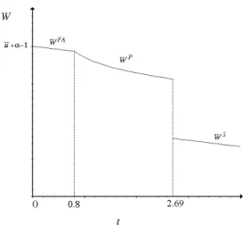
Proposition 5 Whatever the value of the public good and the location of the
facility, the total welfare is globally-maximized at t = 0 (full agglomeration). Finally, as argued before, it is easier to change the transportation cost parameter once the public facility has been built than to do the reverse.
Figure 4: Impact of t on welfare
Therefore, it is natural to suppose that the choice of l is prior to any trans-portation policy decision and, from propositions 4 and 5, we conclude:
Proposition 6 Assume that t ∈]0, ∞[. From the welfare viewpoint, it is
optimal to centralize the provision of the public service (l = 1/2) and then
to reduce the transportation cost near zero.32
8
Conclusion
The clustering of firms selling a similar product or service is often observed in real urban life. Our paper has explored one possible explanation to this phenomenon, namely the fact that a public facility may serve as agglomer-ation point, as already suggested by Thisse and Wildasin (1992). We have added this centripetal force to the standard spatial setting, assuming that people have a preference for ”one-stop” multipurpose trips to the facility site. Minimum differentiation at the facility place–what we have called full agglomeration–may indeed emerge as an efficient market outcome, without relaxation of price competition. The second part of this result may surprise at first glance since it is opposed to the argument generally put forward in the literature–which precisely stresses on the need of relaxing price compe-tition somehow or other. Yet, the idea is very simple: for low transportation costs compared to the value of the public service, the facility location is a
3 2
Proof. Indeed, WAreaches a maximum values of u + α at t = 0, wherever the facility may be. Thus, the choice of l is relevant only if t > 0. For t ' 0, the backwards-induction (optimal) facility location is l = 1/2.
dominant strategy, and de facto the only place that guarantees a positive market share.
Another striking result is the fact that for a wide range of the ratio transportation cost/value of the public service, asymmetric equilibria emerge even if the public facility, when built at the midpoint, balances perfectly the demand between the two half-segments. In these equilibria, only one oligopolistic firm locates at the facility place in order to exploit the ex-ternality advantage. Yet, any dispersion, partial or full, is excessive from the city planner viewpoint–even though, in some circumstances, one firm optimally locates at the facility.
Finally, we have stressed the role of the city planner in shaping the business spatial structure. In particular, we have established the non-trivial result that the lower the transportation cost, the higher the total welfare. If the city planner is able to lower transportation costs ”near zero”, then it is optimal to locate the facility at the midpoint. On the other hand, if there exists some impediments to the reduction of urban transportation costs, then the city planner would be well-advised to locate the facility at a more eastern site. Indeed, such a configuration results in a more balanced pattern of households trips while retaining some welfare benefits from the provision of the public service to a large share of the population.
Of course, the results of our paper must not be viewed as a guide to real policy. However, our analysis has confirmed that any cost-benefit analysis of the building of a new public facility, or any evaluation of transportation policy (which is sensitive to the facility location), should take into account the impact on strategic locational choices made by oligopolists (see also Thisse and Wildasin, 1992, 1995).
One limitation of our model is the fact that multipurpose shopping is not reasonable for some public facilities such as hospitals or schools; as emphasized by Thisse and Wildasin (1995), p. 408: ”you do not buy shoes on the way to the hospital”. We hope to modify the present framework in order to incorporate independent trips for this type of facility. We expect the establishment of the existence of equilibrium in prices to be non-trivial. Future research is also needed in order to determine the socially-optimal level of provision of public service (i.e., optimal facility size or quality). One should distinguish between pure and congested local public goods. Con-gestion at the site level could make the emergence of a partially-dispersed outcome more desirable than agglomeration. Also, it would be interesting to incorporate two or three major transportation nodes, as well as two or three competing juridictions for some types of facility such libraries.
9
Appendix
9.1
Proof of result 1
One readily checks from equation (5) that if t
α >
1
(l − a) (2 + l + a) (29)
then A is in position to attract some consumers by setting a price pA =
PA(pB) (possibly very small) as expressed in (9). On the other hand, if the
last inequality is not satisfied then firm B optimally monopolizes the whole market by setting a price
p◦B(pA) = pA+ α − t(l + a)(l − a) (30)
such that DA= 0.33 In such an event, one verifies that the mirror game in
prices converges to pA= 0, p
◦
B(0). If (29) does not hold that the equilibrium
prices is simply the solution of (9)-(10) as expressed in (12)-(13). Q.E.D.
9.2
Proof of lemma 3
By contradiction, assume thatea and 1 − eb 6= l is an equilibrium of the first
stage. From AGT, ea = eb = 0 necessarily and respective maximum profits
are equal to 2t = pi
2 (i = A, B, see AGT). On the other hand, by virtue of
lemma 1, the payoff to B after relocation at l is:
p◦B(0) = α − tl2 (31)
We have:
p◦B(0) > 2t ⇔ α − tl2 = t(α − le 2) > 2t ⇔ α >e 12 + l2
which is clearly satisfied for any eα > l (2 + l) and establishes a
contra-diction. Q.E.D.
9.3
Proof of proposition 1
Assume first a < l. Let us show that ΠB(a, 1 − l) > t/2 ≥ ΠB(a, b). Since
ΠB(a, 1 − l) = p◦B(0) = α − t(l + a)(l − a) is increasing with a it suffices to
establish that α/t − l2 > 1/2. This has been done in the proof of lemma 3
(Q.E.D). 3 3
Assume that (29) does not hold. Then, for fixed locations and a fixed price pA, the
one-variable profit function ΠB(pA,.) is continuous on [0, ∞[ : it is the 45oline on
h
0, p◦B(pA)
i and it is strictly concave, decreasing onhp◦B(pA), Π−1B (0)
h . We have: ΠB(pA,.) = p ◦ B(pA) > PB(pA), that is, p ◦ B(pA)is a global maximum of ΠB(pA,.).
Second, assume a > l = 1−b and eα ≥ (3−l) (1 − l). Firm B monopolizes the market (exchange A with B, and a with 1 − b in lemma 2) and optimally
sets the following price: peB(0, a) ≡
defα−t(a−l)(2−l−a). Let us prove again
that it is greater than the maximum profit under full dispersion: epB(0, a) >
t/2 ? One checks that (i) peB is decreasing with a and (ii) peB(0, l) = α >
t/2 so that, necessarily,peB(0, a) > t/2 ≥ ΠB(a, b) for all a > l.
Finally, if a = l then clearly ΠB(l, 1−l) = 0 = ΠB(l, b) where b 6= 1−l.
To sum up: ΠB(a, 1 − l) ≥ ΠB(a, b) for all b ∈ [0, 1], that is, b = 1 − l
is a weakly dominant strategy for firm B. By symmetry, a = l is a weakly
dominating strategy for firm A. Q.E.D.
9.4
Proof of lemma 4
Let us show that firm A can always find a location close to the west end–
i.e., in some interval [0, s(α, l)[, such that it attracts a positive demand ine
any equilibrium of the last stage. Such a segment of potential locations for
A must satisfy (29), that is: (l − a)(2 + l + a) > eα. The relevant root of the
second-degree equation in the last inequality is:
a = −1 +p(1 + l)2− eα ≡
defs(α, l)e (32)
One easily checks that: (i) (1 + l)2− eα > 0, (ii) s(α, l) is decreasing withe αe
and (iii) 0 ≤ s(eα, l) < l.34 Thus, A is always in position to find a location
near the left border where it captures a positive demand after solving for price competition. (Q.E.D).
Now let us find the optimal location a∗ ∈ [0, s(eα)[. Firstly, for fixed
locations, the equilibrium price set by firm A is as follows:
pA(a, 1 − l) =
α 3 £
et(l − a) (2 + a + l) − 1¤ (33)
after using result 1; the demand to A is given by:
DA(a, 1 − l) = pA(a, l) 2t(1 − l − a) = £ et(l − a) (2 + a + l) − 1¤ 6et(l − a) (34)
after substitution of b = 1 − l. From the two last expressions, one easily computes the reduced-form profit function of firm A. However, it is easier to analyze the sign of the partial derivative with respect to a as follows:
δ δa(pADA) = pA 2t(l − a) · 2δpA δa + pA (l − a) ¸ (35)
Indeed, the demand to A, and consequently pA, is necessarily positive in
any outcome of the last stage and it suffices to analyze the sign of the 3 4
bracketed term, that we denote G(a). One calculates δpA
δa = − 2
3t (1 + a) <
0, and substituting this and Eq.(33) into Eq.(35), one obtains after some manipulations: G(a) = 13 h t (l − 2 − 3a) − l−aα i < 0
(since a < l < 1). This achieves the proof of lemma 4. Q.E.D.
9.5
Exclusion of the case
l
≤ a ≤ 1 − b ≤ 1
Assume l ≤ a < 1 − b ≤ 1. From AGT, the optimal location of firm A is a∗ = l.
• Case #1: (3 − l) (1 − l) < eα < l (2 + l)
From lemma 2, the demand to firm B is equal to zero for all b ∈ ]0, 1 − l] . However, firm B can increase its profit by relocating at the left end of the city, playing the role of firm A in proposition 2. (Q.E.D).
• Case #2: eα < (3 − l) (1 − l)
In any outcome, the demand to firm B must be positive since otherwise it would be incited to relocate at the left end of the city. We know that firm B can indeed always find a location close to the right end such that
DB(l, b) > 0 is satisfied.35 Firm A benefits from the best environment:
∆f (a, b) = −α. Substituting this into equations, we derive the unique Nash equilibrium in prices as:
p∗
A(l, b) = t(1 − b − l)(1 +l−b3 ) +
α 3
p∗B(l, b) = t(1 − b − l)(1 +b−l3 ) +−α3
After substitution into (5), we get the demand facing firm B as a unique function of locations: DB(l, b) = 1 6 t (1 − b − l) (b + 3 − l) − α t (1 − b − l) (36)
The value of the profit to firm B is as follows: ΠB(l, b) = 181 (t(1−b−l)(b+3−l)−α)
2
t(1−b−l)
and we also get
dΠB db (l, b) = 1 18(t (1 − b − l) (b + 3 − l) − α) −t(1−b−l)(3b+l+1)−α t(−1+b+l)2 3 5
Since DB(l, b) > 0 by assumption, observe that
t (1 − b − l) (b + 3 − l) − α > 0
necessarily. Hence, dΠB
db (l, b) < 0 ⇒ b∗ = 0. The value of the profit is
immediately obtained as being:
ΠB(l, 0) = [t (1 − l) (3 − l) − α]
2
18t (1 − l) (37)
The payoff to firm A is higher than ΠB(l, 0) and is given by:
ΠA(l, 0) = [t (1 − l) (3 + l) + α]
2
18t(1 − l) (38)
Next, consider a relocation of B at the west end of the city (b = 1) and solve for price competition. The reduced-form payoff function of a firm situated at the left end while its competitor is at the facility location is given by (16):
ΠB(l, 1) = [tl (2 + l) − α]
2
18tl (39)
Hence, we derive the following ratio of payoffs to B:
ΠB(l,1) ΠB(l,0) = (l(2+l)−eα)2 ((1−l)(3−l)−eα)2 (1−l) l
Let us prove that it is greater than unity. Observe that (1−l)l < 1 for
l > 12. We can however rewrite the above ratio as follows:
h l(2+l)−eα (1−l)(3−l)−eα(1−l)l i2 l 1−l
Clearly, it would suffice to show that the bracketed term is greater than 1: l(2+l)−eα (1−l)(3−l)−eα (1−l) l > 1 ⇔ (2 + l) −e α l > (3 − l) − e α 1−l ⇔ (2 + l) +1−leα > (3 − l) + eαl ⇔ (2 + l) > (3 − l) + eα(1l −1−l1 ) ⇔ (2 + l) > (3 − l) + eαl(1−l)1−2l
which is necessarily checked for l > 12. Thus ΠB(l, 1) > ΠB(l, 0): B
is incited to relocate at the west end (Q.E.D). For l = 12, B is indifferent
between either ends of the line. This achieves the proof that 12 < l ≤ a ≤
9.6
Proof of proposition 2
9.6.1 Lemma 4.1.
Assume a = 0 and l 6= 1. There exists a threshold value et0 such that et >
et0 ⇒ ΠB(0, 1 − l) < 2t: B locates at the east end (b = 0).
Proof. Assume l 6= 1. Since, the endpoint dominates any location
outside the midpoint, it suffices to compare equation (17) with the profit
under maximum differentiation (AGT), that is, ΠB(0, 0) = 2t :
(t 3l(4−l)+ 1 3α) 2 2tl < t 2 ⇔ ³ et 3l (4 − l) + 1 3 ´2 − et2l < 0
The relevant root of the polynomial in the last inequality is et0=
l2− 4l − 3√l
l (l − 1) (l2− 7l + 9) (40)
(the second root is negative). Define also v(l) = 1/et0 the corresponding
threshold value ofeα. Since the above polynomial is concave in et, we deduce
that for any et >et0 (⇔ eα < v(l)), ΠB(0, 1 − l) < t2. If l = 1, then b = 0 is
clearly a dominant strategy for firm B.
9.6.2 proof of (ii)
Assume v(l) <α < l (2 + l) and l 6= 1. First, we have proved that Πe B(0, 1 −
l) > 2t ≥ ΠB(0, b), ∀b 6= 1 − l. Thus b∗= 1 − l maximizes ΠB(0, .) on [0, 1].
Second, assume that b∗ = 1 − l is fixed. By lemma 4, a∗ = 0 maximizes
ΠA(., 1 − l) on [0, l[. Moreover, A is worse off on the right side of (or at) the
facility location, as established in subsection 9.5 (reverse the role of A and B). Thus, (0, 1 − l) is a pure strategy Nash equilibrium in locations. It is unique since a = l < 1 − b cannot be an equilibrium. (Q.E.D).
9.6.3 proof of (i)
Let 0 < α < v(l) and assume be ∗ = 0. From AGT, δaδΠA(a, 0) < 0: the
optimal location of A on [0, l[ is a = 0. For the same reason, the optimal location of A on [l, 1] is a = l. One easily checks that v(l) < (3 − l)(1 −
l),36 which implies that the demand to B is positive after solving for price
competition (see subsection 9.5, case #2 above). The payoff to A is ΠA(l, 0)
as given by Eq. (38). Let us show thatα < v(l) ⇒ Πe A(l, 0) < 2t. One first
obtains the following implication:
t 2 − ΠA(l, 0) > 0 ⇔ α < 2l + le 2 − 3 + 3p(−l + 1) = defz(l) 3 6 Indeed, (3 − l)(1 − l) − v(l) = 3 (1 − l) l+ √ l(3−l) l(4−l)+3√l> 0.