DESY 17-096
Enabling rootless Linux Containers in multi-user
environments: the udocker tool
Jorge Gomes1, Emanuele Bagnaschi2, Isabel Campos3,
Mario David1, Lu´ıs Alves1, Jo˜ao Martins1, Jo˜ao Pina1, Alvaro L´opez-Garc´ıa3, and Pablo Orviz3
1
Laborat´orio de Instrumenta¸c˜ao e F´ısica Experimental de Part´ıculas (LIP), Lisboa, Portugal
2Deutsches Elektronen-Synchrotron (DESY), 22607 Hamburg, Germany 3
IFCA, Consejo Superior de Investigaciones Cient´ıficas-CSIC, Santander, Spain
June 5, 2018
Abstract
Containers are increasingly used as means to distribute and run Linux services and applications. In this paper we describe the architectural design and implementation of udocker, a tool which enables the user to execute Linux containers in user mode. We also present a few practical applications, using a range of scientific codes characterized by different requirements: from single core execution to MPI parallel execution and execution on GPGPUs.
1
Introduction
Technologies based on Linux containers have become very popular among soft-ware developers and system administrators. The main reason behind this suc-cess is the flexibility and efficiency that containers offer when it comes to pack-ing, deploying and running software.
A given software can be containerized together with all its dependencies in such a way that it can be seamlessly executed regardless of the Linux distribution used by the designated host systems. This is achieved by using advanced features of modern Linux kernels [1], namely control groups and namespaces isolation [2, 3]. Using both features, a set of processes can be placed in a fully isolated environment (using namespaces isolation), with a given amount of resources, such as CPU or RAM, allocated to it (using control groups). We call “container” this encapsulated group of processes.
Containers do not need to boot an operating system kernel, instead they share the one of the host system. Therefore they can be seen as a lightweight approach to virtualization, when compared with conventional Virtual Machines
(VM) such as the ones provided using para-virtualization or hardware virtual machines.
As a consequence, a given physical system may host many more containers than virtual machines, as the first ones use less hardware resources (notably memory). Moreover, transferring, starting and shutting down containers is usu-ally much faster than performing the same operations on a conventional virtual machine.
The idea of operating-system-level virtualization is not new. The origin can be traced back to the chroot system call (introduced in 1979), which enables changing the root directory for a given process and its children. The concept was further extended with the introduction of the jailed systems of BSD [4] (released in 1998). However the developments required at the level of the Linux kernel to have a consistent and robust implementation have taken a few years more to crystallize. The Control groups technology, also known as cgroups, is present in the Linux kernels since version 2.6.24 (released in 2008). Support for namespaces was first introduced in the Linux kernel 2.4.19 (released in 2002), with additional namespaces and enhancements being added since. However it was only with the introduction of Docker [5] that containers gained widespread adoption in Linux.
Docker simplifies the creation, distribution and execution of Linux contain-ers. Besides providing the tools to build containers and execute them, it also supports container repositories (such as the Dockerhub [6]), enabling the upload and the download of container images.
Docker container images make use of a layered filesystem where changes are added as new layers. Using this approach, a new Docker image can be created from an existing one simply by reusing and sharing its layers. Sharing layers among images saves storage space and minimizes downloads.
Because of these very appealing features described above, Docker is now widely used to containerize both services and applications. However Docker presents limitations especially when it comes to deploy containers in multi-user systems. In Docker, processes within the container are normally executed with root privileges under the Docker daemon process tree, thus escaping to resource usage policies, accounting controls, and process controls that are imposed to normal users. In addition, users authorized to access the Docker remote API can easily gain privileged access to the host system. Due to these limitations Docker is not generally available in multi-user systems.
Unfortunately most scientific computing resources such as High Performance Computing (HPC) systems, Linux clusters or grid infrastructures are multi-user systems. Therefore the adoption of Docker in these infrastructures has been very restricted.
Another limitation of Docker concerns the support for parallel applications that require network communication across multiple hosts. For security reasons Docker uses network namespaces, making direct communication between con-tainers across different hosts more difficult with respect to normal processes. The use of network namespaces can be disabled but, opting for this solution, results in a system security issue, as privileged processes running within the
container may interfere with the host network stack. Access to host devices from within the container is similarly problematic for the same reasons.
The Docker layered filesystem has many advantages but it is also slower than accessing the host filesystem directly. Furthermore files in existing layers cannot be deleted or changed, instead they are hidden or overridden by an upper layer. Consequently container images grow in size when modified and the only way to keep their size at acceptable level is to rebuild them from scratch.
The applicability of Docker to scientific computing has been hampered by the limitations we have highlighted in the prevision paragraphs. As a consequence, alternative solutions such as Singularity [7] or Shifter [8] have been developed. However these solutions also have their own limitations. They generally require administrator privileges both for installation and execution, or alternatively require recent Linux kernel features such as unprivileged namespaces which are still not widely available in scientific computing systems.
In this work we address the problematic of executing Docker containers in user space, i.e. without installing additional system software, without requiring any administrative privileges and in a way that respects resource usage policies, accounting and process controls. Our aim is to empower users to execute appli-cations encapsulated in Docker containers easily in any Linux system including computing clusters without system administrator intervention and regardless of Docker being locally available.
In section 2 we will describe the architectural elements of the tool we have developed to address the above mentioned problems and shortfalls. The re-maining of the paper is devoted to describe the practical applicability of this middleware. We describe how our solution can be applied to three very different use cases which we believe are representative of the current scientific-computing landscape.
The first use case describes an application highly complex due to the inter-play of library dependencies, legacy code, library and software requirements. The second case addresses the usage of containers in MPI parallel applications using Infiniband and/or TCP/IP. Finally we also show how to target specialized hardware accelerators such as GPGPUs.
All the tools presented here are open-source and may be downloaded from our public repository [9].
2
Architectural design
To overcome the limitations mentioned in section 1 we have explored the possi-bilities available to run applications encapsulated in Docker containers in user space in a portable way. Our technical analysis is as follows.
2.1
Technical Analysis
Most scientific applications do not require the full set of Docker features. These applications are usually developed to be executed in multi-user shared
environ-ments by unprivileged users. Therefore features such as isolation are not strictly needed as long as the applications are executed without privileges. The funda-mental features that make Docker appealing as a means to execute scientific applications are thus the following:
• the ability to provide a separate directory tree where the application with all its dependencies can execute independently from the target host; • possibility of mounting host directories inside the container directory tree,
which is convenient for data access; • easy software packaging with Dockerfiles; • reuse of previously created images;
• easy sharing and distribution of images via Docker repositories such as Docker Hub and many others;
• simple command line and REST interfaces.
Several of these features such as creating containers and pushing them into repositories can be accomplished from the user desktop or portable computer using Docker directly. Therefore we assume that Docker can be used to prepare the containers and that the focus should rather be put on enabling the execution of the created containers in systems where Docker is unavailable.
The most complex aspect is to provide a chroot-like functionality so that Docker containers can be executed without conflicting with the host operating system environment. The chroot system call requires privileges and therefore would collide with our objective of having a tool that would not require privileges or installation by the system administrator. Three alternative approaches to implement chroot-like functionality without privileges were identified:
• use unprivileged User Namespaces;
• use PTRACE to intercept calls that handle pathnames; • use LD PRELOAD to intercept calls that handle pathnames.
The use of unprivileged User Namespaces allows a non-privileged user to take advantage of the Linux namespaces mechanism. This approach is only usable since kernel 3.19. Unfortunately the implementation of unprivileged User Namespaces exposes the processes running inside the container to limitations especially in terms of mappings of group identifiers. Furthermore this approach does not work on certain distributions such as CentOS 6 and CentOS 7, which do not provide kernels having the necessary features. Due to these limitations this approach was initially discarded.
The PTRACE mechanism enables tracing of system calls making possible to change their calling parameters in run time. System calls that use pathnames can be traced and dynamically changed so that references to pathnames within
the container can be dynamically expanded into host pathnames prior to the system calls and upon their return. The biggest drawback of using PTRACE to implement chroot-like functionality is the impact on performance. An external process needs to trace the execution of the application, stop it before each system call, change its parameters when they reference pathnames, and continue from the same point. If the system call returns pathnames a second stop must be performed when the call returns to perform the required changes. In older kernels (such as in CentOS 6) all system calls need to be traced. In more recent kernels is possible to use PTRACE with SECCOMP filtering to perform selective system call tracing thus allowing to restrict interception only to the set of calls that manipulate pathnames. The impact of using PTRACE depends on the availability of SECCOMP and on how frequently the application invokes system calls.
The LD PRELOAD mechanism allows overriding of shared libraries. In practice this approach allows to call wrapping functions where the pathnames can be changed before and after invoking the actual system functions. The LD PRELOAD mechanism is implemented by the dynamic loader ld.so. The dynamic loader is an executable that finds and loads shared libraries and pre-pares programs for execution. The dynamic loader also provides a set of calls that enable applications to load further dynamic libraries in run time. When a shared library pathname does not contain a slash the dynamic loader searches for the library in the directory locations provided by:
• DT RPATH dynamic section attribute of the ELF executable; • LD LIBRARY PATH environment variable;
• DT RUNPATH dynamic section attribute of the ELF executable; • cache file /etc/ld.so.cache;
• default paths such as /lib64, /usr/lib64, /lib, /usr/lib.
Due to this behavior, libraries from the host system may end-up being loaded instead of the libraries within the chroot-environment. Furthermore the follow-ing limitations apply:
• this approach depends on dynamic linking and does not work with stati-cally linked executables;
• the absolute pathname to the dynamic loader is encoded in the executa-bles, leading to the invocation of the host dynamic loader instead of the dynamic loader provided in the container;
• dynamic executables and shared libraries may also reference other shared libraries, if they have absolute pathnames then they may be loaded from locations outside of the container.
2.2
The udocker tool
To validate the concept we developed a tool called udocker that combines the pulling, extraction and execution of Docker containers without privileges. udocker is an integration tool that incorporates several execution methods giv-ing the user the best possible options to execute their containers accordgiv-ing to the target host capabilities. udocker is written in Python and aims to be portable. udocker has eight main blocks:
• user command line interface; • self installation;
• interface with Docker Hub repositories; • local repository of images;
• creation of containers from images; • local repository of containers; • containers execution;
• specific execution methods.
udocker provides a command line interface similar to Docker and provides a subset of its commands aimed at searching, pulling and executing containers in a Docker like manner.
The self installation allows a user to transfer the udocker Python script and upon the first invocation pull any additional required tools and libraries which are then stored in the user directory. This allows udocker to be easily deployed and upgraded by the user himself. udocker can also be installed from a previously downloaded tarball.
The Docker images are composed of filesystem layers. Each layer has meta-data and a directory tree that must be stacked by the layered filesystem to obtain the complete image. The Docker layered filesystem is based on UnionFS [10]. In UnionFS file deletion is implemented by signaling the hiding of files in the lower layers via additional files that act as markers white-outs. We therefore implemented the pulling of images by downloading the corresponding layers and metadata using the Docker Hub REST API. A simple repository has been im-plemented where layers and metadata are stored. Layers are shared across the images to save space. The repository is by default placed in the user home di-rectory. To prepare a container directory tree, the several layers are sequentially extracted over the previous ones respecting the white-outs. File protections are then adjusted so that the user can access all container files and directories. The container directory tree is also stored in the local repository. The container execution is achieved with a chroot-like operation using the previously prepared container directory tree.
udocker implements the parsing of Docker container metadata and supports a subset of metadata options namely: the command to be invoked when the container is started, mount of host directories, setting of environment variables, and the initial working directory.
The PTRACE execution method was implemented using PRoot [11], a tool that provides chroot-like functionality using PTRACE. PRoot also provides mapping of host files and directories into the container enabling access from the container to host locations. We had to develop fixes for PROOT to make SECCOMP filtering work together with PTRACE due to changes introduced in the Linux kernel 3.8 and above. A fix for proper clean-up of temporary files was also added.
The LD PRELOAD method is based on Fakechroot [12] a library that pro-vides chroot-like functionality using this mechanism, and is commonly used in Debian to install a base system in a subdirectory. Fakechroot provides most of the wrapping functions that are needed. However due to the previously de-scribed behavior of the dynamic loader, applications running under Fakechroot may unwillingly load shared libraries from the host. udocker implements several strategies to address these shortcomings.
• Replacement of the dynamic loader pathname in the executables header, thus forcing the execution of the loader provided with the container. • Replacement of DT RPATH and DT RUNPATH in the executables,
forc-ing the search paths to container locations.
• Replacement of shared library names within the headers of executables and libraries, forcing them to container locations.
• Extraction of shared libraries pathnames from ld.so.cache which are then modified and added to LD LIBRARY PATH.
• Interception of changes to LD LIBRARY PATH forcing the paths to con-tainer locations.
• Prevent the dynamic loader from accessing the host ld.so.cache
• Prevent the dynamic loader from loading libraries from the host /lib64, /usr/lib64, /lib, /usr/lib.
Changes to executables and libraries are performed using PatchELF [13]. PatchELF was enhanced to manage the pathname prefixes of: the dynamic loader within executables, library dependencies and their paths in executables and shared libraries. The ld.so executable within the container can also be modified by udocker to prevent the loading of shared libraries from the host. All the above changes are performed automatically by udocker depending on the execution mode selected. The Fakechroot library was heavily modified to address multiple limitations, change executables and libraries in run time, and to provide better mapping of host directories and files inside the container.
The support for unprivileged User Namespaces and rootless containers was implemented using runC [14], a tool for spawning and running containers accord-ing to the Open Containers Initiative OCI [15] specification. udocker translates Docker metadata and the command line arguments to build a matching OCI configuration spec that enables the container execution in unprivileged mode.
All external tools including PRoot, PatchELF, runC and Fakechroot are provided together with udocker. The binary executables are statically com-piled to be used across multiple Linux distributions unchanged and increasing portability. udocker itself has a minimal set of Python dependencies and can be executed in a wide range of Linux systems. udocker can be either deployed and managed entirely by the end-user or centrally deployed by a system admin-istrator. The udocker execution takes place under the regular userid without requiring any additional privilege.
3
Description of Basic Capabilities
In this section we provide a description of the main capabilities of udocker. As previously stated, it mimics a subset of the Docker syntax to facilitate its adoption and use by those already familiar with Docker tools. As pointed out in sections 1 and 2, it does not make use of Docker nor requires its presence. The current implementation is limited to the pulling and execution of Docker containers. The actual containers should be built using Docker and Dockerfiles. udocker does not provide all the Docker features since it’s not intended as a Docker replacement but oriented to providing a run-time environment for con-tainers execution in user space. The following is a list of examples, see [9] for a complete list.
• Pulling containers from Docker Hub or from private Docker repositories. udocker pull docker.io/repo_name/container_name
The image of the container with its layers is downloaded to the directory specified by the user. The location of that directory is controlled by an environment variable $UDOCKER DIR that can be defined by the user. It should point to a directory in a filesystem where there is enough capacity to unroll the image. The default location is $HOME/.udocker.
• Once the image is downloaded, the container directory tree can be ob-tained from the container layers using the option create.
Upon exit udocker displays the identifier of the newly created container, a more understandable name can be associated to the container identifier using the option name. In the example below, the content of the ROOT directory of a given container is shown. The ROOT is a subdirectory below the container directory.
$shell> udocker create docker.io/repo_name/container_name 95c22b84-1868-332b-9bf0-2e056beafb00
$shell> udocker name 95c22b84-1868-332b-9bf0-2e056beafb00 \ my_container
$shell> ls $HOME/.udocker
bin containers layers lib repos
$shell> ls .udocker/containers/my_container/ROOT/
bin dev home lib64 media opt root sbin sys usr
boot etc lib lost+found mnt proc run srv tmp var • Install software inside the container.
udocker run --user=root container_name \
yum install -y firefox pulseaudio gnash-plugin
In this example we used the capability to partially emulate root in order to use yum to install software packages in the container. No root privileges are involved in this operation. Other tools that make use of user namespaces are not capable of installing software in this way.
• Share hosts directories, files and devices with the container. Execute making host directories visible inside the container. udocker run -v /var -v /tmp -v /home/x/user:/mnt \
container_name /bin/bash
In this example we executed a container with the host directories /var and /tmp visible inside the container. The host directory /home/x/user is also mapped into the container directory /mnt. Existing files in the container directories acting as mount points will be obfuscated by the content of the host directories.
• Accessing the network as a host application. Contrary to the default Docker behavior udocker does not deploy an additional network environ-ment, and uses the host network environment unchanged.
udocker run container_name /usr/sbin/ifconfig
• Run graphics natively accessing the desktop X-Windows server directly. udocker run --bindhome --hostauth --hostenv \
-v /sys -v /proc -v /var/run -v /dev --user=jorge \ --dri container_name /usr/bin/xeyes
Since udocker is running inside the user environment it can transparently access devices and functionality available to the parent user process such as the X Windows System.
3.1
Execution modes
The execution modes described in table 1 correspond to the different approaches implemented using PRoot, Fakechroot, runC and Singularity. All modes are interchangeable, the execution mode of a given container can be changed as needed.
The P modes are the most interoperable, they support older and newer Linux kernels.
The F modes can be faster than P if the application makes heavy use of system calls. The F modes require libraries that are provided with udocker for specific distributions such as CentOS 6 and 7, Ubuntu 14 and 16 among others. The R mode requires a recent Linux kernel and currently only offers access to a very limited set of host devices which unfortunately prevents its usage with GPGPUs and low latency interconnects.
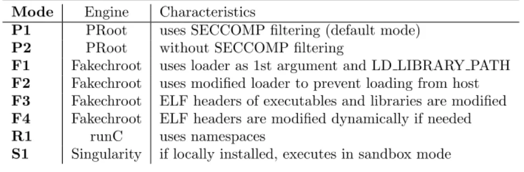
The S mode uses Singularity if locally installed. Mode Engine Characteristics
P1 PRoot uses SECCOMP filtering (default mode) P2 PRoot without SECCOMP filtering
F1 Fakechroot uses loader as 1st argument and LD LIBRARY PATH F2 Fakechroot uses modified loader to prevent loading from host F3 Fakechroot ELF headers of executables and libraries are modified F4 Fakechroot ELF headers are modified dynamically if needed
R1 runC uses namespaces
S1 Singularity if locally installed, executes in sandbox mode
Table 1: Execution modes.
The selection of a given execution mode is accomplished with the setup command as in the following example.
udocker setup --execmode=F3 container_name
3.2
Security
Since root privileges are not involved, any operation that requires such privileges will not be possible. The following are examples of operations that are not possible:
• Accessing host protected devices and files.
• Mount file-systems. • Change userid or groupid. • Change the system time.
• Change routing tables, firewall rules, or network interfaces.
The P and F modes do not provide isolation features such as the ones offered by Docker. If the containers content is not trusted then they should not be executed with these modes, as they will be executed inside the user environ-ment and can easily access host files and devices. The mode R1 provides better isolation by using namespaces.
The containers data is unpacked and stored in the user home directory or other location of choice. Therefore the containers data will be subjected to the same filesystem protections as other files owned by the user. If the con-tainers have sensitive information the files and directories should be adequately protected by the user.
In the following sections we describe three advanced scientific applications, widely used by the respective communities, in which the applicability of the developed solution is demonstrated.
4
Complex library dependencies: MasterCode
The current pattern of research activity in particle physics requires in many cases the use of complex computational frameworks, often characterized by being composed of different programs and libraries developed by independent groups. Moreover, in the past twenty years the average complexity of the standalone computational tools, which are part of these frameworks, has increased signif-icantly and nowadays they usually depend on a complex network of external libraries and dependencies.
At the same time, the computational resources required by physics studies have noticeably increased in comparison with the past and the use of computer clusters composed of hundreds, if not thousands, of nodes is now common. To address this issue, scientific collaborations split the computational load across different sites, whose operating system and software environment usually differs. As such, we investigate how the use of udocker could ease the deployment of complex scientific applications, allowing for an easy and fast setup across het-erogeneous systems. As an added value, we also observe that the use of exactly the same execution environment, where the application has supposedly been validated, protects against possible unexpected issues when moving between different sites with different compilers and libraries.
A prime example of modern complex applications is given by the frameworks used to perform global studies of particle physics models. The role of these applications, is to compare the theoretical predictions from hypothetical models with the observations performed by experiments, through probabilistic studies
(either frequentist or Bayesian), of the parameters that enter in the definition of these new models.
All should be done by thoroughly covering as many different measurements and observations as possible. Since new physics can manifest itself with different effects according to the specific experiment (or observation), it is not consistent to perform independent studies for each one separately.
On the computational side, this translates in the practical requirement of interfacing a plethora of different codes, each usually developed with the aim of computing the theoretical prediction of at most a few observables, with a frame-work that performs the comparison with experimental data and that manages the sampling of the parameter space.
Several groups in the particle physics community have developed their own independent frameworks [16, 17, 18, 19]. As a concrete example, for our studies, we consider MasterCode [16].
4.1
Code structure
As explained in the previous section, MasterCode depends on a wide range of external tools and libraries, which are tightly integrated into the main code-base. The full list of direct dependencies is the following:
• GNU autotools and GNU make.
• GNU toolchain (C/C++, Fortran77/90 compiler, linker, assembler). • wget, tar, find, patch.
• Python 2.7 or Python ≥ 3.3. • Cython ≥ 0.23 [20].
• ROOT ≥ 5 [21] and its dependencies. • numpy and its dependencies [22]. • Matplotlib [23] and its dependencies. • SQLite3.
• SLHAlib [24]. • MultiNest [25].
Moreover, it includes the following codes and their dependencies: • SoftSUSY [26].
• FeynWZ [27].
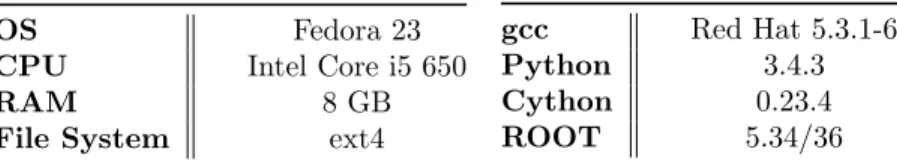
OS Fedora 23
CPU Intel Core i5 650
RAM 8 GB
File System ext4
Table 2: Test machine specifica-tions.
gcc Red Hat 5.3.1-6
Python 3.4.3
Cython 0.23.4
ROOT 5.34/36
Table 3: Software version of the most important tools and libraries used in our MasterCode bench-marks.
• micrOMEGAs [31]. • SSDARD [32]. • SDECAY [33]. • SuFla [34].
The GNU toolchain is required not only at compile-time but at run-time as well. Some of the applications used to compute the theoretical predictions are meta–codes that generate new code to be compiled and executed according to the parameter space point under analysis.
The capability of udocker in easing the use of MasterCode was tested, by building a Docker image based on Fedora 23, with all required libraries and tools installed. After, the image was deployed successfully at three different sites, where the physics analyses are usually run. We also successfully interfaced the execution of udocker with the local batch-systems.
To evaluate the performance impact of using udocker, we compared the compilation time of MasterCode with different setups, on a local workstation (see table 2 for the specifications).
4.2
Execution flow
The execution of a full analysis in MasterCode consists of three different different stages.
The first – and most complex – is the sampling of the parameter space of the model. In this phase of the execution, the MultiNest algorithm is used to sample the parameter space of the model. For each point in the parameter space, a call is made to each of the external codes used to compute the theo-retical predictions. The predictions are then compared with the experimental constraints and the likelihood of the point under analysis is computed. All the computed information is stored on the disk in an SQLite database for further analysis.
The main executable consists of a Python script that loads, through the ctypes interface, the MultiNest library, while Cython interfaces are used to
Sampling start
MultiNest selects a point
Run computer codes to compute physical observables
Compute χ2
Save data to storage using SQLite
convergence? No
Yes Sampling end
Figure 1: MasterCode execution flow during the sampling phase.
call the theory codes. Cython is also used to load an internal library, written in C++, that computes the likelihood (i.e. the χ2) of the point under scrutiny.
Important computational, I/O and storage resources are required for a fast execution of the sampling.
In practice, the parameter space of new physics models is usually too large to be sampled by a single instance of MasterCode. To overcome this obstacle, it is usually segmented in sub-spaces, for each one of which a separate sampling campaign is run. The execution flow is schematically depicted in fig. 1.
The second phase proceeds after the end of the sampling campaigns. The results of the various parameter–space sub–segments, stored in a large number of SQLite databases, are merged through the use of dedicated Python scripts. To reduce the total size of the dataset and ease the analysis phase a selection filter is applied to the sampled points. This step involves only I/O facilities and very often the performance limiting factor is the underlying file system.
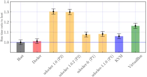
Host Dock er udo cker 1.0 (P2) udo cker 1.0.2 (P2) udo cker-fr (P1) udo cker-1.1.0 (P1) KVM VirtualBo x 1.0 1.1 1.2 1.3 1.4 Run time ratio to host
Figure 2: Compilation time for the MasterCode framework using the different setups we considered in our benchmark, averaged over ten repetitions of the benchmark and then shown as a ratio over the result obtained on the host. The black bars show the standard mean deviation. The color coding is the following: in gray we show the result obtained on the host machine. In orange we show the compilation time using different udocker setups. Red is used to show the Docker result, while blue and green are used to plot the performances of KVM and VirtualBox respectively.
The last stage is the physics analysis. In this step, one and two–dimensional ROOT histograms, defined for various physics observables and/or parameters, are filled with the likelihood information. From the computational perspective, it involves reading the databases produced in the previous step, whose size is commonly of the order of 10–50 GB (but can reach the terabyte for complex models), plus some lightweight computations to update the likelihood if needed.
4.3
Benchmarking udocker with MasterCode
To verify if the use of udocker has any significant performance impact on MasterCode, two benchmarks where performed in different environments:
• The compilation time of MasterCode.
• Comparison for a fixed pseudo-random number sequence, the running time for a restricted sampling of the so-called Constraint Minimal Supersym-metric Standard Model (CMSSM).
The environments that we considered for our comparison are: the bare host, three different versions of udocker, Docker, KVM and VirtualBox VMs.
Figure 2 shows the average compilation time of MasterCode over ten rep-etitions of the benchmark normalized to the native host result. The standard
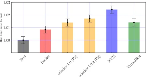
Host Dock er udo cker 1.0(P2) udo cker 1.0.2 (P2) KVM VirtualBo x 1.00 1.01 1.02 1.03 Run time ratio to host
Figure 3: Running time for a test MasterCode CMSSM sampling campaign, on our test machine, using different setups. Line colors and styling as in Figure 2.
mean deviation is shown in black on the top of each bar. The baseline host result is roughly ∼ 923 seconds. We notice that the first execution of the test is always the slowest, for all environments. This is due to I/O caching effects that disappear from the second iteration onward, where on the other hand we find a good stability. Indeed the standard deviation is small in all cases. From the results, we observe that udocker 1.0 and udocker 1.0.2 take a performance hit of about 30% with respect to the native host. Both these versions were run using the standard PROOT model without SECCOMP filtering. On the other hand, the newest udocker release, used with the SECCOMP filtering enabled, is only about 5% slower than the host and very close to the timing obtained in a KVM environment. The VirtualBox environment has a compilation time between the KVM and the old versions of udocker, with a performance hit of about 15%. The Docker environment is the very close to the native performance.
The results of the sampling-benchmark are shown in Figure 3, with the same format used for the compilation case. We performed the same sampling three times to avoid caching biases and statistical oscillations due to other background processes. The average running time for the native host is of ∼ 31187 seconds. We observe that all the different setups yield running times that are at most about 2.5% slower than the host machine. In this case, the slowest environment is the KVM one, while Docker is the fastest, with udocker (P2 mode) and KVM following very closely. The striking difference in the observed pattern with respect to the compilation–test case, is due to the fact that the sampling– phase is mostly CPU-bound, while the compilation–phase is mostly dependent on the I/O performances of the environment/system. Indeed, udocker, even in its default PROOT mode (without SECCOMP filtering), shows a negligible performance hit with respect to the native host.
5
MPI parallel execution: OpenQCD
In this section we describe how to use udocker to run MPI jobs in HPC systems. The process described applies both to interactive and batch–style job submis-sion, following the philosophy of udocker; it does not require any special user privileges, nor system administration intervention to setup.
We have chosen openQCD [35] to investigate both the applicability of our solutions and the effects of containerizing MPI processes on the performance of the code. The reason to choose this application stems from its high impact and the code features.
Regarding impact, Lattice QCD simulations spend every year hundreds of millions of CPU hours in HPC centers in Europe, USA and Japan. Current competitive simulations spread over thousands of processor cores. From the point of view of parallelization it requires only communication to nearest neigh-bors and thus, presents nice properties regarding scalability. OpenQCD is one of the most optimized codes available to run Lattice simulations and therefore, is widely distributed.
It is implemented using only open source software, may be downloaded and used under the license terms of the GPL model. Therefore it is an excellent laboratory for us to investigate with the required clarity the performance and applicability of our solution.
Competitive QCD simulations require latencies on the order of one microsec-ond, and Intranet bandwidths on the range 10–20 Gb/second in terms of effec-tive throughput. This is currently achieved only by the most modern Infiniband fabric interconnects (from QDR on). In what follows, we describe the steps to execute openQCD using udocker in a HPC system using Infiniband as low– latency interconnect. An analogous procedure can be followed for other MPI applications, also via simpler TCP/IP interconnects.
A container image of openQCD can be downloaded from the public Docker Hub repository1. From this image a container can be extracted to the filesystem with udocker create, as described before.
In the udocker approach the mpiexec of the Host machine is used to submit np MPI process instances as containers, in such a way that the containers are able to communicate via the Intranet fabric network (Infiniband in the case at hand).
For this approach to work, the code in the container needs to be compiled with the same version of MPI that is available in the HPC system. This is necessary because the Open MPI versions of mpiexec and orted available in the host system need to match with the compiled program. This limitation has to do with incompatibilities of the Open MPI libraries across different versions as well as with tight integration of Open MPI with the batch system.
The MPI job submission to the HPC cluster succeeds by issuing the following command:
$HOST_OPENMPI_BIN/mpiexec -np 128 udocker run \
--hostenv --hostauth --user=$USERID \ --workdir=$OPENQCD_CONTAINER_DIR \ openqcd \
$OPENQCD_CONTAINER_DIR/ym1 -i ym1.in Where the environment variable HOST OPENMPI BIN points to the location of the host MPI installation directory
Depending on the application and host operating system, a variable per-formance degradation may occur when using the default execution mode (Pn). In this situation other execution modes (such as Fn) may provide a significant higher performance
5.1
Scaling tests
In Figure 4 we plot the (weak) scaling performance of the most common oper-ation in QCD, that is, applying the so called Dirac Operator to a spinor field [36]. This operation can be seen as a sparse matrix–vector multiplication across the whole Lattice, of a matrix of dimension proportional to the Volume of the Lattice (12 × T × L3) times a vector of the same length.
The scaling properties have been measured in two different HPC systems: Altamira and CESGA2.
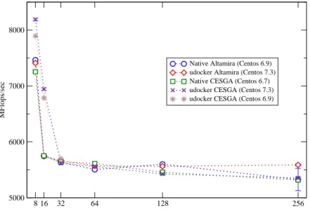
As can be observed the performance using udocker to run the MPI jobs is at the very least equal to the native performance. There are however a couple of observations to be made:
• At CESGA we observe that the performance of udocker is substantially better than the native performance when using 8 and 16 MPI processes, i.e., when the MPI processes spans only within one single node (the nodes at CESGA have 24 cores).
The host machine is running a CentOS 6.7 OS, while the container has a CentOS 7.3. We have checked, by running also the application with udocker in a CentOS 6.9 container, that this improvement is due to the improvement in the libraries of newer versions of CentOS. We actually ob-serve that the performance increases smoothly when increasing the version of CentOS.
More advanced versions of the libraries in the Operating System are able to make a more efficient usage of the shared memory capabilities of the CESGA nodes. We do not observe such improvement when the run is distributed over more than one node, in this case the effects of the intra-network communication overheads are likely dominating the performance. It is interesting to observe how the usage of containers can improve the applications performance when the underlying system has a somewhat older Operating System. This fact is specially relevant in most HPC
8 16 32 64 128 256 Number of cores 5000 6000 7000 8000 MFlops/sec
Native Altamira (Centos 6.9) udocker Altamira (Centos 7.3) Native CESGA (Centos 6.7) udocker CESGA (Centos 7.3) udocker CESGA (Centos 6.9)
Figure 4: Weak scaling analysis of the performance of the Lattice Dirac Operator (local lattice 324) using a containerized version of the application with udocker,
compared with the performance of the code used in the classical way (native performance). In these tests we have used P1 as execution mode. The results do not vary using F1.
centers that, for stability reasons, tend to have a very conservative policy when it comes to upgrading the underlying operating system and software. • In Altamira we observe a large dispersion in the performance results using 256 cores in native mode. The performance is much more stable using udocker. This can be traced down to local GPFS filesystem issues, which are more visible in the native run, as the system needs to look for the openMPI libraries across the filesystem, while with udocker the container has everything included in the $UDOCKER DIR directory.
Besides the scaling tests we also run openQCD for various settings of Lat-tice size and parameters, encountering no impact in performance in the time employed for each Hybrid MonteCarlo trajectory. This is of no surprise as I/O is not particularly intensive and frequent in Lattice QCD simulations: the usual checkpoints generate only Kbytes of data, while configurations, which in our Lattice sizes reached up to 1GB in size, are written in intervals of a few hours. For such I/O rates using udocker implies no penalty in performance.
Related to the above is the fact that in all the tests performed we have observed no performance difference between using P1 or F1 execution modes.
In summary, exploiting low-latency computing facilities using containers technology appears as an appealing possibility to maximize the efficiency on the use of resources, while guaranteeing researchers autonomy in profiting from modern system software capabilities.
6
Accessing GPGPUs: Modeling of
Biomolecu-lar Complexes
DisVis [37] and PowerFit [38] are two software packages for modeling biomolec-ular complexes. A detailed description of both software packages can be found in [39].
These software packages are coded in Python and are open source under the MIT license, published in github [40]. They leverage the use of GPGPUs through the OpenCL framework (PyOpenCL Python package) since the modeling uses the evaluation of Fast Fourier Transforms (FFTs), it uses the packages clFFT3
and gpyfft4.
Gromacs [41] is a versatile package to perform molecular dynamics, i.e. simu-late the Newtonian equations of motion for systems with hundreds to millions of particles. It is primarily designed for biochemical molecules like proteins, lipids and nucleic acids that have a complex bonded interactions, but since Gromacs is extremely fast at calculating the non–bonded interactions (that usually dom-inate simulations) many researchers are also using it for non–biological systems, such as polymers.
3https://github.com/clMathLibraries/clFFT
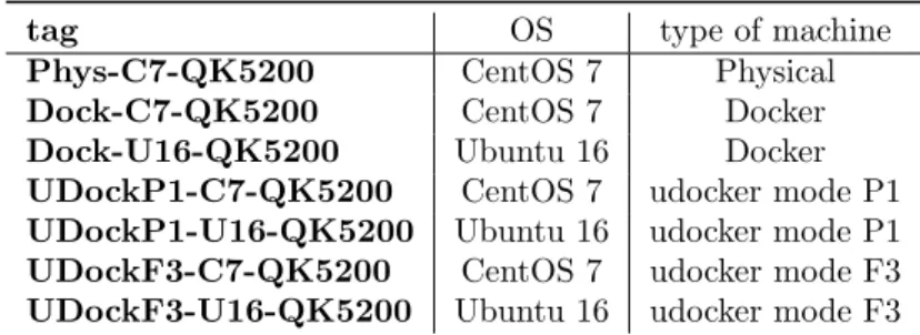
tag OS type of machine
Phys-C7-QK5200 CentOS 7 Physical
Dock-C7-QK5200 CentOS 7 Docker
Dock-U16-QK5200 Ubuntu 16 Docker
UDockP1-C7-QK5200 CentOS 7 udocker mode P1 UDockP1-U16-QK5200 Ubuntu 16 udocker mode P1 UDockF3-C7-QK5200 CentOS 7 udocker mode F3 UDockF3-U16-QK5200 Ubuntu 16 udocker mode F3
Table 4: Execution environments for the DisVis and Gromacs applications.
6.1
Setup and deployment
The physical host used to benchmark udocker with the DisVis and Gromacs applications using GPGPUs was made available by the Portuguese National Distributed Computing Infrastructure (INCD). It is hosted at the INCD main datacenter in Lisbon and its characteristics are described in the Appendix.
The applications DisVis v2.0.0 and Gromacs 2016.3 were used. Docker im-ages were built from Dockerfiles for both applications and for two operating sys-tems: CentOS 7.3 (Python 2.7.5, gcc 4.8.5) and Ubuntu 16.04 (Python 2.7.12, gcc 5.4.0), the versions of the applications in the Docker images are the same as in the physical host.
The applications in the Docker images were built with GPGPU support and the NVIDIA software that matches the same version of the NVIDIA driver deployed in the physical host system.
Those same images were then used to perform the benchmarks using both Docker and udocker. In particular, udocker has several modes of execution (c.f. the user manual hosted at [9]), available through the setup --execmode option. Two such options have been chosen for Gromacs execution, namely: P1 corresponding to PRoot with SECCOMP filtering and F3 corresponding to Fakechroot with maximum isolation from the host system. For DisVis we only used the P1 execution mode.
Table 4 summarizes the different execution environments used in the bench-marks in terms of operating system and type of machine: physical (the host), Docker or udocker. The tags UDockP1 and UDockF3 correspond to the two chosen execution modes of udocker mentioned above.
6.2
Benchmark results
The DisVis use case was executed with input molecule PRE5-PUP2 complex. The application is executed with one GPU (the option -g selects the GPU execution mode), using the following command:
$shell> disvis O14250.pdb \ Q9UT97.pdb \
Phys-C7 Dock-C7 Dock-U16 UDockP1-C7 UDockP1-U16 Machine 0.90 0.92 0.94 0.96 0.98 1.00 1.02 1.04
Ratio Run time
Disvis: case = PRE5-PUP2-complex Angle = 5.0 Voxelspacing = 1 GPU = QK5200
Ratio
Figure 5: Ratio between runtime values of Docker or udocker and the physical host of the DisVis use case. Lower values indicate better performance.
restraints.dat \ --angle 5.0 \ --voxelspacing 1 \ -g \
-d ${OUT_DIR}
The Gromacs gmx mdrun was executed with an input file of the amyloid beta peptide molecule. The application is executed with one GPU and 8 OpenMP threads (per MPI rank), using the following command:
$shell> gmx mdrun -s md.tpr \ -ntomp 8 \ -gpu_id 0
For each case, 20 runs have been executed for statistical purposes. The run time of each execution is recorded and a statistical analysis is done as follows: The outliers are detected and masked from the sample of 20 points, then the average and standard deviation are calculated for each case and environment option (physical host, Docker or udocker). The ratio between the average run time of each docker or udocker environment with the average run time in the physical host is plotted in Figures 5 and 6. Typical execution times for both cases range between 20 and 30 minutes.
The first ratio (column) in each figure is 1 since the baseline is the physical host, the standard deviation of the ratio is calculated based on the statistical formula for the ratio of two variables:
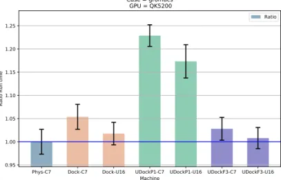
Phys-C7 Dock-C7 Dock-U16 UDockP1-C7 UDockP1-U16 UDockF3-C7 UDockF3-U16 Machine 0.95 1.00 1.05 1.10 1.15 1.20 1.25
Ratio Run time
Case = gromacs GPU = QK5200
Ratio
Figure 6: Ratio between runtime values of Docker or udocker and the physical machine of the Gromacs use case. Lower values indicate better performance.
∆R = ti/thost×
p
(∆ti/ti)2+ (∆thost/thost)2 (1)
Where: tiis the average runtime in a given environment, thostis the average
runtime in the physical host, ∆thost and ∆ti are the corresponded standard
deviations.
Figure 5 correspond to the benchmark of the DisVis use case. It can be seen that the execution of both Docker and udocker in CentOS 7.3 containers although 1 − 2% smaller than 1 is still compatible with this value. This shows that executing the application in this type of virtualized environment has the same performance as executing it in the physical host. On the other hand executing the application in the Ubuntu 16.04 containers (both Docker and udocker cases) the execution time is around 5% better than in the physical host.
Figure 6 correspond to the benchmark of the Gromacs use case. It can be seen that the execution in CentOS 7.3 containers for Docker (second bar) and udocker with execution mode F3 (Fakechroot with maximum isolation from the host system, sixth bar), are 3–5% worse than the execution in the physical host although still compatible with one due to the statistical error. Also in the case of execution in Ubuntu 16.04 containers (third and seventh bars) the ratios are compatible with one, i.e. the containerized application execution has the same performance as in the physical host. In the case of executing the application in udocker containers with execution mode P1 (PRoot with SECCOMP filtering, forth and fifth bars), a penalty in performance of up to 22% is observed.
for the Gromacs use case can be explained by the computational model itself, since Gromacs is using the GPGPU and 8 OpenMP threads (corresponding to 8 CPU cores) frequent exchanges of data between the GPGPU and the CPU threads and possible context change between CPU tasks translate into a perfor-mance penalty in the P1 execution mode that does not occur in the F3 execution mode. This is partially confirmed by comparing to the DisVis use case that uses almost exclusively the GPGPU (and at most only 1 CPU) where the P1 execu-tion mode does not have any impact on performance.
7
Conclusions
In this paper we have described a middleware suite that provides full autonomy to the user when it comes to execute applications in Docker container format. We have shown that our solution provides a complete encapsulation of the soft-ware, without significantly impacting performance.
In this paper we have analyzed a number of differently oriented use cases, and got clear evidence that compute intensive applications pay practically no perfor-mance penalty when executed as udocker containers. Regarding I/O bounded applications, the udocker execution modes Pn introduce a penalty that can be largely minimized by using the Fn execution modes. The small penalty still observed with the Fn modes is introduced by the filename translation, the data access itself is unaffected. Other tools such as Singularity or Shifter can mount container images as file systems keeping many file system calls local. Mounting the images may yield better performance especially when using a shared net-work file system, however this has the disadvantage of requiring privileges. All OpenQCD performance measurements in this paper were performed with the container image placed in Lustre file systems without any noticeable impact in comparison with native execution.
Tools like udocker are essential when it comes to access external computing resources with different execution environments. It is particularly so when ac-cessing cloud infrastructures and shared computing infrastructures such as HPC clusters, where running software with encapsulation is a necessity to remain in-dependent of the host computing environment. Users of DisVis and PowerFit have been running these applications in the EGI Grid infrastructure at sites offering GPGPU resources, using udocker and performing grid job submission as any other application. udocker empowers users to execute applications en-capsulated in Docker containers in such systems in a fully autonomous way.
Since its first release in June 2016 udocker expanded quickly in the open source community as can be seen from the github metrics (number of stars, forks or number of external contributions). Since then it has been used in large international collaborations like the case of MasterCode reported here.
The extra flexibility offered by udocker has made it a very appreciated tool, and has been already adopted by a number software projects to
comple-ment Docker. Among them openmole5, bioconda6, common-workflow-language (cwl)[42] or SCAR - Serverless Container-aware ARchitectures7.
Acknowledgements
This work has been performed in the framework of the H2020 project INDIGO-Datacloud (RIA 653549). The work of E.B. is supported by the Collaborative Research Center SFB676 of the DFG, “Particles, Strings and the early Uni-verse”. The proofs of concept presented have been performed at the FinisTerrae II machine provided by CESGA (funded by Xunta de Galicia and MINECO), at the Altamira machine (funded by the University of Cantabria and MINECO) and at the INCD-Infraestrutura Nacional de Computa¸c˜ao Distribu´ıda (funded by FCT, P2020, Lisboa2020, COMPETE and FEDER under the project number 22153-01/SAICT/2016).
We are indebted to the managers of these infrastructures for their generous support and constant encouragement.
5https://www.openmole.org/api/index.html#org.openmole.plugin.task.udocker.package
6https://anaconda.org/bioconda/udocker
Appendix: Hardware and Software setup
The images of the containers used in this work are publicly available in the Docker hub, at the following urls:
• OpenQCD: https://hub.docker.com/r/iscampos/openqcd/ • DISVIS: https://hub.docker.com/r/indigodatacloudapps/disvis • POWERFIT: https://hub.docker.com/r/indigodatacloudapps/powerfit
• MASTERCODE: https://hub.docker.com/r/indigodatacloud/docker-mastercode/ The proofs of concept presented have been carried out in the following infras-tructures, with the following Hardware/OS/Software setup:
• Finisterrae-II - CESGA, Santiago de Compostela
https://www.cesga.es/es/infraestructuras/computacion/FinisTerrae2 Hardware Setup:
– Processor type Intel(R) Xeon(R) CPU E5-2680 v3 @ 2.50GHz, with cache size 30MB
– Node configuration 2 CPUs Haswell 2680v3, (2x12 = 24 cores/node) and 128GB RAM/node
– Infiniband Network Mellanox Infiniband FDR@56Gbps Software setup:
– Operating System CentOS 6 – Compilers GCC 6.3.0 – MPI libraries openmpi/2.0.2 • Altamira - IFCA-CSIC, Santander
https://grid.ifca.es/wiki/Supercomputing/Userguide Hardware Setup:
– Processor type Intel(R) Xeon(R) CPU E5-2670 0 @ 2.60GHz, with cache size 20MB.
– Node configuration 2 CPUs E5-2670, (2x8 = 16 cores/node) and 64GB RAM/node
– Infiniband Network Mellanox Infiniband FDR@56Gbps Operating system and Software setup:
– Operating System CentOS 6 – Compilers GCC 5.3.0 – MPI libraries openMPI/1.8.3 • INCD, Lisbon
https://www.incd.pt Hardware Setup:
– Processor type Intel(R) Xeon(R) CPU E5-2650L v3 @ 1.80GHz
– Node configuration 2 CPUs (2x12 = 24 cores/node x2 = 48 in HiperThread-ing mode) and 192GB RAM
– GPU model NVIDIA Quadro K5200 Operating system and Software setup:
– Operating System CentOS 7.3 – NVIDIA driver 375.26
– CUDA 8.0.44 – docker-engine 1.9.0 – udocker 1.0.3
References
[1] Linus Torvalds (2015). Linux Operating system.
Can be retrieved from https://github.com/torvalds/linux/ [2] P. Menage
https://www.kernel.org/doc/Documentation/cgroup-v1/cgroups.txt [3] See https://en.wikipedia.org/wiki/Linux namespaces
[4] See eg. https://www.freebsd.org/doc/handbook/jails.html [5] S. Hykes (Docker Inc)
See software description and downloads in http://www.docker.com [6] Description of the cloud-based Docker repository service can be found in:
https://www.docker.com/products/docker-hub
[7] Kurtzer GM, Sochat V, Bauer MW (2017) Singularity: Scientific containers for mobility of compute. PLOS ONE 12(5): e0177459. https://doi.org/10.1371/journal.pone.0177459
[8] Jacobsen, Douglas M. and Richard Shane Canon. Contain This, Unleashing Docker for HPC. (2015).
[9] udocker can be downloaded from https://github.com/indigo-dc/udocker [10] Quigley, David et al. Unionfs: User- and Community-Oriented
Develop-ment of a Unification File System. (2006). [11] See https://proot-me.github.io/
[12] See https://github.com/dex4er/fakechroot [13] See https://nixos.org/patchelf.html
[14] See https://github.com/opencontainers/runc [15] See https://www.opencontainers.org
[16] K. J. de Vries, PhD thesis Global Fits of Supersymmetric Models af-ter LHC Run 1 (2015), available on the Imperial College website: http://hdl.handle.net/10044/1/27056.
[17] L. Roszkowski, R. Ruiz de Austri, J. Silk and R. Trotta, Phys. Lett. B 671 (2009) 10 doi:10.1016/j.physletb.2008.11.061 [arXiv:0707.0622 [astro-ph]]. [18] P. Bechtle, K. Desch and P. Wienemann, Comput. Phys. Commun. 174
(2006) 47 doi:10.1016/j.cpc.2005.09.002 [hep-ph/0412012].
[19] L. Roszkowski, R. Ruiz de Austri, J. Silk and R. Trotta, Phys. Lett. B 671 (2009) 10 doi:10.1016/j.physletb.2008.11.061 [arXiv:0707.0622 [astro-ph]]. [20] Behnel, S. and Bradshaw, R. and Citro, C. and Dalcin, L. and Seljebotn,
D.S. and Smith, K., “Cython: The Best of Both Worlds”, Computing in Science & Engineering 13.2 (2011): 31-39, 10.1109/MCSE.2010.118. [21] R. Brun and F. Rademakers, “ROOT: An object oriented data analysis
framework,” Nucl. Instrum. Meth. A 389 (1997) 81. doi:10.1016/S0168-9002(97)00048-X
[22] Walt, S. V. D., Colbert, S. C., & Varoquaux, G. (2011), “The NumPy array: a structure for efficient numerical computation.”, Computing in Science & Engineering, 13(2), 22-30.
[23] Hunter, J. D. (2007), “Matplotlib: A 2D graphics environment”, Comput-ing In Science & EngineerComput-ing, 9(3), 90-95.
[24] T. Hahn, Comput. Phys. Commun. 180 (2009) 1681 doi:10.1016/j.cpc.2009.03.012
[25] F. Feroz, M. P. Hobson and M. Bridges, Mon. Not. Roy. Astron. Soc. 398 (2009) 1601 doi:10.1111/j.1365-2966.2009.14548.x [arXiv:0809.3437 [astro-ph]].
[26] B. C. Allanach, Comput. Phys. Commun. 143 (2002) 305 doi:10.1016/S0010-4655(01)00460-X [hep-ph/0104145].
[27] S. Heinemeyer et al., JHEP 0608 (2006) 052 [arXiv:hep-ph/0604147]; S. Heinemeyer, W. Hollik, A. M. Weber and G. Weiglein, JHEP 0804 (2008) 039 [arXiv:0710.2972 [hep-ph]].
[28] S. Heinemeyer, W. Hollik and G. Weiglein, Comput. Phys. Commun. 124 (2000) 76 [arXiv:hep-ph/9812320]; S. Heinemeyer, W. Hollik and G. Wei-glein, Eur. Phys. J. C 9 (1999) 343 [arXiv:hep-ph/9812472]; G. Degrassi, S. Heinemeyer, W. Hollik, P. Slavich and G. Weiglein, Eur. Phys. J. C 28 (2003) 133 [arXiv:hep-ph/0212020]; M. Frank et al., JHEP 0702 (2007) 047 [arXiv:hep-ph/0611326]; T. Hahn, S. Heinemeyer, W. Hollik, H. Rzehak and G. Weiglein, Comput. Phys. Commun. 180 (2009) 1426; T. Hahn, S. Heinemeyer, W. Hollik, H. Rzehak and G. Weiglein, Phys. Rev. Lett. 112 (2014) 14, 141801 [arXiv:1312.4937 [hep-ph]]; H. Bahl and W. Hollik, Eur. Phys. J. C 76 (2016) 499 [arXiv:1608.01880 [hep-ph]]. See http://www.feynhiggs.de .
[29] P. Bechtle, O. Brein, S. Heinemeyer, G. Weiglein and K. E. Williams, Com-put. Phys. Commun. 181 (2010) 138 [arXiv:0811.4169 [hep-ph]], ComCom-put. Phys. Commun. 182 (2011) 2605 [arXiv:1102.1898 [hep-ph]]; P. Bechtle et al., Eur. Phys. J. C 74 (2014) 3, 2693 [arXiv:1311.0055 [hep-ph]]; P. Bech-tle, S. Heinemeyer, O. St˚al, T. Stefaniak and G. Weiglein, Eur. Phys. J. C 75 (2015) no.9, 421 [arXiv:1507.06706 [hep-ph]].
[30] P. Bechtle, S. Heinemeyer, O. St˚al, T. Stefaniak and G. Weiglein, Eur. Phys. J. C 74 (2014) 2, 2711 [arXiv:1305.1933 [hep-ph]]; JHEP 1411 (2014) 039 [arXiv:1403.1582 [hep-ph]].
[31] G. Belanger, F. Boudjema, A. Pukhov and A. Semenov, Comput. Phys. Commun. 185 (2014) 960 [arXiv:1305.0237 [hep-ph]], and references therein.
[32] Information about this code is available from K. A. Olive: it contains important contributions from J. Evans, T. Falk, A. Ferstl, G. Ganis, F. Luo, A. Mustafayev, J. McDonald, F. Luo, K. A. Olive, P. Sandick, Y. Santoso, C. Savage, V. Spanos and M. Srednicki.
[33] M. Muhlleitner, A. Djouadi and Y. Mambrini, Comput. Phys. Commun. 168 (2005) 46 [hep-ph/0311167].
[34] G. Isidori and P. Paradisi, Phys. Lett. B 639 (2006) 499 [arXiv:hep-ph/0605012]; G. Isidori, F. Mescia, P. Paradisi and D. Temes, Phys. Rev. D 75 (2007) 115019 [arXiv:hep-ph/0703035], and references therein. [35] Martin L¨uscher,
Code available at: http://luscher.web.cern.ch/luscher/openQCD [36] Martin L¨uscher,
Lectures given at the Summer School on Modern perspectives in lattice QCD, Les Houches, August 3-28 (2009)
[37] G.C.P. Van Zundert, A.M.J.J. Bonvin, DisVis: quantifying and visualizing the accessible interaction space of distancerestrained biomolecular com-plexes, Bioinformatics 31 (2015) 3222–3224
[38] G.C.P. Van Zundert, A.M.J.J. Bonvin, Fast and sensitive rigid-body fitting into cryo-EM density maps with PowerFit, AIMS Biophys. 2 (2015) 73–87. [39] G.C.P. van Zundert, et al., The DisVis and PowerFit Web Servers: Explo-rative and IntegExplo-rative Modeling of Biomolecular Complexes, J. Mol. Biol. (2016), http://dx.doi.org/10.1016/j.jmb.2016.11.032
[40] DisVis: https://github.com/haddocking/disvis PowerFit: https://github.com/haddocking/powerfit
[41] Abraham, M. J., et al., GROMACS: High performance molecular simula-tions through multi-level parallelism from laptops to supercomputers, Soft-wareX 2015, 1–2, 19– 25 DOI: 10.1016/j.softx.2015.06.001
[42] Peter Amstutz, Michael R. Crusoe, Nebojˇsa Tijani´c (editors), Brad Chap-man, John Chilton, Michael Heuer, Andrey Kartashov, Dan Leehr, Herv´e M´enager, Maya Nedeljkovich, Matt Scales, Stian Soiland-Reyes, Luka Sto-janovic
Common Workflow Language, v1.0. Specification, Common Workflow Lan-guage working group (2016). https://w3id.org/cwl/v1.0/