www.hydrol-earth-syst-sci.net/20/4895/2016/ doi:10.5194/hess-20-4895-2016
© Author(s) 2016. CC Attribution 3.0 License.
Assimilation of SMOS brightness temperatures or soil moisture
retrievals into a land surface model
Gabriëlle J. M. De Lannoy1and Rolf H. Reichle2
1KU Leuven, Department of Earth and Environmental Sciences, Heverlee, Belgium
2NASA Goddard Space Flight Center, Global Modeling and Assimilation Office, Greenbelt, Maryland, USA
Correspondence to:Gabriëlle J. M. De Lannoy ([email protected])
Received: 16 August 2016 – Published in Hydrol. Earth Syst. Sci. Discuss.: 23 August 2016 Revised: 8 November 2016 – Accepted: 27 November 2016 – Published: 15 December 2016
Abstract.Three different data products from the Soil Mois-ture Ocean Salinity (SMOS) mission are assimilated sepa-rately into the Goddard Earth Observing System Model, ver-sion 5 (GEOS-5) to improve estimates of surface and root-zone soil moisture. The first product consists of multi-angle, dual-polarization brightness temperature (Tb) observations at the bottom of the atmosphere extracted from Level 1 data. The second product is a derived SMOS Tb product that mim-ics the data at a 40◦incidence angle from the Soil Moisture Active Passive (SMAP) mission. The third product is the op-erational SMOS Level 2 surface soil moisture (SM) retrieval product. The assimilation system uses a spatially distributed ensemble Kalman filter (EnKF) with seasonally varying cli-matological bias mitigation for Tb assimilation, whereas a time-invariant cumulative density function matching is used for SM retrieval assimilation. All assimilation experiments improve the soil moisture estimates compared to model-only simulations in terms of unbiased root-mean-square differ-ences and anomaly correlations during the period from 1 July 2010 to 1 May 2015 and for 187 sites across the US. Especially in areas where the satellite data are most sensi-tive to surface soil moisture, large skill improvements (e.g., an increase in the anomaly correlation by 0.1) are found in the surface soil moisture. The domain-average surface and root-zone skill metrics are similar among the various assim-ilation experiments, but large differences in skill are found locally. The observation-minus-forecast residuals and analy-sis increments reveal large differences in how the observa-tions add value in the Tb and SM retrieval assimilation sys-tems. The distinct patterns of these diagnostics in the two systems reflect observation and model errors patterns that
are not well captured in the assigned EnKF error parameters. Consequently, a localized optimization of the EnKF error pa-rameters is needed to further improve Tb or SM retrieval as-similation.
1 Introduction
Microwave satellite missions are collecting large amounts of data for soil moisture monitoring. It is not yet clear, how-ever, how this wealth of data can be used in the most effi-cient way to obtain global estimates of soil moisture that can improve, e.g., weather prediction, flood and drought model-ing, agricultural yield monitormodel-ing, or landslide predictions. Many such applications require knowledge of soil moisture in a deeper layer, where water is extracted by plant roots or stored to buffer drainage and runoff, not the approximately 5 cm surface layer to which the current L-band (∼1.4 GHz) microwave missions are sensitive. Moreover, L-band satel-lite observations have a fairly coarse spatial resolution (about 40 km) and are available only at particular overpass times, typically once every 2–3 days for a given location. The chal-lenge is thus to derive soil profile moisture information at all times and locations through data assimilation, that is, through the merger of satellite observations with information from a dynamical land surface model.
(L1) brightness temperature (Tb) data, Level 2 (L2) surface soil moisture (SM) retrievals, and derived Level 3 (L3) prod-ucts. The SMAP mission also provides an operational Level 4 surface and root-zone soil moisture product (L4_SM; En-tekhabi et al., 2014; Reichle et al., 2016) that is based on the assimilation of L1 SMAP Tb data into Goddard Earth Observing System Model, version 5 (GEOS-5) land surface simulations. Alternatively, a soil moisture assimilation sys-tem could ingest L2 SM retrievals instead of L1 Tb observa-tions.
In this paper, we compare Tb and SM retrieval assimi-lation using a historical (5-year) record of SMOS observa-tions over North America in an assimilation system similar to that of the SMAP L4_SM system. The main differences between the SMAP L4_SM system and the experiments in this paper pertain to the differences in assimilated data, to the difference in spatial resolution of the resulting soil mois-ture products (36 km in the current paper; see below; 9 km for the L4_SM product), and to differences in meteorological forcing input (re-analysis meteorology in the current paper; operational forecast meteorology corrected with gauge-based precipitation in the L4_SM product).
It is more difficult to assimilate Tb observations than SM retrievals because brightness temperatures are only indirectly connected with the land surface variables of interest and the Tb data come in multiple polarizations. SMOS Tb observa-tions are even more complex because of their multi-angular nature. Some of the SMOS L1 Tb data complexity is re-duced in the L3 SMOS Tb product and further addressed in Munoz-Sabater et al. (2014) and De Lannoy et al. (2015), who prepared the L1 SMOS Tb data for assimilation into (quasi-)operational systems.
Successful examples of SMOS Tb assimilation using a va-riety of simplifying assumptions are illustrated in Lievens et al. (2015); De Lannoy and Reichle (2016); Kornelsen et al. (2016). These studies use a radiative transfer model (RTM) to dynamically invert Tb information into corrections to mod-eled soil moisture estimates. In this paper, we advance the spatially distributed multi-angle and dual-polarization Tb as-similation of De Lannoy and Reichle (2016) in the GEOS-5 land surface model with a new version of Tb observations and an improved spatial support and forward simulation of the Tb observation predictions. Moreover, to mimic SMAP Tb assimilation we also assimilate dual-polarization single-angle 40◦SMOS Tb observations after fitting the multi-angle Tb data (De Lannoy et al., 2015).
A key disadvantage of a system that assimilates SM re-trievals is that the SM rere-trievals may be produced with incon-sistent ancillary data, such as for example soil temperature simulated by another model than that used in the assimila-tion system. The current SMOS SM retrievals by themselves have been found to be skillful (Al-Yaari et al., 2014; Fascetti et al., 2016), and research is ongoing to further improve them (Rodriguez-Fernandez et al., 2015; Ye et al., 2015; Zhao et al., 2015; van der Schalie et al., 2016; Wigneron et al.,
2016). The use of these SMOS SM retrievals has been mani-fold, e.g., to derive enhanced estimates of precipitation (Wan-ders et al., 2015; Koster et al., 2016), to derive offline root-zone soil moisture estimates (Ford et al., 2014), or to of-fline downscale the data to higher-resolution soil moisture estimates (Piles et al., 2014). Other studies have assimilated SMOS SM retrievals online into land surface models to pos-sibly downscale the retrievals and consistently improve soil moisture and other land surface variables (Ridler et al., 2014; Zhao et al., 2014; Lievens et al., 2015), leading to, e.g., im-proved estimates of floods (Alvarez-Garreton et al., 2015) and crop growth (Chakrabart et al., 2014). In this paper, we use a spatially distributed assimilation system to integrate SMOS SM retrievals into the GEOS-5 land surface model with the aim of inferring improved surface and root-zone soil moisture estimates. Our study mainly differs from the above SMOS SM retrieval studies in the continental and multi-year scale of the experiments, in the advanced quality screening and spatial support of the SM retrieval observations, and in the comparison between Tb and SM retrieval assimilation (also discussed in Lievens et al., 2015).
To assess the potential of Tb and SM retrieval assimilation, 5 years of SMOS Tb data or SM data are assimilated into the GEOS-5 land surface model using a careful data quality control and data preprocessing. The observations are associ-ated with a realistic antenna pattern, containing 50 % of the signal power in a circular area with 20 km radius. Special attention is paid to large-scale patterns of random and per-sistent forecast and observation errors in the different assim-ilation systems, and to the impact of the different assimila-tion schemes on the skill of surface and root-zone soil mois-ture estimates. Section 2 describes the SMOS observations, the various modeling components, and the in situ validation data. Section 3 highlights the technical differences between the various assimilation schemes, and Sect. 4 presents the re-sults.
2 Data and model
2.1 SMOS Tb observations
Figure 1.Flowchart of Tb assimilation. The forward simulation consists of(a)land surface model simulations and(b)Tb simulations on the 36 km EASEv2 grid. The Tb simulations are subsequently(c)aggregated using weights based on an approximate antenna pattern. The resulting footprint-scale brightness temperature observation predictions are compared to(d)SMOS observations to calculate innovations (O–F) at the footprint scale.(e)The three-dimensional EnKF maps the footprint-scale innovations to the 36 km EASEv2 grid based on the modeled error correlations between the footprint-scale Tb and the 36 km soil moisture and soil temperature state variables (per Eqs. 1 and 2).
too sensitive (R. Oliva and Y. Kerr, personal communica-tion, 2016). After the initial screening, we correct the L1 Tb values for geometric and Faraday rotation and for atmo-spheric and reflected extraterrestrial radiation (De Lannoy et al., 2015) using Modern-Era Retrospective Analysis for Research and Applications (MERRA) version 2 (MERRA2; Bosilovich et al., 2015) background fields. The resulting Tb values at the bottom of the atmosphere are then binned into 41 evenly spaced angular bins with the center angle ranging from 20 through 60◦. Next, the data are regridded from the 15 km discrete global grid (DGG) on which they are posted to the 36 km cylindrical Equal-Area Scalable Earth (EASEv2) grid (Brodzik et al., 2014), and the data are screened for ex-cessive sub-36 km heterogeneity (spatial standard deviation >7 K), which is indicative of open water bodies or RFI. Tb values for a given 36 km EASEv2 grid cell are computed only if at least two valid DGG observations are available.
From these preprocessed Tb data, two datasets are derived for assimilation: (i) a seven-angle Tb dataset, with incidence angles θ=[30, 35, 40, 45, 50, 55, 60◦] (De Lannoy et al., 2013), and (ii) a fitted Tb dataset (De Lannoy et al., 2015) from which only the Tb at a 40◦incidence angle is used to mimic the single-angle nature of SMAP Tb observations. We refer to these datasets as Tb_7ang and Tb_fit, respectively. Tb_fit data are only retained when the fitting error is less than 5 K and a minimum of 15 data points contribute to the entire fitted angular signature, with at least 5 data points above and
below the 40◦incidence angle and at least 10 data points in the incidence angle interval between 30 and 50◦.
2.2 SMOS SM retrieval observations
devi-ation>0.2 m3m−3). SM values for a given 36 km EASEv2 grid cell are computed only if at least two valid DGG obser-vations are available.
2.3 Soil moisture and brightness temperature modeling The land data assimilation system used here employs the GEOS-5 catchment land surface model (CLSM; Koster et al., 2000), along with an L-band tau-omega radiative transfer model (RTM; De Lannoy et al., 2013, 2014b). The CLSM simulations use GEOS-5 parameters (Mahanama et al., 2015; De Lannoy et al., 2014a) similar to those used in the SMAP L4_SM product, and are forced with 1/2◦×2/3◦GEOS-5 forcing data from MERRA (Rienecker et al., 2011) bilinearly interpolated to the model grid. The study domain covers most of North America, with the northwestern corner at (125◦W, 55◦N) and the southeastern corner at (60◦W, 24◦N).
The computational elements are the 36 km EASEv2 grid cells. The land model computation time step is 7.5 min, and output is saved at 3 h intervals. At each grid cell, the sur-face soil moisture content (sfmc, 0–5 cm) and root-zone soil moisture content (rzmc, 0–100 cm) are diagnosed based on three prognostic variables: catchment deficit (catdef), root-zone excess (rzexc), and surface excess (srfexc). Similarly, the surface (skin) temperature is diagnosed from the prog-nostic land surface temperatures across the saturated (tc1), unsaturated (tc2), and wilting (tc4) sub-grid areas. Finally, the soil temperature (tp1 for the topmost layer) is diagnosed from the prognostic ground heat content (ght1 for the top layer). An overview of the model variables is given in Re-ichle et al. (2015); Koster et al. (2000) and Ducharne et al. (2000).
The L-band tau-omega RTM converts the 36 km CLSM soil moisture and temperature simulations into 36 km L-band Tb estimates when the soil is not frozen or covered with snow, when precipitation is less than 10 mm day−1, and where the open water fraction is less than 5 %. For each 36 km grid cell, key parameters of the RTM are estimated by minimizing Eq. (B.1) in De Lannoy et al. (2014b), using a 5-year history of SMOS v620 Tb data, and computing obser-vation predictions (see below) at the footprint scale. Specif-ically, all 36 km grid cells within one footprint area are ini-tially assigned the same set of RTM parameters, while the dynamic background information is spatially variable. For each 36 km grid cell, the calibration estimates a spatially ho-mogeneous set of RTM parameters for the entire associated footprint area, and the resulting values are assigned to the central (and typically dominant) 36 km grid cell only. For the forward calculation of the Tb observation predictions during the data assimilation, all 36 km pixels have a unique set of RTM parameters. The RTM is calibrated using all 5 years of available Tb data and aims at minimizing climatologi-cal biases. The data assimilation is performed over the same 5 years and aims at addressing random (or short-term) errors. The methodology is very similar to that in De Lannoy and
Reichle (2016), but with the difference that, here, the RTM does not simulate atmospheric contributions (because the Tb observations are now a priori corrected for atmospheric con-tributions) and the observation predictions are now spatially aggregated using a realistic (but approximate) antenna pat-tern.
For the computation of differences between SMOS obser-vations and footprint-scale model simulations in the RTM calibration and for the computation of the “observation-minus-forecast” (O–F) residuals in the assimilation system (Sect. 3.1, Fig. 1), the modeled 36 km soil moisture or Tb simulations are aggregated to the footprint scale by spa-tial convolution with weights given by an approximation of the SMOS antenna pattern. We also refer to these spa-tially aggregated model estimates as “observation predic-tions”. The SMOS antenna pattern is approximated by a two-dimensional Gaussian function containing 50 % of the signal within a circle with a radius of 20 km. The simulations out-side a radius of 40 km are discarded in the computation of the footprint-scale estimates.
The number of 36 km EASEv2 grid cells included in one footprint area varies with latitude. The circular footprint shape is preserved everywhere on the globe. In contrast, the shape of the EASEv2 grid cells projected on the globe varies with the latitude, with an aspect ratio of 1 at 30◦ (north– south) latitude, larger than 1 towards the poles and less than 1 towards the Equator. Therefore, at higher latitudes multiple EASEv2 grid cells with the same latitude and various longi-tudes belong to one circular footprint, whereas towards the Equator, several EASEv2 grid cells with the same longitude and various latitudes contribute to the footprint. Overall, the difference between single 36 km simulations and footprint-scale values is small, but the number of valid Tb observa-tion predicobserva-tions at the footprint scale is reduced, because of the increased likelihood of finding a 36 km grid cell with a non-negligible water fraction, snow amount, or precipitation within the footprint area.
2.4 In situ soil moisture data and metrics
using all 3 h forecast and analysis time steps in the period 1 July 2010–1 May 2015, excluding times when the soil is frozen (top layer soil temperature<274.15 K) or snow cov-ered (snow water equivalent>0 kg m−2). The anomaly cor-relation is based on anomaly time series obtained by subtract-ing a multi-year smoothed climatology from both the simula-tions and in situ observasimula-tions. Note that the assimilation and open-loop simulations have, by design, the same climatolog-ical variability; the assimilation only corrects for random er-rors. Metrics at a single site are only calculated if at least 200 data points are available. Skill metrics across an entire network are calculated by clustering the sites within SCAN and USCRN to avoid densely sampled areas dominating the validation metrics and to ensure realistic confidence inter-vals (De Lannoy and Reichle, 2016). The number of clusters is estimated a priori after prescribing an average cluster ra-dius of 3◦, which approximately reflects the autocorrelation length of large-scale topographic and meteorological phe-nomena, or of large-scale soil moisture patterns (Vinnikov et al., 1996). The actual size of the clusters that results from the clustering algorithm varies strongly in space.
3 Data assimilation
3.1 Distributed ensemble Kalman filter
For both Tb and SM retrieval assimilation, a spatially dis-tributed (or three-dimensional, 3-D) ensemble Kalman filter (EnKF; Reichle and Koster, 2003; De Lannoy and Reichle, 2016) is used. This system simultaneously assimilates mul-tiple spatially distributed observation sets, using horizontal and vertical error covariance structures, to update the simu-lations at each 36 km model grid cell. The details of the Tb assimilation system are explained in De Lannoy and Reichle (2016) and differ only in that the observations are here asso-ciated with a spatially variable antenna pattern reaching out to a radius of 40 km.
During the model integration, a data assimilation step is activated every 3 h. All the SMOS observationsyi collected within 1.5 h of the analysis time iare assimilated simulta-neously to update the forecasted state xˆjk,i− at location kas
follows:
ˆ
xjk,i+= ˆxjk,i−+Kk,i[yji − ˆyji−], (1)
withjdenoting the ensemble member,Kk,ithe Kalman gain,
yji the perturbed observations, yˆji−=hi(xˆji−)the
observa-tion predicobserva-tions, andhi(.)the observation operator mapping the simulated land surface variables to observed quantities. Bias in the observation-minus-forecast residuals is addressed prior to the analysis (Sect. 3.2). The ensemble is created by perturbing the model forcing, the model forecasts, and the observations (Sect. 3.3). The Kalman gain is calculated as Kk,i=Cov(xˆ−k,i,yˆ−i )Cov(yˆ−i ,yˆ−i )+Ri
−1
, (2)
where Cov(xˆ−k,i,yˆ−i )is the (sample) error covariance (across
the ensemble) between the forecasted land surface state and the forecasted Tb or SM. Similarly, Cov(yˆ−i ,yˆ−i )is the
(sam-ple) error covariance of the Tb or SM forecasts, andRiis the Tb or SM observation error covariance. The Kalman gain is identical for all ensemble members.
In the case of SM retrieval assimilation, the observation operatorhi(.)performs the spatial aggregation of soil mois-ture simulations from the 36 km grid cells to the satellite footprint; in the case of Tb data assimilation, the observation operator includes both the RTM and the spatial aggregation of gridded Tb simulations to the footprint (Sect. 2.3). For the Tb_7ang assimilation, one observation set at locationκ contains Tb observations at a maximum of seven angles and bothH- andV-polarization, i.e., up to 14 individual observa-tionsyλ,κ,i∈yκ,i. The subscriptλrefers to the polarization
and incidence angle of the individual Tb observations. In the middle part of the swath, all 14 observations are typically available, whereas slightly fewer observations are available in the outer portions of the swath, where the observations with lower incidence angles are missing.
For the Tb_fit assimilation, one observation set usually contains two observations, i.e., bothH- andV-polarization Tb at a 40◦ incidence angle. For the SM retrieval assimi-lation, each observation set contains only one observation. In all cases, the observation vectoryji collects multiple
per-turbed observation sets that are spatially distributed within an influence radius of 1.25◦around the model grid cellk, and each observation vectoryji has a forecasted counterpartyˆji−.
After removal of the persistent errors (Sect. 3.2) from the O– F residuals (or innovations), the incrementsKk,i[yji − ˆyji−]
are calculated and applied to the state variables. Figure 1 il-lustrates the forward simulation from 36 km gridded land sur-face simulations to footprint-scale observation predictions of Tb and the downscaling of the footprint-scale Tb innovations to 36 km gridded land surface increments.
The subset of prognostic variables updated in Eq. (1) dif-fers depending on the assimilation experiment. The state vector for Tb assimilation (x=[catdef, srfexc, rzexc, tc1,
tc2, tc4, ght1]T) includes prognostic variables related to soil moisture and soil temperature (Sect. 2.3), because Tb obser-vations are by definition sensitive to surface soil moisture and temperature. In contrast, the state vector for SM retrieval as-similation (x=[catdef, srfexc, rzexc]T) contains only model
Innovations Increments
(a) O-F TbH[K] (b) O-F TbV [K] (c)∆wtot [mm] (d)∆tp1 [K]
-10 0 10 -10 0 10 -10 0 10 -2 0 2
Analysis (e) sfmc [m3
.m−3] (f) rzmc [m3.m−3] (g) tp1 [K]
0 0.2 0.4 0.6 0 0.2 0.4 0.6 270 280 290 300
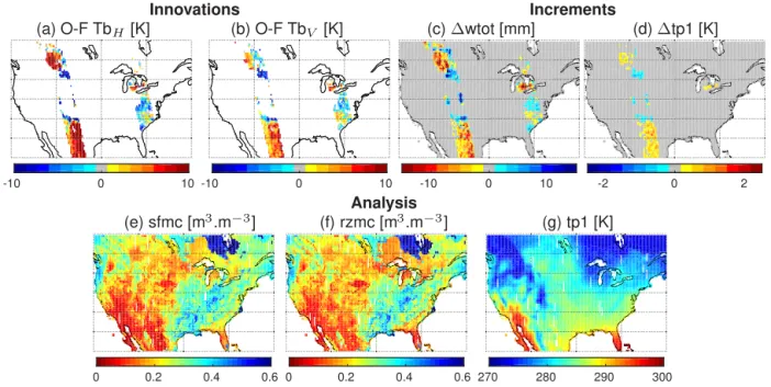
Figure 2.Soil moisture and temperature analysis on 30 April 2015 at 12:00 UTC for the Tb_fit assimilation system. (a,b) Tb innovations (O–F) at a 40◦incidence angle forH- andV-polarization respectively; (c,d) increments in total profile water (1wtot) and first soil layer temperature (1tp1), respectively; (e,f,g) assimilation analyses of surface soil moisture (sfmc), root-zone soil moisture (rzmc), and soil temperature (tp1), respectively.
quantity is easily understandable and thus simplifies the dis-cussion.
Figures 2 and 3 illustrate the concept for Tb assimila-tion and SM retrieval assimilaassimila-tion, respectively. Figure 2a–b show swaths of footprint-scale bias-corrected Tb_fit innova-tions (mapped onto the 36 km EASEv2 grid), forH- andV -polarization at a 40◦incidence angle from the single-angle Tb assimilation system. The Tb innovations are then trans-formed into soil moisture and temperature increments using Eq. (1). Where Tb innovations are warm, the soil water is re-duced and the temperature is increased. Figure 2c shows the total profile water increments1wtot and Fig. 2d shows incre-ments to the first soil layer temperature1tp1. Increments to the surface temperature prognostic variables (Sect. 2.3;1tc1, 1tc2,1tc4) are similar (not shown). Finally, the increments are added to the forecasted fields to create spatially complete analysis maps of surface and root-zone soil moisture, as well as surface temperature and soil temperature (Fig. 2e–g).
Similarly, Fig. 3a shows the SM innovations from the SM retrieval assimilation at the same time as in Fig. 2. Areas with positive (wet) SM innovations in the SM retrieval assimila-tion roughly correspond to negative (cold) Tb innovaassimila-tions in the Tb assimilation system (Fig. 2a–b). Note that the color bars for Tb and SM throughout the paper are chosen accord-ing to the rule of thumb that a 2–3 K change in Tb corre-sponds to a 0.01 m3m−3change in soil moisture, but keep in mind that the relationship between Tb and SM is nonlin-ear and varies with time, location, and incidence angle. Next, the SM innovations are converted to soil moisture increments
Innovations Increments
(a) O-F SM [m3.m−3] (b)∆wtot [mm]
-0.02 0 0.02 -10 0 10
Analysis
(c) sfmc [m3.m−3] (d) rzmc [m3.m−3]
0 0.2 0.4 0.6 0 0.2 0.4 0.6
(1wtot; Fig. 3b); no increment to surface or soil temperature is calculated. Figures 2c and 3b show that the Tb and SM retrieval assimilation systems produce wtot increments with somewhat different large-scale patterns, which is further dis-cussed in Sect. 4.2. Finally, Fig. 3c–d show the resulting sur-face and root-zone soil moisture analysis fields obtained by adding the increments to the model forecast fields. For both the Tb and SM retrieval assimilation systems, the analysis in-crements blend smoothly into the forecast fields; that is, the analysis maps do not reveal sharp spatial edges that would re-veal the geometry of the assimilated satellite swaths. Further details about this figure are discussed in Sect. 4.1.
3.2 Tb and SM innovation bias
To limit the long-term biases between Tb observations and simulations, the RTM was calibrated (Sect. 2.3). The 5-year average absolute bias between SMOS Tb and forecasted Tb is about 2 K across the domain. In general, slightly warm model biases are found in the boreal zones and cold model biases over the central part of the US (not shown), but larger seasonal Tb biases remain, primarily due to systematic er-rors in the modeled temperature and vegetation. The season-ally varying climatological Tb bias is removed prior to data assimilation for each angle, polarization, and overpass time separately, as described in De Lannoy and Reichle (2016). The Tb innovation biases are calculated over the period 1 July 2010–1 May 2015 for each individual 36 km grid cell without spatial sampling.
The CLSM soil moisture was not calibrated for lack of global observations that would support such an effort and because modeled soil moisture does not necessarily repre-sent soil moisture as observed in the field anyway (Koster et al., 2009). Unlike biases in Tb innovations, the biases in the SM innovations are more stationary and do not depend on seasonal temperature variations. Therefore, the SM inno-vation biases are not corrected seasonally, but instead cumu-lative distribution function (CDF) matching between the ob-servations and simulations is performed (Reichle and Koster, 2004) to reconcile the differences in long-term mean, vari-ance, and higher moments, as in earlier retrieval assimilation studies (Liu et al., 2011; Draper et al., 2012). The observed and simulated SM CDFs are computed for the entire study period, i.e., for 1 July 2010–1 May 2015, at each 36 km grid cell individually.
3.3 Random forecast and observation error
The imposed ensemble forecast perturbations for Tb and SM retrieval assimilation are identical to those of De Lannoy and Reichle (2016) and not repeated here. The total obser-vation error standard deviation for SMOS Tb_7ang is set to 6 K, which yields near-optimal assimilation diagnostics on average across the globe. However, the diagnostics are not necessarily near-optimal in individual regions (De Lannoy
and Reichle, 2016). The input observation error standard de-viation for SM retrievals is 0.04 m3m−3, in line with the soil moisture accuracy requirement for the recent SMOS and SMAP missions. The SM retrieval error standard deviation is rescaled following the CDF matching of the SM observa-tions and results in an effective mean error standard deviation of 0.02 m3m−3, with larger values in the wetter eastern part, which exhibits a higher temporal variability in soil moisture simulations, and lower values in the drier, western part of the study domain (not shown). In all cases, the spatial observa-tion error correlaobserva-tion length is 0.25◦. In the case of multi-angle Tb_7ang assimilation, interangular error correlations are imposed as in De Lannoy and Reichle (2016).
Observation errors in Tb data or SM retrievals are a com-bination of instrument error and representation error (Cohn, 1997; van Leeuwen, 2015). The 6 K Tb error consists of a ra-diometric error of about 4 K for individual incidence angles (instrument error) plus 4.5 K representation inaccuracies (in our system, i.e., based on the near-optimal 6 K observation error) due to errors in the RTM, the spatial aggregation, or other discrepancies between Tb observations and forecasts (6=p42+4.52). For Tb_fit observations, the instrument er-ror may be slightly reduced compared to that for Tb_7ang after the angular smoothing, but the representation error re-mains similar. SM observations contain retrieval errors due to errors in the RTM and in the input L1 Tb observations, as well as representation error due to, e.g., the inherently differ-ent nature of simulated and observed soil moisture (Koster et al., 2009). In either case, the representation error depends on the soil moisture and temperature dynamics and should ideally be modeled as a function of time and location, but we chose a constant input observation error standard deviation in this paper for simplicity. For SM retrieval assimilation, some spatial error variability is introduced after rescaling in line with the CDF matching.
3.4 Tb or SM retrieval assimilation
sys-tems is to an optimal calibration of its model and observation error parameters.
4 Results
4.1 Observation and forecast diagnostics 4.1.1 Number of assimilated observations
Let us revisit Figs. 2a–b and 3a to further highlight some differences between the various assimilated SMOS obser-vations. First, the swath width for Tb innovations is much narrower than that of the SM innovations because the as-similated Tb observations are strictly limited to the alias-free zone within the full swath, while the assimilated SM retrievals are retained in the extended alias-free zone. Fur-thermore, the swath width of the Tb_fit innovations is nar-rower than that of the multi-angle assimilation (not shown) because the fitting requires sufficient data at a range of in-cidence angles and lower angle data are not available at the outer edges of the swaths. Note that SMAP provides useable Tb measurements over a much wider swath (not shown).
The different swath widths result in different numbers of observation sets assimilated in each of the three experiments. Figure 4a–c show the average number of assimilated obser-vation sets (defined in Sect. 3.1) over the study period 1 July 2010–1 May 2015. The number of observation sets is small-est (one every 4 days) for Tb_fit and largsmall-est for SM retrievals (one every 2 days), because the swath width is narrowest for Tb_fit and widest for SM retrievals. The northern areas and the western mountain ranges have the fewest observations, because data are not used when the soil is frozen or snow cov-ered. Tb observations are not assimilated in many small areas scattered around the study domain, where more than 5 % of open water is found in the footprint, based on the underlying GEOS-5 land mask. For the SM retrievals, the screening for an excessive (>5 %) water fraction is only based on the prod-uct science flags, not on GEOS-5 information. Data gaps in the SM retrievals are found in the western mountain ranges and in the vegetated southeastern part of the US. The data coverage is also different for Tb and SM retrieval assimila-tion because the availability of the climatological informa-tion needed for the innovainforma-tion bias correcinforma-tion (Sect. 3.2) is different for the Tb and SM retrieval observations.
4.1.2 Actual observation and forecast errors
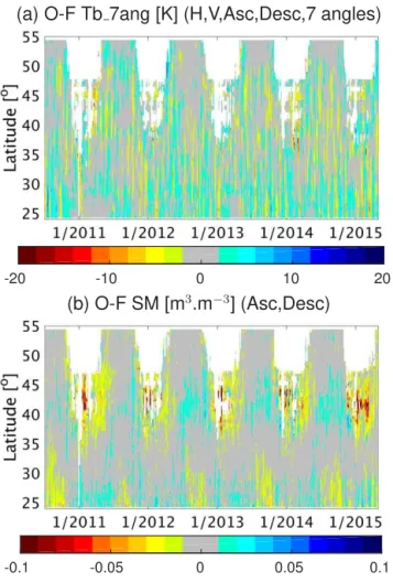
The long-term mean observation-minus-forecast differences (O–F, or innovations) are unbiased by design (Sect. 3.2). The Hovmüller plots for two data assimilation cases in Fig. 5 re-veal that the temporal pattern in area-averaged biases is fairly random for the Tb_7ang assimilation case (very similar for Tb_fit assimilation, not shown), whereas it shows a slight seasonal pattern in the SM retrieval assimilation case. This small difference is not surprising, given that the Tb
innova-tion bias is seasonally corrected, whereas the SM innovainnova-tion bias is not.
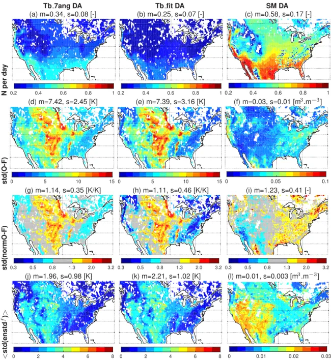
The time series standard deviation of the innovations, that is, the root-mean-square difference (RMSD) between SMOS observations and simulations, represents the total observation and forecast error that is present in the assimilation system (Desroziers et al., 2005). The spatial patterns of this diag-nostic are very different for Tb and SM retrieval assimila-tion. Figure 4d–e show values of about 7.4 K for Tb_7ang and Tb_fit, with larger values (exceeding 10 K) in the cen-tral plains and along the Mississippi, where agricultural prac-tices, such as altering crop rotation and irrigation, are ob-served by SMOS, whereas interannual variations in vege-tation are not simulated by the model or provided as input to the model. Along the eastern coast and in the southeast, the temporal standard deviation in the innovations is low (2– 3 K): forests show a limited interannual variability, and under dense vegetation Tb is only marginally sensitive to soil mois-ture and depends primarily on vegetation characteristics and (physical) temperature.
The standard deviation in the SM innovations in the SM re-trieval assimilation (Fig. 4f) is 0.03 m3m−3, showing larger values in the wetter vegetated east and smaller values in the drier west, with the exception of the western coast. Surpris-ingly, even though altering crop rotation and irrigation are not simulated, the values over the central agricultural area are not higher than elsewhere in the domain. This good agreement between SMOS SM retrievals and our simulations is partly due to the bounded nature of SM (unlike Tb) and the CDF matching between both.
Our current system has a Tb sensitivity to soil moisture of about 1.3 K/0.01 m3m−3 across the domain, averaged over all incidence angles and polarizations. A standard deviation in SM innovations of 0.03 m3m−3would thus roughly corre-spond to a standard deviation in Tb innovations of about 4 K, but instead we find 7.4 K across the study domain in the Tb assimilation systems. The Tb observations thus either have a comparably higher observation (including representation) er-ror or they contain more information than the SM retrievals. At this point, we anticipate that the larger Tb innovations in the central plains may indicate that the Tb observations con-tain more unfiltered information about soil moisture (e.g., ir-rigation) and that the Tb observation error is higher due to shortcomings, e.g., in the vegetation modeling (representa-tion error).
4.1.3 Actual vs. simulated observation and forecast errors
In a near-optimal filtering system, that is, a system that cor-rectly simulates the actual model and observation errors, the standard deviation of the normalized innovations[yκ,i−
ˆ y−κ,i]λ/
q
do-Tb 7ang DA Tb fit DA SM DA (a) m=0.34, s=0.08 [-] (b) m=0.25, s=0.07 [-] (c) m=0.58, s=0.17 [-]
N
per
da
y
0.2 0.4 0.6 0.8 1 0.2 0.4 0.6 0.8 10.2 0.4 0.6 0.8 1
(d) m=7.42, s=2.45 [K] (e) m=7.39, s=3.16 [K] (f) m=0.03, s=0.01 [m3 .m−3]
std(O-F) 0 5 10 15 0 5 10 15 0 0.05 0.1
(g) m=1.14, s=0.35 [K/K] (h) m=1.11, s=0.46 [K/K] (i) m=1.23, s=0.41 [-]
std(normO-F) 0.3 0.5 0.8 1.3 2.0 3.2 0.3 0.5 0.8 1.3 2.0 3.2 0.3 0.5 0.8 1.3 2.0 3.2 (j) m=1.96, s=0.98 [K] (k) m=2.21, s=1.02 [K] (l) m=0.01, s=0.003 [m3
.m−3]
<
std(enstd
f)
>
0 2 4 6 8 0 2 4 6 8 0 0.01 0.02 0.03
Figure 4.Observation-space assimilation diagnostics for the period from 1 July 2010 to 1 May 2015. Number of assimilated observation sets for(a)Tb_7ang assimilation,(b)Tb_fit assimilation, and(c)SM retrieval assimilation. Standard deviation of the(d)Tb innovations from Tb_7ang assimilation,(e)Tb innovations from Tb_fit assimilation, and(f)SM innovations from SM retrieval assimilation. (g,h,i) Same as (d,e,f), but for normalized innovations (normO–F). Ensemble standard deviation of the (j) Tb forecast error for Tb_7ang assimilation,
(k)Tb forecast error for Tb_fit assimilation, and(l)surface soil moisture forecast error for SM retrieval assimilation. The titles show the spatial mean (m) and standard deviation (s) across each map.
main (and across all angles and polarizations for Tb assim-ilation), this metric is 1.14, 1.11, and 1.23 (–) for Tb_7ang, Tb_fit, and SM retrieval assimilation, respectively. The fig-ure thus suggests that, on average, the simulated errors in the assimilation system only slightly underestimate the ac-tual errors. But the figures also show that the metric varies strongly across the domain and exhibits very different spatial patterns for Tb and SM retrieval assimilation. For Tb_7ang
(a) O-F Tb 7ang [K] (H,V,Asc,Desc,7 angles)
-20 -10 0 10 20
(b) O-F SM [m
3.m
−3] (Asc,Desc)
-0.1 -0.05 0 0.05 0.1
Figure 5.Hovmüller plots showing the temporal evolution of lon-gitudinally averaged innovations (O–F) for the period from 1 July 2010 to 1 May 2015.(a)Tb_7ang innovations, averaged overH -and V-polarization, ascending and descending swaths, and over seven incidence angles.(b)SM innovations, averaged over ascend-ing and descendascend-ing swaths.
only marginally sensitive to soil moisture uncertainties under dense vegetation. For SM retrieval assimilation, the pattern is reversed, with the largest values in the eastern half of the do-main, suggesting that here the simulated errors underestimate the actual errors. Values less than 1 are found in most of the western half of the domain, where the SM retrieval assimila-tion seems to overestimate the actual errors.
To further interpret the actual and simulated error magni-tudes, Fig. 4j–k show the ensemble spread in the Tb fore-casts (that is, the simulated forecast error standard deviation)
q
[Cov(yˆ−κ,i,yˆ−κ,i)]λλ. Averaged across all angles and
polar-izations λ, the values are around 2 K when averaged across the entire domain. Larger values (3 K) are found in the cen-tral and dry western part, and smaller values (1 K) in the wet-ter easwet-tern part. This patwet-tern is similar for the SM ensemble spread in the SM retrieval assimilation system (Fig. 4l). In dry climates, the root-zone soil moisture often drops to the
wilting point, remains stagnant and no longer replenishes the surface. This results in increased sensitivity of the surface soil moisture to perturbations in meteorological conditions, and thus in higher uncertainty estimates for surface soil mois-ture in dry climates.
Given that the Tb observation errorp[Rκ,i]λλis set to 6 K for each individual angle, polarization, and overpass time in the Tb assimilation, the approximate total assigned ob-servation and forecast error is 6.1 K (√62+22) across the study domain, 6.7 K (√62+32) in the central area, and 6 K (√62+12) in the eastern Appalachian area. Because the as-signed observation error is uniformly set to 6 K, the spatial variability in the total simulated errors is thus too small com-pared to the actual errors (Fig. 4d–e), which ranges from more than 10 K in the central area to around 2–3 K in the eastern Appalachian area.
The SM observation error (after rescaling) is 0.02 m3m−3 on average across the domain, with higher values in the east-ern part and lower values in the westeast-ern part, with the ex-ception of Mexico, California, and western Oregon, where higher observation errors are found (Sect. 3.3). This general pattern is reversed in the SM forecast errors. Combined, the spatial variability in the SM observation and forecast errors does not capture the spatial variability in the actual errors (Fig. 4f), which leads to an overestimation of the errors in the west and an underestimation in the east.
4.2 Analysis increments 4.2.1 Spatio-temporal patterns
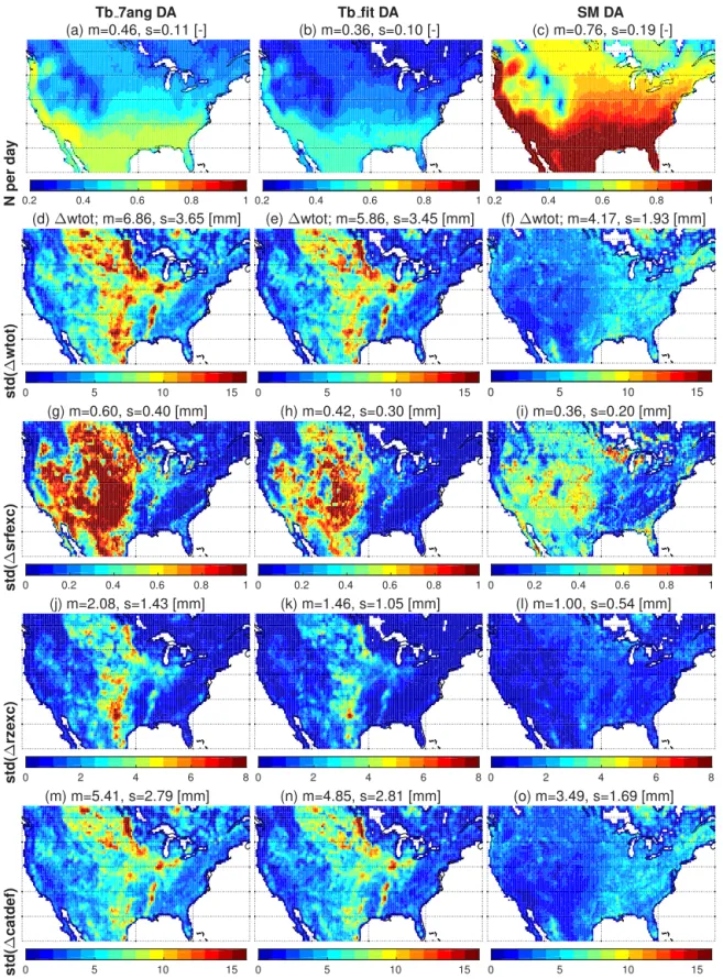
The Kalman filter translates footprint-scale innovations into 36 km increments. Because of the spatially distributed (3-D) filtering (Sect. 3.1), the number of increments in Fig. 6a– c is about 1.4 times the number of assimilated observation sets (Fig. 4a–c). Many areas with missing observations (or observation predictions) are filled through interpolation and extrapolation. With SM retrieval assimilation, there is almost one increment per day.
Figure 6d–f show the temporal standard devia-tions in the increments for the total soil profile water (1wtot=1srfexc+1rzexc–1catdef). The area average (±standard deviation) values are 6.9±3.7 mm for Tb_7ang assimilation, 5.9±3.5 mm for Tb_fit assimilation, and 4.2±1.9 for SM retrieval assimilation. After scaling for the (variable) profile depth, the area-average values in volumet-ric soil moisture units are 3.4±1.7×10⁻³ for Tb_7ang assimilation, 2.9±1.7×10⁻³ for Tb_fit assimilation, and 2.3±1.9×10⁻³m3m−3for SM retrieval assimilation.
stan-Tb 7ang DA Tb fit DA SM DA
(a) m=0.46, s=0.11 [-] (b) m=0.36, s=0.10 [-] (c) m=0.76, s=0.19 [-]
N
per
da
y
0.2 0.4 0.6 0.8 1 0.2 0.4 0.6 0.8 1 0.2 0.4 0.6 0.8 1
(d)∆wtot; m=6.86, s=3.65 [mm] (e)∆wtot; m=5.86, s=3.45 [mm] (f)∆wtot; m=4.17, s=1.93 [mm]
std(
∆
wtot)
0 5 10 15 0 5 10 15 0 5 10 15
(g) m=0.60, s=0.40 [mm] (h) m=0.42, s=0.30 [mm] (i) m=0.36, s=0.20 [mm]
std(
∆
srf
e
xc)
0 0.2 0.4 0.6 0.8 1 0 0.2 0.4 0.6 0.8 1 0 0.2 0.4 0.6 0.8 1
(j) m=2.08, s=1.43 [mm] (k) m=1.46, s=1.05 [mm] (l) m=1.00, s=0.54 [mm]
std(
∆
rz
e
xc)
0 2 4 6 8 0 2 4 6 8 0 2 4 6 8
(m) m=5.41, s=2.79 [mm] (n) m=4.85, s=2.81 [mm] (o) m=3.49, s=1.69 [mm]
std(
∆
catdef)
0 5 10 15 0 5 10 15 0 5 10 15
Figure 6. Statistics of the increments, calculated for the period from 1 July 2010 to 1 May 2015. Number of increments per day for
dard deviations (Fig. 4d–f), which are very different for Tb and SM retrieval assimilation. The catdef increments pertain to the entire profile depth (which typically ranges between 2 and 3 m) and they presumably have a relatively small im-pact on the upper 5 cm soil layer (surface soil moisture): the domain-averaged magnitude of 5.4, 4.9, and 3.5 mm for catdef increments due to Tb_7ang, Tb_fit or SM retrieval assimilation, respectively (Fig. 6m–o), would linearly scale to about 0.1 mm for a 5 cm soil layer. This is a rough ap-proximation: in reality the part of catdef that contributes to the 5 cm soil moisture cannot be calculated without com-puting the entire balanced profile. However, the approximate 0.1 mm is considerably less than the 0.6, 0.4, and 0.4 mm for the corresponding srfexc increments (Fig. 6g–i), which are directly applied to the upper 5 cm soil layer. The increments in rzexc (Fig. 6j–l) are relatively the smallest, because this variable is not perturbed by design.
Both Tb and SM retrieval assimilation show similar spa-tial patterns in the standard deviations of srfexc increments (Fig. 6g–i): the largest increments are found in the dry west and the smallest in the wetter east. The patterns in srfexc in-crements agree with the patterns in the ensemble forecast un-certainty for this variable (not shown, but implied by the Tb and soil moisture uncertainty in Fig. 4j–l). The srfexc val-ues are small with small uncertainties, and the increments are thus similarly bounded in both Tb and SM retrieval as-similation, yielding comparable spatial increment patterns.
Finally, Fig. 7 compares spatially and temporally col-located wtot, srfexc, and rzexc increments obtained with Tb_7ang assimilation, Tb_fit assimilation, and SM retrieval assimilation; i.e., the figure shows all pairs of increments available from two assimilation cases. The scatter plots show that the increments are usually small and unbiased. The cor-relation between the wtot increments (Fig. 7a) obtained by Tb_7ang and Tb_fit assimilation is 0.7, and aligns with the expectation that either Tb assimilation experiment roughly corrects for the same events. In contrast, the correlation between the increments obtained by Tb_7ang and SM re-trieval assimilation is only 0.3 (Fig. 7b). The figure is sim-ilar when comparing the Tb_fit and SM retrieval assimila-tion (not shown). For srfexc and rzexc (Fig. 7c–f), the incre-ments are again similar for Tb_7ang and Tb_fit assimilation, but different for Tb and SM retrieval assimilation. For all soil moisture prognostic variables, Tb assimilation leads to larger increments than SM retrieval assimilation. The different as-similation systems thus introduce distinct corrections to the modeled soil moisture trajectories.
4.2.2 Discussion
In a nutshell, Eq. (1) states that the increments are given by the product of the Kalman gain and the innovations. To ex-plain the differences in increment patterns between Tb and SM retrieval assimilation, we must therefore consider each system’s innovations and Kalman gains. The relatively larger
∆wtot [mm]
(a) R=0.72 (b) R=0.33
-50 0 50
Tb_7ang DA
-50 0 50
Tb_fit DA
-50 0 50
Tb_7ang DA
-50 0 50
SM DA
1
102
104
∆srfexc [mm]
(c) R=0.81 (d) R=0.41
-5 0 5
Tb_7ang DA
-5 0 5
Tb_fit DA
-5 0 5
Tb_7ang DA
-5 0 5
SM DA
1
102
104
∆rzexc [mm]
(e) R=0.77 (f) R=0.33
-20 0 20
Tb_7ang DA
-20 0 20
Tb_fit DA
-20 0 20
Tb_7ang DA
-20 0 20
SM DA
1
102
104
Figure 7.Spatially and temporally collocated analysis increments from (a,c,e) Tb_fit assimilation and (b,d,f) SM retrieval assim-ilation vs. the same from Tb_7ang assimassim-ilation for (a,b) profile-integrated wtot increments, (c,d) srfexc increments, and (e–f) rzexc increments. Increments are from the period 1 July 2010 to 1 May 2015. The plot range is limited to the maximum value of 10 times the standard deviation in either experiment, and divided into 100 even sample bins. Colors indicate the number of sample points within each 1.5, 0.13, or 0.44 mm bin for 1wtot, 1srfexc, and 1rzexc, respectively.R is the spatio-temporal Pearson correlation coefficient between the individual increments from two assimilation experiments.
magnitude of the Tb innovations compared to the SM inno-vations (Sect. 4.1.2) contributes to the fact that the Tb assim-ilation results in larger soil moisture increments. This is the case even though the SM retrieval assimilation (unlike Tb as-similation) applies increments only to moisture variables and does not adjust modeled temperatures.
notresponsible for the larger wtot increments in the central grass and crop areas, because these areas exhibit low values for the microwave roughness parameter (h <0.2, not shown) and a high sensitivity of Tb to soil moisture (as confirmed by the high forecast Tb errors in Fig. 4j–k). That is, in these ar-eas commensurately large Tb innovations (O–F) values result in only small updates to soil moisture.
Second, the choice of a spatially uniform observation er-ror covariance in the Tb assimilation experiment creates an imprint of the innovation pattern in the increment pattern. Higher increments are found in the agricultural areas with large Tb innovation standard deviations (Fig. 4d–e), because irrigation is not modeled and vegetation is not accurately pa-rameterized. Since the filter is not set up to correct the latter, occasional excessive increments to soil moisture and temper-ature may be introduced. Such shortcomings could be miti-gated by a more sophisticated assignment of Tb observation (representation) errors.
For SM retrieval assimilation, the pattern of the SM in-novation standard deviation (RMSD) is similarly visible in the increments, with smaller values in the west and higher values in the east. Here again, the true spatio-temporal na-ture of the observation errors is not capna-tured in the assigned observation error covariance and therefore propagated into the increments. Note also that the 0.03 m3m−3 SM inno-vation standard deviation (top 5 cm, Fig. 4f) is translated into a standard deviation of profile moisture increments of 0.002 m3m−3(Fig. 6f rescaled by profile depth), but these increments are not equally distributed; i.e., larger increments are found for surface soil moisture and smaller increments for the deeper profile.
4.3 In situ validation
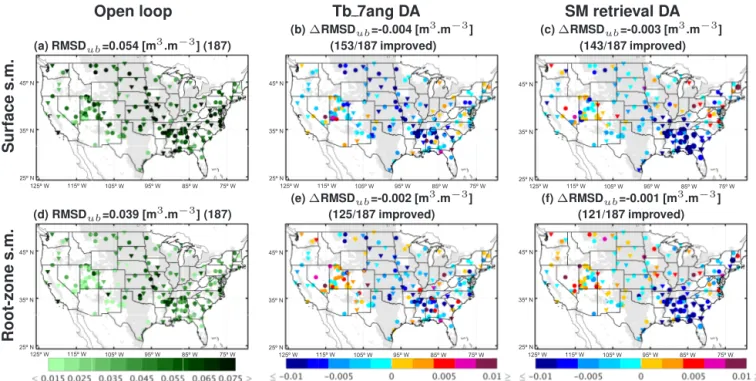
The above discussion highlights similarities and stark con-trasts in how the Tb and SM retrieval assimilation systems operate. In this section, we look at the effect of these dif-ferences on the skill of the assimilation estimates vs. in situ observations. Figure 8 shows the RMSDub(Sect. 2.4) for the model-only open-loop (OL) simulation, and the change in RMSDub (Sect. 2.4) between the OL simulation and either the Tb_7ang or SM retrieval data assimilation (DA) experi-ment (1RMSDub=RMSDub(DA) – RMSDub(OL)) at indi-vidual SCAN and USCRN sites, for the period 1 July 2010– 1 May 2015. The gray background shading indicates areas with modest topographic complexity and vegetation cover and where the satellite observations are most sensitive to surface soil moisture (details in De Lannoy and Reichle, 2016). The OL simulation has an average RMSDubvalue of 0.054 m3m−3for surface soil moisture and 0.039 m3m−3for root-zone soil moisture. Looking more closely, the RMSDub values are generally higher in the central and wetter eastern regions. In dry areas, the RMSDub is limited, because the time series show a limited variability for lack of much precip-itation. On average, both assimilation experiments introduce
improvements at about 80 % of the sites for surface soil mois-ture, with spatially averaged1RMSDub values of −0.004 and−0.003 m3m−3for Tb_7ang and SM retrieval assimila-tion, respectively. (Spatial average metrics are computed us-ing a cluster-based algorithm, Sect. 2.4.) The improvements are also propagated to the root-zone soil moisture (65 % of sites improved) with smaller average1RMSDub values of
−0.002 and−0.001 m3m−3, respectively.
The domain-average1RMSDub values caused by assim-ilation are only barely statistically significant for surface soil moisture in “favorable” areas, i.e., where the satellite observations are most sensitive to soil moisture (indicated with green background shading in Fig. 8). The differences between Tb_7ang, Tb_fit, or SM retrieval assimilation are not significant. The assimilation contributes an average rela-tive improvement in surface soil moisture of 7 % of the OL RMSDubin favorable locations and 4 % in non-favorable ar-eas. Both Tb and SM retrieval assimilation show improve-ments in the central and eastern parts of the US, but per-form poorly in the western dry mountain areas, where the RMSDubfor the OL was small and the assimilation may have introduced some additional noise. The Tb_7ang assimilation shows the largest improvements in the central US, whereas the SM retrieval assimilation shows the largest improvements in the southeastern part, for both surface and root-zone soil moisture. It is possible that the Tb assimilation has a larger impact in the central US than the SM retrieval assimilation, because irrigation events may be filtered in the SM retrievals (and perhaps partly assigned to vegetation opacity retrievals). The bar plots in Fig. 9 summarize the average anomR val-ues for the open-loop and data assimilation experiments, af-ter stratifying all SCAN and USCRN sites into “favorable” and “non-favorable” categories (gray vs. white background in Fig. 8). The figures show that the open-loop anomR val-ues for surface soil moisture are similar for both the favor-able and non-favorfavor-able areas (0.51 and 0.50, respectively). However, data assimilation has a larger impact in favor-able areas, where all assimilation schemes introduce sig-nificant improvements (anomR=0.63, 0.61, and 0.59 for Tb_7ang, Tb_fit, and SM retrieval assimilation). In non-favorable areas, the improvements are smaller but still sig-nificant (anomR=0.57, 0.56, and 0.54, for Tb_7ang, Tb_fit, and SM retrieval assimilation).
Open loop Tb 7ang DA SM retrieval DA (b)∆RMSDub=-0.004 [m3.m−3] (c)∆RMSDub=-0.003 [m3.m−3] (a) RMSDub=0.054 [m3.m−3] (187) (153/187 improved) (143/187 improved)
S
u
rf
a
c
e
s
.m
.
(e)∆RMSDub=-0.002 [m3.m−3] (f)∆RMSDub=-0.001 [m3.m−3] (d) RMSDub=0.039 [m3.m−3] (187) (125/187 improved) (121/187 improved)
R
o
o
t-z
o
n
e
s
.m
.
45º N
35º N
25º N
45º N
35º N
25º N
45º N
35º N
25º N
45º N
35º N
25º N
125º W 115º W 105º W 95º W 85º W 75º W 125º W 115º W 105º W 95º W 85º W 75º W
125º W 115º W 105º W 95º W 85º W 75º W
125º W 115º W 105º W 95º W 85º W 75º W 45º N
35º N
25º N
45º N
35º N
25º N
125º W 115º W 105º W 95º W 85º W 75º W 125º W 115º W 105º W 95º W 85º W 75º W
Figure 8.Unbiased RMSD (RMSDub) for the model-only open-loop (OL) simulation, and change in unbiased RMSD (1RMSDub) due to data assimilation at (circles) SCAN and (triangles) USCRN sites for (a,b,c) surface and (d,e,f) root-zone soil moisture. The skill of (a,d) the open-loop simulation is the reference value for the changes in skill due to (b,e) Tb_7ang and (c,f) SM retrieval assimilation. Statistically significant changes are marked by larger symbols (e.g., the southeastern US for SM retrieval assimilation). Metrics are calculated across 3 h time steps during the period from 1 July 2010 to 1 May 2015. The titles indicate the spatial mean (1)RMSDubacross all sites with clustering (31 clusters). The gray background shading marks areas with limited vegetation and topographic complexity based on model parameters.
Overall, the skill metrics are comparable for the Tb_7ang and Tb_fit assimilation (Fig. 9). The results from SM re-trieval assimilation are slightly worse than those from Tb as-similation, which may indicate that Tb observations indeed still contain more information (Sect. 4.2) than the SM re-trievals, which are implicitly filtered during the retrieval pro-cess. However, the differences between the domain-averaged skill values of the various assimilation schemes are minimal. Furthermore, when running the assimilation scheme with dif-ferent spatially constant Tb observation error parameters, the skill metrics only changed marginally. This shows that our skill metrics are relatively insensitive to uniform changes in the data assimilation parameters. One reason for this is that the skill metrics are presented as (clustered) spatial averages, which compensate for large local differences. It is expected that the skill of our data assimilation systems can only be fur-ther improved by using a more localized (in space and time) approach to optimizing the assimilated observations (e.g., L2 SM retrievals) and the forecast and observation error param-eters in the EnKF.
Finally, unlike Liu et al. (2011), the skill improvements in this study are smaller when we correct the re-analysis precipitation input with gauge-based precipitation data (Re-ichle and Liu, 2014). This and other recent improvements in the GEOS-5 modeling system make it increasingly
chal-lenging to obtain significant skill improvements from the as-similation of microwave observations over areas for which high-quality forcing data are available, such as the domain studied here. The benefits of the microwave-based soil mois-ture assimilation system are expected to be greater in areas with poorer ancillary inputs to the modeling system. This as-pect will be further investigated through the validation of the global SMAP L4_SM data product.
5 Conclusions
(a) Surface soil moisture
Favorable Non-favorable 0.4
0.5 0.6
anomR [-] N=98(24) N=83(22)
(b) Root-zone soil moisture
Favorable Non-favorable 0.4
0.5 0.6
anomR [-] N=98(24) N=83(22)
Open loop,
Tb 7ang DA,Tb fit DA,SM DA
Figure 9.Performance of open-loop and data assimilation experi-ments in terms of anomaly correlations (anomR) calculated across 3 h analyses and forecast time steps from 1 July 2010 to 1 May 2015 for(a)surface and(b)root-zone soil moisture. The bars show skill metrics averaged over sites in either favorable or non-favorable ar-eas, where favorable areas refer to the areas indicated by the gray background shading in Fig. 8. The variableN is the total number of SCAN and USCRN sites considered for each category, with the number of clusters in parentheses. The error bars reflect cluster-averaged 95 % confidence intervals.
the assimilated retrievals and careful selection of the ancil-lary data, SM retrieval assimilation may become a coequal alternative.
Three different data products from the SMOS mission are assimilated separately into the GEOS-5 land surface model to improve estimates of surface and root-zone soil moisture and to study the workings of each assimilation system. The first product consists of L1-based data of multi-angle, dual-polarization Tb observations at the bottom of the atmosphere. The second product is a derived 40◦Tb product that mim-ics SMAP data. The third product is the operational L2 SM dataset. Special care is taken during quality control and pro-cessing of the satellite observations prior to assimilation and within the assimilation system. The Tb assimilation uses a distributed EnKF with a temporally variable Tb bias mitiga-tion, a system that is also used for the SMAP L4_SM product (Reichle et al., 2016). The SM retrieval assimilation uses a similar system, but with CDF matching instead to eliminate the more stationary SM innovation biases. The study covers most of North America for the period of 1 July 2010–1 May 2015.
The Tb and SM innovations show very different spatial patterns and the number of assimilated observations differs because of different needs for data screening and bias mitiga-tion. Based on the average sensitivity of Tb to soil moisture, the magnitude of the Tb innovations is comparably larger than that of the SM innovations, which may either
intro-duce more information or more error into the Tb assimilation system. The Tb and SM retrieval assimilation schemes also yield surprisingly different spatio-temporal increment pat-terns, leading to very different adjustments to the modeled soil moisture trajectories. Despite these stark differences, the various assimilation schemes yield soil moisture estimates with similar average skill metrics, computed from a set of 187 SCAN and USCRN sites across the US. Compared to in situ observations, both Tb and SM retrieval assimilations yield anomaly correlations around or larger than 0.6 for both the surface and root-zone soil moisture in “favorable” ar-eas, where the satellite data are expected to better represent the soil moisture conditions, i.e., in areas with limited topo-graphic complexity and limited vegetation. The anomaly cor-relation with data assimilation is between 0.5 and 0.6 in non-favorable areas. The data assimilation introduces significant improvements over the model-only simulations for surface soil moisture everywhere, but the improvements are much larger in favorable areas. For the root zone, improvements are also found, but without statistical significance. While no sig-nificant differences in domain-averaged skills can be found between the various assimilation systems, there are large lo-cal differences in performance between the Tb and SM re-trieval assimilation which may be due to differences in infor-mation content and screening of the observations, and differ-ences in how close each of the systems is to an optimal cali-bration of its model and observation error parameters. There-fore, we expect that soil moisture data assimilation systems can be further improved only if the systems manage to bet-ter simulate the spatial and temporal variations of the actual errors in the model and the observations. Furthermore, the SM retrieval assimilation results will benefit from any future improvement in the SM retrievals.
In line with our findings for the SMOS data assimilation, we anticipate that future versions of the Tb assimilation sys-tem for the SMAP L4_SM product may benefit from an im-proved characterization of spatial model and observation er-ror structures, and from a better representation of some mod-eling components, such as, e.g., vegetation. In addition, given that SMOS and SMAP both provide L-band Tb observations, future assimilation systems should consider a joint assimila-tion of SMOS and SMAP Tb data. In such a system, it is important to consider the different instrument, Tb process-ing, and Tb error characteristics of the two L-band missions (De Lannoy et al., 2015).
6 Data availability
Acknowledgements. The NASA Soil Moisture Active Passive (SMAP) mission supported this study. The NASA Center for Climate Simulation (NCCS) at the Goddard Space Flight Center provided computational resources through the NASA High-End Computing (HEC) program. The authors thank the editors and reviewers for their input.
Edited by: B. Su
Reviewed by: Y. Zeng and two anonymous referees
References
Al-Yaari, A., Wigneron, J.-P., Ducharne, A., Kerr, Y., Wagner, W., Lannoy, G. D., Reichle, R., Bitar, A. A., Dorigo, W., Richaume, P., and Mialon, A.: Global-scale comparison of passive (SMOS) and active (ASCAT) satellite based microwave soil moisture re-trievals with soil moisture simulations (MERRA-Land), Remote Sens. Environ., 152, 614–626, 2014.
Alvarez-Garreton, C., Ryu, D., Western, A. W., Su, C.-H., Crow, W. T., Robertson, D. E., and Leahy, C.: Improving operational flood ensemble prediction by the assimilation of satellite soil moisture: comparison between lumped and semi-distributed schemes, Hy-drol. Earth Syst. Sci., 19, 1659–1676, doi:10.5194/hess-19-1659-2015, 2015.
Bell, J., Palecki, M., Baker, C., Collins, W., Lawrimore, J., Leeper, R., Hall, M., Kochendorfer, J., Meyer, T., Wilson, T., and Dia-mond, H.: US climate reference network soil moisture and tem-perature observations, J. Hydrometeorol., 14, 977–988, 2013. Bosilovich, M. G., Akella, S., Coy, L., Cullather, R., Draper, C.,
Gelaro, R., Kovach, R., Liu, Q., Molod, A., Norris, P., Wargan, K., Chao, W., Reichle, R., Takacs, L., Vikhliaev, Y., Bloom, S., Collow, A., Firth, S., Labow, G., Partyka, G., Pawson, S., Reale, O., Schubert, S. D., and Suarez, M.: MERRA-2: Initial Evalua-tion of the Climate, Tech. rep., NaEvalua-tional Aeronautics and Space Administration, Goddard Space Flight Center, Greenbelt, Mary-land, USA, 2015.
Brodzik, M. J., Billingsley, B., Haran, T., Raup, B., and Savoie, M.: Correction: Incremental but Significant Improvements for Earth-Gridded Data Sets, ISPRS Int. J. Geo.-Inf., 3, 1154–1156, 2014. Chakrabart, S., Bongiovanni, T., Judge, J., Zotarelli, L., and Bayer, C.: Assimilation of SMOS Soil Moisture for Quantifying Drought Impacts on Crop Yield in Agricultural Regions, IEEE J. Sel. Top. Appl., 7, 3867–3879, 2014.
Cohn, S.: An Introduction to Estimation Theory, J. Meteorol. Soc. Jpn., 75, 257–288, 1997.
De Lannoy, G. and Reichle, R.: Global Assimilation of Multi-Angle and Multi-Polarization SMOS Brightness Temperature Observa-tions into the GEOS-5 Catchment Land Surface Model for Soil Moisture Estimation, J. Hydrometeorol., 17, 669–691, 2016. De Lannoy, G., Reichle, R., and Pauwels, V.: Global Calibration of
the GEOS-5 L-band Microwave Radiative Transfer Model over Non-Frozen Land Using SMOS Observations, J. Hydrometeo-rol., 14, 765–785, doi:10.1175/JHM-D-12-092.1, 2013. De Lannoy, G., Koster, R., Reichle, R., Mahanama, S., and Liu, Q.:
An Updated Treatment of Soil Texture and Associated Hydraulic Properties in a Global Land Modeling System, J. Adv. Model. Earth Syst., 6, 23, doi:10.1002/2014MS000330, 2014a.
De Lannoy, G., Reichle, R., and Vrugt, J.: Uncertainty Quantifi-cation of GEOS-5 L-Band Radiative Transfer Model Parame-ters using Bayesian Inference and SMOS Observations, Remote Sens. Environ., 148, 146–157, doi:10.1016/j.rse.2014.03.030, 2014b.
De Lannoy, G., Reichle, R., Peng, J., Kerr, Y., Castro, R., Kim, E., and Liu, Q.: Converting Between SMOS and SMAP Level-1 Brightness Temperature Observations Over Nonfrozen Land, IEEE Geosci. Remote Sens. Lett., 12, 1908–1912, 2015. Desroziers, G., Berra, L., Chapnik, B., and Poli, P.: Diagnosis of
ob-servation, background and analysis-error statistics in observation space, Q. J. Roy. Meteorol. Soc., 131, 3385–3396, 2005. Diamond, H., Karl, T., Palecki, M., Bell, J., Leeper, R.,
Easter-ling, D., Lawrimore, J., Meyers, T., Helfert, M., Goodge, G., and Thorne, P.: US climate reference network after one decade of op-erations: status and assessment, BAMS, 94, 485–498, 2013. Draper, C. S., Reichle, R. H., Lannoy, G. J. M. D., and
Liu, Q.: Assimilation of passive and active microwave soil moisture retrievals, Geophys. Res. Lett., 39, L04401, doi:10.1029/2011GL050655, 2012.
Ducharne, A., Koster, R., Suarez, M., Stieglitz, M., and Kumar, P.: A catchment- based approach to modeling land surface processes in a GCM, Part 2, Parameter estimation and model demonstra-tion, J. Geophys. Res., 105, 24823–24838, 2000.
Entekhabi, D., Reichle, R. H., Koster, R. D., and Crow, W. T.: Per-formance Metrics for Soil Moisture Retrievals and Application Requirements, J. Hydrometeorol., 11, 832–840, 2010.
Entekhabi, D., Yueh, S., O’Neill, P., and Kellogg, K.: SMAP Hand-book, JPL Pasadena, CA, USA, 400–1567, 2014.
Fascetti, F., Pierdicca, N., Crapolicchio, L. P. R., and Munoz-Sabater, J.: A comparison of ASCAT and SMOS soil moisture retrievals over Europe and Northern Africa from 2010 to 2013, Int. J. Appl. Earth Obs., 45, 135–142, 2016.
Ford, T. W., Harris, E., and Quiring, S. M.: Estimating root zone soil moisture using near-surface observations from SMOS, Hy-drol. Earth Syst. Sci., 18, 139–154, doi:10.5194/hess-18-139-2014, 2014.
Kerr, Y., Waldteufel, P., Wigneron, J.-P., Delwart, S., Cabot, F., Boutin, J., Escorihuela, M.-J., Font, J., Reul, N., Gruhier, C., Juglea, S., Drinkwater, M., Hahne, A., Martin-Neira, M., and Mecklenburg, S.: The SMOS Mission: New Tool for Monitoring Key Elements of the Global Water Cycle, P. IEEE, 98, 666–687, 2010.
Kornelsen, K. C., Davison, B., and Coulibaly, P.: Application of SMOS Soil Moisture and Brightness Temperature at High Reso-lution With a Bias Correction Operator, IEEE JSTAR, 9, 1590– 1605, 2016.
Koster, R., Guo, Z., Yang, R., Dirmeyer, P., Mitchell, K., and Puma, M.: On the Nature of Soil Moisture in Land Surface Models, J. Climate, 22, 4322–4335, 2009.
Koster, R., Brocca, L., Crow, W., Burgin, M., and De Lan-noy, G.: Precipitation Estimation Using L-Band and C-Band Soil Moisture Retrievals, Water Resour. Res., 52, 7213–7225, doi:10.1002/2016WR019024, 2016.
Lievens, H., Tomer, S., Bitar, A. A., De Lannoy, G., Drusch, M., Dumedah, G., Hendricks-Franssens, H.-J., Kerr, Y., Pan, M., Roundy, J., Vereecken, H., Walker, J., Wood, E., Verhoest, N., and Pauwels, V.: SMOS soil moisture assimilation for improved stream flow simulation in the Murray Darling Basin, Australia, Remote Sens. Environ., 168, 146–162, 2015.
Liu, Q., Reichle, R. H., Bindlish, R., Cosh, M. H., Crow, W. T., de Jeu, R., Huffman, G., De Lannoy, G. J. M., and Jackson, T.: The contributions of precipitation and soil moisture observations to the skill of soil moisture estimates in a land data assimilation system, J. Hydrometeorol., 12, 750–765, 2011.
Mahanama, S. P., Koster, R., Walker, G., Tackacs, L., Reichle, R., Lannoy, G. D., Liu, Q., Zhao, B., and Suarez, M.: Land Boundary Conditions for the Goddard Earth Observing System Model Ver-sion 5 (GEOS-5) Climate Modeling System – Recent Updates and Data File Descriptions, Tech. rep., National Aeronautics and Space Administration, Goddard Space Flight Center, Greenbelt, Maryland, USA, 2015.
Munoz-Sabater, J., de Rosnay, P., Jiminnez, C., Isaksen, L., and Al-bergel, C.: SMOS Brightness Temperature Angular Noise: Char-acterization, Filtering, and Validation, IEEE T. Geosci. Remote Sens., 52, 5827–5839, 2014.
Piles, M., Sanchez, N., Vall-llossera, M., Camps, A., Martinez-Fernandez, J., Martinez, J., and Gonzaliez-Gambau, V.: A Down-scaling Approach for SMOS Land Observations: Evaluation of High-Resolution Soil Moisture Maps Over the Iberian Peninsula, IEEE JSTAR, 7, 3845–3857, 2014.
Reichle, R. H. and Koster, R.: Assessing the impact of horizontal er-ror correlations in background fields on soil moisture estimation, J. Hydrometeorol., 4, 1229–1242, 2003.
Reichle, R. H. and Koster, R.: Bias reduction in short records of satellite soil moisture, Geophys. Res. Lett., 31, L19501, doi:10.1029/2004GL020938, 2004.
Reichle, R. H. and Liu, Q.: Observation-Corrected Precipitation Es-timates in GEOS-5, Tech. rep., National Aeronautics and Space Administration, Goddard Space Flight Center, Greenbelt, Mary-land, USA, 2014.
Reichle, R. H., Walker, J. P., Houser, P. R., and Koster, R. D.: Ex-tended vs. Ensemble Kalman filtering for land data assimilation, J. Hydrometeorol., 3, 728–740, 2002.
Reichle, R. H., Lucchesi, R. A., Ardizzone, J., Kim, G.-K., Smith, E., and Weiss, B.: Soil Moisture Active Passive (SMAP) Mission Level 4 Surface and Root Zone Soil Moisture (L4_SM) Prod-uct Specification Document, Tech. rep., NASA Goddard Space Flight Center, GMAO Office Note No. 10 (Version 1.4), 2015. Reichle, R. H., De Lannoy, G. J. M., Liu, Q., Ardizzone, J., Chen,
F., Colliander, A., Conaty, A., Crow, W., Jackson, T., Kimball, J., Koster, R., and Smith, E. B.: Soil Moisture Active Passive Mission L4_SM Data Product Assessment (Version 2 Validated Release), NASA GMAO Office Note, No. 12 (Version 1.0), 2016. Ridler, M., Madsen, H., Sitsen, S., Bircher, S., and Fensholt, R.: Assimilation of SMOS-derived soil moisture in a fully integrated hydrological and soil-vegetation-atmosphere transfer model in Western Denmark, Water Resour. Res., 50, 8962–8981, 2014. Rienecker, M. M., Suarez, M. J., Gelaro, R., Todling, R.,
Bacmeis-ter, J., Liu, E., Bosilovich, M. G., Schubert, S. D., Takacs, L., Kim, G.-K., Bloom, S., Chen, J., Collins, D., Conaty, A., da Silva, A., Gu, W., Joiner, J., Koster, R. D., Lucchesi, R., Molod, A., Owens, T., Pawson, S., Pegion, P., Redder, C. R.,
Reichle, R., Robertson, F. R., Ruddick, A. G., Sienkiewicz, M., and Woollen, J.: MERRA – NASA’s Modern-Era Retrospective Analysis for Research and Applications, J. Climate, 24, 3624– 3648, doi:10.1175/JCLI-D-11-00015.1, 2011.
Rodriguez-Fernandez, N., Aires, F., Richaume, P., Kerr, Y., Prigent, C., Kolassa, J., Cabot, F., Jimenez, C., Mahmoodi, A., and Drush, M.: Soil moisture retrieval using neural networks: Application to SMOS, IEEE T. Geosci. Remote Sens., 53, 5991–6007, 2015. Schaefer, G. L., Cosh, M. H., and Jackson, T. J.: The USDA Natural
Resources Conservation Service Soil Climate Analysis Network (SCAN), J. Atmos. Ocean. Technol., 24, 2073–2077, 2007. van der Schalie, R., Kerr, Y., Wigneron, J., Rodriguez-Fernandez,
N., Al-Yaari, A., and Jeu, R.: Global SMOS Soil Moisture Re-trievals from The Land Parameter Retrieval Model, Int. J. Appl. Earth Observ. Geoinf., 45, 125–134, 2016.
van Leeuwen, P. J.: Representation errors and retrievals in linear and nonlinear data assimilation, Q. J. Roy. Meteorol. Soci., 141, 1612–1623, 2015.
Vinnikov, K., Robock, A., Speranskaya, N., and Schlosser, A.: Scales of temporal and spatial cariability of midlatitude soil moisture, J. Geophys. Res., 101, 7163–7174, 1996.
Wanders, N., Pan, M., and Wood, E.: Correction of real-time satel-lite precipitation with multi-sensor satelsatel-lite observations of land surface variables, Remote Sens. Environ., 160, 206–221, 2015. Wigneron, J., Kerr, Y., Waldteufel, P., Saleh, K., Escorihuela, M.-J.,
Richaume, P., Ferrazzoli, P., de Rosnay, P., Gurney, R., Calvet, J., Grant, J., Guglielmetti, M., Hornbuckle, B., Mätzler, C., Pel-larin, T., and Schwank, M.: L-band Microwave Emission of the Biosphere (L-MEB) Model: Description and calibration against experimental data sets over crop fields, Remote Sens. Environ., 107, 639–655, 2007.
Wigneron, J.-P., Jackon, T. J., O’Neill, P., De Lannoy, G. J. M., Walker, J. P., Ferrazzoli, P., Mironov, V., Bircher, S., Grant, J. P., Kurum, M., Schwank, M., Das, N., Royer, A., Al-Yaari, A., Al Bitar, A., Fernandez-Moran, R., Lawrence, H., Mialon, A., Par-rens, M., Richaume, P., Delwart, S., and Kerr, Y.: Modelling the passive microwave signature from land surfaces: a review of re-cent results and application to the SMOS & SMAP soil moisture retrieval algorithms, Remote Sens. Environ., in review, 2016. Ye, N., Walker, J., Guerschman, J., Ryu, D., and Gurney, R.:
Stand-ing water effect on soil moisture retrieval from L-band passive microwave observations, Remote Sens. Environ., 169, 232–242, 2015.
Zhao, L., Yang, K., Qin, J., Chen, Y., Tanga, W., Lud, H., and Yang, Z.-L.: The scale-dependence of SMOS soil moisture accuracy and its improvement through land data assimilation in the central Tibetan Plateau, Remote Sens. Environ., 152, 345–355, 2014. Zhao, T., Shi, J., Bindlish, R., Jackson, T. J., Kerr, Y. H., Cosh,