Enhanced Hierarchical Clustering for Genome Databases
Sadiq Hussain1 , Prof. Gopal Hazarika2
1 Dibrugarh University, Dibrugarh, Assam, India
2 Dibrugarh University, Dibrugarh, Assam, India
Abstract
Clustering techniques find interesting and previously unknown patterns in large scale data embedded in a large multi dimensional space and are applied to a wide variety of problems like customer segmentation, Biology, data mining techniques, machine Learning and geographical information systems. Clustering algorithms are used efficiently to scale up with the dimensionality of the data sets and the data base size. Hierarchical clustering methods in particular are widely used to find patterns in multi dimensional data. In this paper, we design an enhanced hierarchical clustering algorithm which scans the dataset and calculates distance matrix only once. Our main contribution is to reduce time, even when a l arge database is analyzed. Also, the results of hierarchical clustering are represented as a binary tree which gives clarity in grouping and further helps to find clustered objects easily. Our algorithm is able to retrieve number of clusters with the help of cut distance and measures the quality withvalidation index in order to obtain the best one; does not require initial parameter like number of clusters.
Keywords: Micro array, Hierarchical clustering, Gene expression data, Binary Tree.
1. Introduction
Clustering has been extensively studied in statistics, machine learning, pattern recognition and image processing (Kaufman & Rousseeuew, 1989). Clustering techniques find patterns previously unknown in large-scale data, embedded in a l arge, multi dimensional space. Efficient representation of the detected clusters is as important as cluster detection and improves its usability. Most of the earlier works in statistics operate and find clusters in the whole data space. The outputs of these algorithms are very sensitive to the input parameters. The scalability of these algorithms with the database size is important as their scalability with their dimensionality of the data sets. Noise present with data makes cluster detection harder. A wide range of techniques has been applied for clustering gene expression data (Eisen et. al, 1998). Examples include hierarchical clustering, adaptive resonance theory, self-organizing map, k-means,
graph-theoretic approaches and growing cell structures network. However, most of the above-mentioned clustering algorithms are heuristically motivated, and the issues of determining the "correct" number of clusters and choosing a "good" clustering algorithm are not yet rigorously solved. Clustering gene expression data using hierarchical clustering and Self Organized Maps has been very popular among the bioinformatics community. Typically this will involve data processing using various statistical techniques to identify the patterns. In addition, data needs to be packaged, presented, archived, and compared with other types of information.
2. GENE REPRESENTATION
A Micro array experiment evaluates a l arge number of DNA sequences consisting of genes, cDNA clones or Expressed Sequence Tags under different conditions. These conditions may be a t ime based or tissue samples based. In this paper, Yeast cell data set with different time points are clustered. A gene expression data set from a micro-array experiment can be represented by a real-valued expression matrix. In this matrix, rows represent expression pattern of genes, columns represent expression profile of samples or experimental conditions. Datasets are represented as set of genes G= {g1, g2, g3… gn}, where gi represents ith gene in the data set. The wij represents
expression profile of ith gene at jth condition. Dataset with n
genes and has m-dimensional vector of real numbers represented as follows.
Sample S
w11 w12 w13 …… w1m Gene G w21 w22 w23 …… w2m
.. .. .. ……. .. .. .. .. ……. .. wn1 wn2 w n3 …… wnm
In cluster analysis, objects are grouped based on its similarity. Proximity measurement measures the similarity or distance between two objects. Here, similarities between two genes are measured using Euclidean distance. However, for gene expression data, the overall shapes of the gene expression profiles are of greater interest than the individual magnitudes of each feature. Similarities between two objects are calculated as follows:
D(g1,g2)= (1)
Here, g1 and g2 are two genes in the data set and m denotes dimension number or conditions. W1j and W2j are jth expression profile/feature values of g1 and g2 genes. Distance between pair of gene objects is calculated using formula (1) and distance matrix is represented as
∆
.0 D(g1,g2) D (g1,g3) --- D(g1,gm)
D(g2,g1) 0 D (g2,g3) --- D(g2,gm)
∆
= D(g3,g1) D(g3,g2) 0 --- D(g3,gm) ---- --- --- --- ---D(gn,g1) D(gn,g2) D (gn,g3) --- D(gn,gm) (2)
Similarity measure is used to find closer objects. The objects with minimum distances are grouped together.
3.
HIERARCHICAL CLUSTERING
Cluster Analysis, also called data segmentation, has a variety of goals. All relate to grouping or segmenting a collection of objects into subsets or "clusters", such that those within each cluster are more closely related to one another than objects assigned to different clusters. Goal of cluster analysis is the notion of degree of similarity (or dissimilarity) between the individual objects being clustered. There are two major methods of clustering - hierarchical clustering and k-means clustering. The hierarchical clustering method works by grouping data objects into a tree of clusters. In hierarchical clustering the data are not partitioned into a particular cluster in a single step. Instead, a series of partitions takes place, which may run from a single cluster containing all objects to n clusters each containing a single object. Hierarchical Clustering is subdivided into agglomerative (Bottom-up/Merging) methods, which proceed by series of fusions of the n objects into groups, and divisive (Topdown/ Splitting) methods, which separate n objects successively into finer groupings [5]. Hierarchical clustering may be represented by a two dimensional diagram known as dendrogram which illustrates the merging made at each successive
stage of analysis. The quality of pure hierarchical clustering method suffers from its inability to perform adjustment, once a m erge or split decision has been executed. Recent studies have emphasized the integration of hierarchal agglomeration with iterative relocation methods [15].
3.1 Agglomerative Method
The agglomerative hierarchical clustering procedure produces a series of partitions of the data, Pn, Pn-1,.. P1. The first Pn consists of n s ingle-object 'clusters', the last P1, consists of single group containing all n cases. At each particular stage the method joins
together the pair of clusters which is the closest among other pair. This bottom-up strategy starts by placing each object in its own cluster. For example if we have five objects, initial number of clusters is also five and then merges atomic clusters into larger
and larger clusters according to its similarity until certain termination conditions are satisfied. Similarity/Distance is calculated using Euclidean or Pearson method and stores it in a distance matrix. Here, lower triangular matrix values only are stored and accessed which reduces the amount of memory that also represented in one dimensional array. Four different linkage measures are used to find similar objects with the help of distance matrix. The measures are Single linkage, Complete Linkage, Average Distance and Mean distance is represented in Figure 2. In this paper Single linkage clustering algorithm and complex linkage is used.
Figure 2. Linkage Measures
3.2 Single Linkage Clustering 2
2
1 1
)
(
jm
j j
W
W
−
∑
One of the simplest agglomerative hierarchical clustering methods is single linkage, also known as the nearest neighbor technique. The defining feature of the method is that distance between groups is defined as the distance between the closest pair of objects, where only pairs consisting of one object from each group are considered. In the single linkage method, D(r, s) is computed as D(r, s) = Min {d (i , j) : Where object i is in cluster r and object j is cluster s } H ere the distance between every possible object pair (i, j) is computed, where object i is in cluster r and object j is in cluster s. The minimum value of these distances is said to be the distance between clusters r and s. In other words, the distance between two clusters is given by the value of the shortest link between the clusters. At each stage of hierarchical clustering, the clusters r and s , for which D(r, s) is minimum, are merged. Data points are treated as nodes of a g raph with edges forming path between the nodes in a cluster. The merging of two clusters, Ci and Cj corresponds to adding an edge between the nearest pair of nodes in Ci and Cj, the resulting graph will generate a tree. Distance matrix is calculated once in the first iteration. For the remaining iterations previous iteration distance matrix is used. It avoids the scanning of databases every time and thereby saves time. For the new distance matrix the distance between each objects are copied as it is from the existing one except newly merged clusters. Newly merged row and column values are assigned by finding the minimum distance between each object with newly clustered objects. For example, D and F are newly merged clusters Distance matrix for DF with object A is calculated by taking min (DA, FA), this procedure repeated for all the objects. This avoids unnecessary calculations. The dimension of the cluster is reduced by one in successive iterations because of merging operation. Next iteration is followed with the new distance matrix calculated very recently. Then, minimum distance of all elements of the distance matrix is found. This process is repeated until all objects are grouped together.
The Algorithm using Hierarchical Clustering 1. Assign each object as individual cluster like c1, c2, c3, .. cn where n is the no. of objects, score limit
δ
, constantα
2. Find the distance matrix D, using any similarity measure 3. Find the closest pair of clusters in the current clustering, say pair (r), (s), according to d(r, s) = min d(i, j) { i, is an object in cluster r and j in cluster s}
4. Merge clusters (r) and (s) into a single cluster to form a merged cluster. Store merged objects with its corresponding distance in Cophenetic Matrix.
5.
θ
=α
xδ
6. Update distance matrix, D, by deleting the rows and columns corresponding to clusters (r) and (s) and given limit of
δ
and selected value ofα . Adding a new row and column corresponding to the merged cluster(r, s) and old luster (k) is defined in this way:d[(k), (r, s)] = min d[(k),(r)], d[(k),(s)]. For other rows and columns copy the corresponding data from existing distance matrix.
7. Find if all objects are in one cluster using Z test, stop. Otherwise, go to step 3.
In the Complete linkage method, D(r, s) is computed as D(r, s) =Max { d(i, j) : Where object i is in cluster r and object j is cluster s } In this paper, the results of clustering are represented as binary tree. In each iteration the details of the merged objects are represented a tree, with objects being represented as leaf node and the distance between them as non-leaf node. Each iteration’s result forms one level up in binary tree. When the cut distance is given the binary tree will give number of clustered objects and members of each cluster. The process is as follows: for a given cut distance, search operation starts from the root and searches next levels. If it finds the distance in the non leaf node at any level then it removes that non leaf node and gives its left and right children objects. Then this process repeated with its parent until it reaches root. Finally,
it arranges the groups and gives the cluster number. Instead of using dendrogram, here the results are stored and retrieved from binary tree.
3.3 Quality Measure
We used Cross Correlation Coefficient (CCC) or Cophenetic Correlation Coefficient (CPCC) measure for hierarchical clustering. To compute the Cophenetic Correlation Coefficient of hierarchical clustering requires the information of Distance matrix and Cophenetic distance Matrix. Distance matrix is calculated in first iteration of hierarchical algorithm using Euclidean measure. The distance matrix is symmetric and so it needs only the lower triangular values. The Cophenetic distance between two objects is the proximity at which an agglomerative hierarchical clustering technique puts the objects into the same cluster for the first time. For example when merge cluster D and F into cluster (D, F) at distance 0.50, we Fill 4th row and 6th column and 6th row and 4th column with 0.5. In a C ophenetic distance matrix, the entries are the distances between
CPCC between two distance matrices X and Y are represented as r(X,Y) which is defined in Formula (3).
r(X,Y)=
) ) ( )(
) (
) )( (
2 2 2 2
∑
∑
−∑
∑ ∑
∑
−∑
−Y Y N X X N
Y X XY
N (3)
The r(X,Y) yields a value between 0 and 1. The higher the correlation grows, the larger r(X,Y) gets. In particular, when X is identical to Y, r(X,Y) = 1. From the viewpoint of statistics, when r(X,Y) R 0.7, X is said to have a high correlation to Y.
4. DATA SETS and RESULTS
In this paper, we first deal with sample dataset and real life dataset. The sample data set has 3 attributes and 6 objects. Refer Table 1.
Table 1: Sample Data set
X Y Object
1 1 A
1.5 1.5 B
5 5 C
3 4 D
4 4 E
3 3.5 F
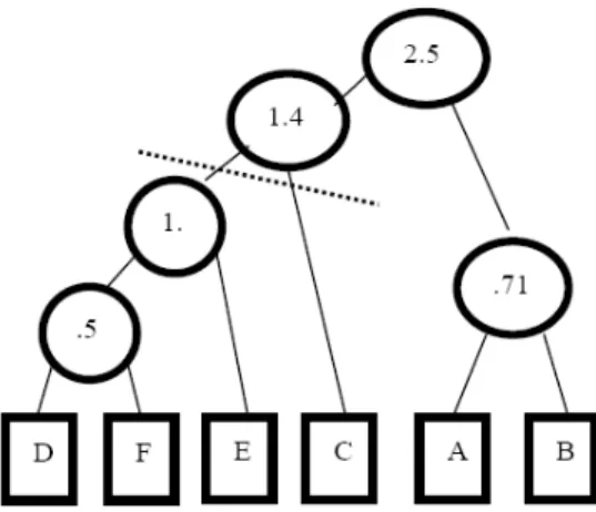
The iterations for generating Binary Tree using single linkage are as follows:
1. Cluster D and cluster F into (D,F) at distance 0.5 2. Merge cluster A and cluster B into (A, B) at 0.71 3. Merge cluster E and (D, F) into ((D, F), E) at 1.00 4. Merge cluster ((D, F), E) and C into (((D, F), E), C) at distance 1.41
5. Merge cluster (((D, F), E), C) and (A, B) into ((((D, F),E), C), (A, B)) at distance 2.50
The iterations for generating Binary Tree using complete linkage are as follows:
1. Cluster A and Cluster C into (A, C) at distance 5.6.AC distance is 5.6
2. BE distance is 3.5 3. ACF distance is 2.5 4. BED distance is 1.0 5. ACFBED distance is 0.5
The obtained distance matrix and cophenetic distance matrix are represented in Table 2 and Table 3. In this paper, distance matrix calculated only once (i.e in first iteration). Cophenetic distance matrix get values at the end of each iteration. For both matrices we need to fill only the
lower triangular values. Complete matrix representation is given here.
Table 2. Distance Matrix
0
0.71
5.66
3.61
4.24
3.2
0.71
0
4.95
2.92
3.54
2.5
5.66
4.95
0
2.24
1.41
2.5
3.61
2.92
2.24
0
1
0.5
4.24
3.54
1.41
1
0
1.12
3.2
2.5
2.5
0.5
1.12
0
Table 3. Cophenetic Distance Matrix
0
0.71
2.5
2.5
2.5
2.5
0.71
0
2.5
2.5
2.5
2.5
2.5
2.5
0
1.41
1.41
1.41
2.5
2.5
1.41
0
1
0.5
2.5
2.5
1.41
1
0
1
2.5
2.5
1.41
0.5
1
0
Cophenetic Correlation Coefficient is simply correlation coefficient between distance matrix and Cophenetic matrix, Correl (Dist, CPCC). In our example Correl (Dist, CPCC)= 86.39%. As the value of the Cophenetic Correlation Coefficient is close to 100%, that the clustering is good. Refer Figure 8.
Table 4. Linkage Measures Vs Cophenentic Correlation Coefficient
Techniques CPCC
Single Link 0.863
Complete Link 0.539
In our example we take yeast cell dataset with eight different attributes are clustered into ten groups.
5. CONCLUSIONS
be represented in single dimensional array, even when large databases are used. And, we represent the cluster results as a binary tree which gives clear grouping. Cut distance is used to find the number of clusters and clustered objects. The results are verified with Cophenetic correlation coefficient validation index. Hierarchical clustering method suffers from its inability to perform adjustment, once a m erge or split decision has been executed. This limitation can be overcome by the integration of hierarchal agglomeration with iterative relocation methods, as recent studies have emphasized. So, we plan to implement hierarchical clustering combining with other techniques and also to implement the parallel version of it, in future.
References
[1] Akinobu Sugiyama., Manabu Kotani., 2002, Analysis of gene expression Data Using Self-organizing Maps and k-means Clustering, IEEE, 1342-1345.
[2] Alon. U, Barkai, D.A., Notterman, K., Gish, S., Ybarra, D., Mack, and Levine, A.J., 1999, Broad Patterns of Gene Expression Revealed by Clustering Analysis of Tumor and Normal Colon Tissues Probed by Oligonucleotide Arrays, In Proc. Natl. Academy of Sciences, 96, 6745-6750.
[3] Ao. S.I, Kevin Y.P, Michael Ng, David Cheung, Fong .P, Ian Melhado and Sham. C., 2005, CLUSTAG: hierarchical clustering and graph methods for selecting SNPs, Oxford University press, 21(5), 1735-1736.[4] Bandyopadhyay, S., and Maulik, U., 2002. An evolutionary technique based on K -means algorithm for optimal clustering in RN, Information Science, 146, 221–237. [5] Cheng Y., Church GM., 2000, Biclustering of expression data. Proceedings of the Eighth International Conference on Intelligent Systems for Molecular Biology (ISMB), 8:93–103, 2000.
[6] Chen, C.Y., and Ye, F., 2004. Particle swarm optimization algorithm and its application to clustering analysis. In Proceedings of the 2004 I EEE International Conference on Networking, Sensing and Control, 789–794.
[7] Clark, F., Olson, 1995, Parallel algorithms for hierarchical clustering Parallel Computing, 21, 1313-1325
[8] Day, W.H,E., and Edelsbrunner, H., 1984, Efficient algorithms for agglomerative hierarchical clustering methods, J. Classification, l(1), 7-24. [9] Defays, D., 1977, An efficient algorithm for a complete link method, Comput. J, 20, 364-366 [10] Du. Z, Lin. F, 2005, A novel parallelization approach for hierarchical clustering. Parallel Computing, 31, 523-527. [11] Duran B. S. and Odell. B. S., 1974, Cluster Analysis, A Survey, volume 100 of Lectures Notes in Economics and Mathematical Systems. Springer.
[12] Eisen M., Spellman P., Brown P., Botstein D., 1998, Cluster analysis and display of genome-wide expression patterns. In Proc Natl. Acad. Science USA, 95(25), 14863-14868.
[13] Eisen, M.B., Brown, P.O., 1999, DNA arrays of gene expression, In: methods in enzymology, 303, 179-205.
[14] Getz G., Levine E., and Domany E.,, 2000, Coupled two-way clustering analysis of gene microarray data. In Proc. Natl. Acad. Sci. USA, 97(22), 12079–12084.
[15] Han, J.W., and Kamber. M., 2001, Data Mining Concepts and Techniques. Higher Education Press, Beijing.
[16] Hisashi Koga., Tetsuo Ishibashi., ToshinoriWatanabe., 2007, Fast agglomerative hierarchical clustering algorithm using Locality-Sensitive Hashing, Knowledge Inf. Syst. 12(1), 25–53.
Sadiq Hussain MCA from Tezpur University, Assam,India in the year 2000 w ith CGPA 7.85. Currently, he i s working as System Administrator of Dibrugarh University. He is in this position since December, 2008. He is in the charge of Computerization of Examination System and MIS of Dibrugarh University.
Pro Prof.G.C. Hazarika
Date of birth : 01-01-1954
Academic Qualification : M.Sc. (Math.), Ph.D. (Math). Positions held :
Director i/c, Centre for Computer Studies, Dibrugarh University, and
Professor, Department of Mathematics, Dibrugarh University Academic Positions held:
a.Computer Programmer: Joined as Computer Programmer, Dibrugarh University Computer Centre in Dec, 1977 and served till April, 1985.
b.Lecturer: Joined as Lecturer in the Department of Mathematics, Dibrugarh University in April, 1985.
c.Reader: Joined as Reader in a regular post in June, 1990. d.Professor: Joined as Professor in a regular post in August, 1998. Publications (a few)
1.Magnatic effect on flow through circular tube of non-uniform cross section with permeable walls
- Applied Science Periodical Vol. V. No.1, February, 2003 Jointly with B.C. Bhuyan.
2.Influence of Magnetic filed on Separation of a Binary Fluid Mixture in Free Convection flow Considering Soret Effect
- J. Nat. Acad. Math. Vol. 20 (2006), pp. 1-20 Jointly with B.R. Sharma and R.N. Singh
3. Effects of Variable viscosity and Thermal Conductivity on flow and heat transfer of a Stretching Surface of a rotating micropolar fluid with suction and blowing
- Bull. Pure and Appl. Sc. – Vol.-25 E No. 2, PP-361-370, 2006.
Jointly with P.J. Borthakur.
4. Effects of Variable viscosity and Thermal Conductivity on boundary Layer flow and heat transfer of micropolar fluid near an axisyusmetric Stagnation point on a moving cylinder- Proc. 51st . cong. of ISTAM, Dec-2006.
Research experiment:
Have guiles 11 Ph. D students and 9 M Phil students