Rev. Bras. Econ. vol.71 número1

(1)

Development Accounting, the Elasticity of

Substitution, and Non-neutral

Technological Change

Marcelo de Albuquerque e Mello

*,†

André de Souza Rodrigues

‡

Contents: 1. Introduction; 2. Related Literature; 3. Methodology; 4. Data; 5. Estimates ; 6. Robustness Check; 7. Conclusion; Appendix. Lists and Tables.

Keywords: Development Accounting, Elasticity of Substitution, Non-Neutral Technological Change, CES Technology.

JEL Code: O40, O47.

We apply the tools of development accounting to a broad panel over the period 1970–2014. However, we depart from the traditional Cobb–Douglas hypoth-esis with Hicks-neutral technological change, and assume a CES technology, which allows for a constant but non-unitary elasticity of substitution, and for non-neutral technological change. For different values of the elasticity of sub-stitution, and different representations of technological change, we ﬁnd that the cross-country variation in GDP per worker accounted for by factor inputs is decreasing over time until the mid-2000s, when it reverses its trend. In ad-dition, we ﬁnd that in the recent period technology accounts for up to 80% of the cross-country variation in GDP per worker.

Nós aplicamos as técnicas de contabilidade do desenvolvimento em um amplo pai-nel de países no período 1970–2014. Entretanto, nós desviamos da tradicional hipó-tese da Cobb–Douglas com progresso tecnológico Hicks-neutro, e assumimos uma tecnologia CES, que permite elasticidade de substituição constante, porém diferente da unidade, e progresso tecnológico não-neutro. Para diferentes valores da elastici-dade de substituição, e diferentes representações do progresso tecnológico, nossas estimativas sugerem que a variação no PIB por trabalhador entre países que pode ser explicada pela variação nos fatores de produção é decrescente ao longo do tempo até a metade dos anos 2000s, quando essa tendência é revertida. Adicionalmente, nossas estimativas sugerem que no período recente diferenças na tecnologia entre os países explicam cerca de 80% da variação do PIB per capita entre os países.

*_{Departamento de Economia, Ibmec/RJ and Universidade Estadual do Rio de Janeiro (UERJ). Av. Presidente Wilson 118/1,115, Rio}

de Janeiro, RJ, Brasil. CEP 20030-020. Tel+55 21 4503-4161. Fax+55 21 4503-4168. Email:mmello2@ibmec.edu.br

†_{I would like to thank Christiano Arrigoni, Rodrigo Novinski, Per Axelson, and seminar participants at Ibmec/RJ for helpful}

comments. Finally, all errors are ours.

(2)

1. INTRODUCTION

The current consensus in the Development Accounting literature establishes that the breakdown

tech-nology vs. inputs is “50-50”, (seeCaselli,2005, for instance). That is, 50% of the cross-country variance

in GDP per worker can be accounted for by cross-country differences in technology, and the remainder 50% can be accounted for by cross-country differences in factor inputs. However, this consensus rests largely on cross-section exercises with the Cobb–Douglas assumption.

In fact, the Cobb–Douglas (CD) production function is the number one choice to represent the aggregate technology in development accounting exercises. In general, one justiﬁes the CD assumption on grounds that its property of constant factor shares matches the data. However, the evidence in

Bernanke & Gurkaynak(2001) suggests that labor shares vary substantially across countries. If indeed factor shares vary across countries, then the CD assumption may not be the best representation for the aggregate technology.

In addition to its property of constant factor shares, the CD production function restricts the

elas-ticity of substitution between capital and labor, henceforth denoted byσ, to be constant and equal to

one. Whether or notσ is unitary is an empirical question. And, the empirical evidence does not support

an unitaryσ. For instance, for a panel of 82 countries over the period 1960–1987,Duffy & Papageorgiou

(2000) ﬁnd evidence thatσ is well above unity, whereasMello(2015), for a panel of 100 countries over

the period 1970–2008, ﬁnds estimates ofσ that are below unity. The value of the elasticity of

substitu-tion matters for development accounting exercises and, therefore, getting the appropriate value forσ

is important.

Another restriction of the CD production function is that differences in technology arise in a neu-tral, or bias-free, form. This restriction derives from the property of the CD, which is the only pro-duction function in which the three forms of technological change—Hicks neutral, Solow neutral, and Harrod neutral—are equivalent. This can be shown as follows. Take a CD with Harrod-neutral

(labor-augmenting) technological change:Y₌Kα(_AhL)1−α

. It is easy to see that this CD is equivalent to a CD

with Hicks-neutral technological change, such as thisY ₌A1−α_Kα(_hL)1−α

, which is also equivalent to

a CD with Solow neutral (capital-augmenting) technological change,Y ₌(_A1−_αα_K)α(_hL)1−α

. That is, in the three cases above, technology enters equivalently in a multiplicative form.

One of the implications of this restriction is that if one country is technologically more advanced than another is, then it must use all its factor inputs more efficiently than the other country does. There-fore, a situation in which one country uses capital more efficiently than the other does, while it uses human capital less efficiently, cannot be identified when one assumes a CD production function.

The problem with this is that the evidence suggests that the efﬁciency with which factor inputs

are used varies across countries. According to the evidence inCaselli & Coleman II(2006), rich countries

use skilled labor more efﬁciently than poor countries do, whereas poor countries use unskilled labor

more efﬁciently. Similarly,Caselli(2005) presents evidence that rich countries use human capital more

efﬁciently than poor countries do. In order to identify these differences we need to depart from the CD world.

If indeed the elasticity of substitution differs from unity and factor-efﬁciency is non-neutral, as the empirical evidence suggests, then performing development accounting exercises relaxing these two con-straints may change the consensus view, and, consequently, may change any policy implications derived from the exercise. These two restrictions—unitary elasticity of substitution and factor neutrality—can be relaxed by assuming a Constant Elasticity of Substitution (CES) production function as representative of the aggregate technology. The CES is the simplest production function that allows for a constant but non-unitary elasticity of substitution and non-neutral technological progress.

(3)

in the data by applying the tools of development accounting on the time series for GDP per worker from 1970 to 2014, instead of focusing on a speciﬁc year as in traditional cross-section studies in the literature.

We construct a panel with data on 84 countries over the period 1970–2014 from the latest version of the PWT, version 9.0. Our estimates suggest that the proportion of the cross-country variability in GDP per worker that can be accounted for by the cross-country variability in factor inputs exhibits a persistent decreasing trend. However, from 2005 towards the end of the sample period, it exhibits a soft increasing trend. In the more recent period, the technology-input breakdown is about “80-20” in favor of technology as the key factor behind the huge observed international variation in GDP per worker. This is a big departure from the “50-50” consensus. Moreover, this ﬁnding is robust to different values of the elasticity of substitution, and different representations of technological progress.

Additionally, as a robustness check, we construct two panels with data from PWT 8.1 and PWT 7.0 and apply the same development accounting tools to these panels. Our initial ﬁndings are corroborated when we use data from PWT 8.1, and corroborated to a lesser extent when we use data from PWT 7.0. Interestingly, the explanatory power of factors of production as a key determinant of the cross-country variance in GDP per worker is greater when we use data from PWT 9.0 and PWT 8.1.

We contribute to the debate by shedding light on the proximate causes of economic growth. In

particular, our study relates toCaselli(2005),Aiyar & Dalgaard (2009),Mello (2009), Ferreira, Pessoa,

& Veloso(2008), andArezki & Cherif(2010). We use the traditional tools of development accounting

exercises applied to cross-sectional data, as inCaselli(2005), and apply them on a panel data setting,

exploring the time variation in the data as inMello(2009),Ferreira et al.(2008), andArezki & Cherif

(2010). Moreover, we study the sensitivity of development accounting exercises with respect to the

value of the elasticity of substitution in the representative aggregate technology as inAiyar & Dalgaard

(2009), and the effects of non-neutral technological change as inCaselli & Coleman II(2006), andArezki

& Cherif(2010). Additionally, we explore the latest version of Penn World Tables dataset (version 9.0), as well as earlier versions of this dataset (versions 8.1 and 7.0).

We structure this article as follows. Insection 2, we brieﬂy review the literature. Insection 3, we

present our methodology, describing how we can decompose a CES production function into a

factor-only component, and a technology component. Insection 4, we present our data. Insection 5, we

present our estimates of the successes measures of the factor-only model for the PWT version 9.0. On

section 6, we present estimates of the measures of success of the factor-only model for data from PWT

versions 8.1 and 7.0, as a robustness check. Finally,section 7concludes.

2. RELATED LITERATURE

The debate about the determinants of the huge observed cross-country income differences, whether it

is the technology or factor inputs, goes back to the late 1960s (Caselli,2008). However, it was not until

the publication ofKlenow & Rodríguez-Clare(1997) that the tools and tricks of development accounting

were popularized.

Development accounting is to cross-section data, what growth accounting is to time series data. In a growth accounting exercise one computes, over a period of time, the growth rate of output and factor inputs, and estimate the growth in total factor productivity (TFP) as a residual. The exercise is helpful to identify the sources of growth, whether it comes from inputs or TFP. If growth in output comes from inputs, then it is likely to be temporary, whereas if it comes from TFP then it can be long lasting.

(4)

The decomposition exercise can give insight into the proximate causes of growth. By identify-ing the sources of cross-country variability in GDP per worker one can think about policies aimed at reducing inequality among nations. For instance, if one ﬁnds that the quantity of factor inputs can ac-count for a large portion of the cross-ac-country variability in output per worker, then, instead of focusing on technology, policy makers should look into the causes of low accumulation of factor inputs across countries.

Caselli(2005), the most cited survey in the literature, performs a series of development account-ing exercises for a cross-section of 94 countries in the year 1996 with data from Penn World Tables version 6.1. His estimates suggest the breakdown factor inputs versus technology is about “50-50”.

According toHsieh & Klenow(2010), another recent survey, the current consensus establishes that

tech-nology accounts for 50-70% of the cross-country differences in GDP per worker.

In our decomposition exercise, we break down GDP per worker in terms of the capital-output

ratio, as inKlenow & Rodríguez-Clare(1997), among others. Moreover, to assess the role of factor

in-puts vis-à-vis technology in accounting for cross-country output differences, we use the methodology inCaselli(2005). Furthermore, we followMello(2009),Ferreira et al.(2008), andArezki & Cherif(2010) in constructing a panel and exploring the time variation in the data, instead of looking at a single point in time as in much of the literature.

3. METHODOLOGY

We represent the aggregate technology by a CES production function as follows:

Y₌(_αKσσ−1₊(₁−_α)(AhL₎σσ−1)

σ σ−1

, (1)

whereY is output,Kis physical capital,Ais Harrod-neutral (labor-augmenting) technological progress,

h is human capital per worker, and Lis the number of workers. The elasticity of substitution given

by the parameter σ. Ifσ =1 we are back to the Cobb–Douglas world, in which output is given by

Y₌Kα(AhL)1−α

. Aiyar & Dalgaard(2009) also adopt the above functional form.

Based on the production function in (1), we can break down output per worker into two

compo-nents, a factor-only component, and a technology component:

Y

L =

* ,

1−_α

1−_α(K/Y)σσ−1

+

-σ σ−1

Ah. (2)

In this case, the factor-only model is given by

yKH=* ,

1−_α

1−_α(_K_/_Y)σσ−1

+

-σ σ−1

. (3)

In the CD case, i.e., ifσ=1, the factor-only model is given by

yKH=

(_K

Y

)1α−α

h_. (4)

Equation (4) is the well-knownKlenow & Rodríguez-Clare(1997) break-down.

The speciﬁcation in (1) assumes that technological change is Harrod-neutral or labor

augment-ing. However, we can extend this speciﬁcation to include non-neutral technological change. Following

Aiyar & Dalgaard(2009), we assume a CES that allows for Harrod (labor) and Solow (capital) neutral technological change:

Y₌(_α₍BK₎σσ−1

+(1−_α)(AhL₎σσ−1)

σ σ−1

(5)

where B denotes the Solow neutral (capital augmenting) technological change, and A denotes the

Harrod-neutral (labor augmenting) technological change. We can rearrange equation (5) and break it

down into two components, just like we did with equation (1). We obtain the following expression:

Y

L =

* ,

1−_α

1−_α[B₍K/Y₎]σσ−1

+

-σ σ−1

Ah. (6)

The problem with the above decomposition is that the capital augmenting parameterB is included in

the factor-only component. That is, in practice, we have not separated the technology component from

the factor-only component. In order to obtain a feasible decomposition based on equation (6), we need

to ﬁnd a way to estimate or “ﬁx” the capital augmenting parameterB.

We follow the strategy inCaselli & Coleman II(2006), which is also adopted byAiyar & Dalgaard

(2009). The idea is, ﬁrst, to ﬁx the parameterB at the “technological frontier”, which is taken to be the

U.S. level. Second, given competitive markets and the production function in equation (5), we can write

the capital share as follows:

Sk=αB

σ−1

σ (_K_/_Y) σ−1

σ _, (7)

whereSkdenotes the capital share. The trick here is to assume that all countries have access to the

tech-nological frontier. That is, all countries have access to the same (U.S.) parameterB. From equation (7),

we can estimate the parameterB as follows:

αBσσ−1 ₌SUS

K

(_YUS

KUS

)σσ−1

, (8)

where the variables with the superscript denote their U.S. levels. Implementing this strategy, when

technological change is both Harrod and Solow neutral, the factor-only model, denoted byyABKH, is given

by:

yABKH=*..

,

1−_α

1−SUS

K

(YUS KUS

)σσ−1(K Y

)σσ−1

+/ /

-σ σ−1

h. (9)

With the exception of the non-observable parameterB, which we estimate with equation (8), all

other variables in equation (9) can be directly obtained from PWT dataset, or can be constructed from

the variables therein.

The ﬁrst measure of success of the factor-only model we look at is the ratio of the variance of the log of the factor-only model to the variance of the log of GDP per worker. We denote this measure of

success byS1:

S1₌Var

(_Log( yKH) ) Var(

Log(y)) . (10)

As correctly pointed out inCaselli(2005), theS1 measure is sensitive to extreme values, which

may contaminate the analysis. In this sense,Caselli(2005) also considers a second measure of success,

denoted byS2, which takes the ratio of the 90thto 10thpercentile ratio of the factor-only model to the

90th_{to 10}th_{percentile of the observed GDP per worker. The}_S2_{measure is given by}

S2=y 90th KH /yKH10th

Y90th_/_Y10th, (11)

whereyKH90th andy10thKH denote, respectively, the level of GDP per worker of the factor-only model at the

90th_{and the 10}th_{percentile, and}_Y90th_and_Y10th_{denote the observed level of GDP per worker at the 90}th

(6)

4. DATA

We construct our main panel with data from the latest version of Penn World Tables (PWT) dataset version 9.0. Our panel includes 84 countries for which population is equal to or greater than 1 million in 1985, and the time series for the variables we use are complete over the period 1970–2014.

Our measure of output is the variableRGDPO(output-side real GDP at chained PPP in millions of

2005 USD), the measure for the aggregate stock of capital is the variableCK (capital stock at PPP in

millions of 2005 USD), and the measure of workers is the variableEMP(number of individuals engaged

in production). GDP per worker is calculated as the ratio ofRGDPO/EMP, and the capital-output ratio is

computed asCK/RGDPO.

Our measure of human capital is the variablehcin PWT 9.0, which is an index of human capital

per person, based on years of schooling, fromBarro & Lee(2010) dataset, and returns to education, from

Psacharopoulos(1994). This measure of human capital is also used in the PWT 8.1.

In addition to the PWT version 9.0, as a robustness check, we work with two other versions of PWT, versions 8.1 and 7.0. For the PWT 8.1, our panel includes 77 countries for which population is greater than or equal to 1 million in 1985, and the time series for the variables is complete over the period 1970–2011.

For the PWT 7.0, we construct a panel with 85 countries for the period 1970–2008. For this panel,

we compute the number of workers asRGDPCH*POP/RGDPWOK, where we denote the variables by their

PWT 7.0 codes. Real GDP (Y_{) is constructed by multiplying the series} RGDPWOK2 _{by the number of}

workers. The seriesRGDPWOK2is given byRGDPL2WOK=RGDPL2*POP/Workers, whereRGDPL2is an

updated version ofRGDPLwhich is real GDP (Laspeyre index).

In order to construct the time series for the physical capital stock, we followMello(2009) and

use the perpetual inventory method. The initial value of aggregate capital is set atI₀/(д+δ), where

I₀ is initial investment (measured as the investment in the ﬁrst year for which data is available),_д is

the average growth rate in investment for the ﬁrst year for which data is available until 1970, andδis

the depreciation rate which we set at 6%. GivenK₀,Kt evolves according to the capital accumulation

equation, namely,Kt₌(1−δ)Kt−1+It. To ensure the quality of capital stock estimates, we initiate the

series on the ﬁrst year for which data is available and discard all observations until 1969. By discarding

the initial years, we guard ourselves against a bad initial guess. SeeMello(2009) for more details.

Our measure of human capital for the PWT 7.0, uses the average years of schooling for the

popula-tion 25 years old or older obtained fromBarro & Lee(2010) dataset. Speciﬁcally, we assume that human

capitalH _{is given by}H ₌e0.1∗uL

, whereu _{is the average years of schooling and}L _{is the number of}

workers. That is, we assume that the Mincerian coefﬁcient of returns to education is 0.1 for all countries.

In theAppendix, we provide the complete list of countries in the three panels that we use, PWT 9.0,

PWT 8.1, and PWT 7.0, as well as the list of countries considered rich/poor, as deﬁned in the next section. Our dataset is available upon request.

5. ESTIMATES

We initially analyze estimates of theS1measure for the case in which technological change is Harrod

neutral only. We assume different values for the elasticity of substitution according to the empirical

evidence. The exercises are performed forσ=1.5, according to the evidence inDuffy & Papageorgiou

(2000), forσ=0.8 according to the evidence inMello(2015), andAiyar & Dalgaard(2009), forσ=0.5

according toAntràs(2004), and as a benchmark forσ=1, which is the Cobb–Douglas case.1

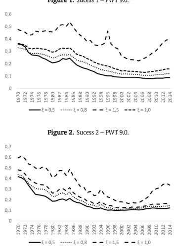
Figure 1displays the S1 measure for a CES with Harrod neutral technological change for data from PWT 9.0. It contains at least four salient features. First, we observe that the higher the elasticity

(7)

of substitution the higher the explanatory power of the factor-only model. In particular, the explanatory

power of the factor-only model withσ=1.5 is about twenty percentage points higher than withσ=

0.5. Second, for values of the elasticity of substitution equal to or less than one, the factor-only model

explains a much lower percentage than the 50% consensus. For instance, forσ=0.80, the factor-only

model explains about 30% of the cross-country variation in GDP per worker in the mid-1970s, and it

decreases to about 10% in the mid-1990s. Only if we assume thatσ=1.5, that theS1measure comes

close to the 50% consensus, but it still trails below the 50% for most of the sample period.

Third, the explanatory power of the factor-only model decreases over time. For instance, in 1970,

for σ≤₁, the factor-only model explains about 35% of the cross-country variation in GDP per worker.

Moreover, in 2000, forσ≤1, its explanatory power drops to less than 20%. Forσ=1.5, the explanatory

power of the factor-only model drops by about 20 percentage points over the period 1970–2005. This

ﬁnding is consistent with the estimates inFerreira et al.(2008), andArezki & Cherif(2010), who also ﬁnd

that the explanatory power of the factor-only is decreasing over time. Fourth, in the last eight years of the sample period, 2006–2014, the explanatory power of the factor-only model increases somewhat.

For example, in the case ofσ=1.5, it increases by more than 10 percentage points, while forσ=1it

increases by a few percentage points.

The observations above are conﬁrmed by examining theS2measure of success. As can be seen in

Figure 2, the pattern ofS2mimics that ofS1, so that the four observations we made aboutS1inFigure 1

also apply toS2inFigure 2. One noticeable difference is that, for the entire sample period, according to

Figure 1.Sucess 1 – PWT 9.0.

0 0,1 0,2 0,3 0,4 0,5 0,6 1 9 7 0 1 9 7 2 1 9 7 4 1 9 7 6 1 9 7 8 1 9 8 0 1 9 8 2 1 9 8 4 1 9 8 6 1 9 8 8 1 9 9 0 1 9 9 2 1 9 9 4 1 9 9 6 1 9 9 8 2 0 0 0 2 0 0 2 2 0 0 4 2 0 0 6 2 0 0 8 2 0 1 0 2 0 1 2 2 0 1 4

‡AìUñ ‡AìUô ‡AíUñ ‡AíUì

0 0,1 0,2 0,3 0,4 0,5 0,6 0,7 1 9 7 0 1 9 7 2 1 9 7 4 1 9 7 6 1 9 7 8 1 9 8 0 1 9 8 2 1 9 8 4 1 9 8 6 1 9 8 8 1 9 9 0 1 9 9 2 1 9 9 4 1 9 9 6 1 9 9 8 2 0 0 0 2 0 0 2 2 0 0 4 2 0 0 6 2 0 0 8 2 0 1 0 2 0 1 2 2 0 1 4

(8)

theS2measure, the explanatory power of the factor-only model is, on average, ﬁve percentage points

greater than compared to theS1measure.

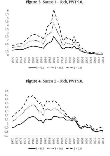
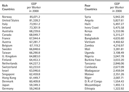
In order to learn more about the cross-country variability in GDP per worker, we segment the sample in three parts: rich, middle-income, and poor countries. We consider rich the 21 countries (top 25%) in our panel with the highest level of GDP per worker in the year 2000. The list of rich countries

can be found inTable A-1in theAppendix. Figure 3displays theS1for measure for the sub-sample of

rich countries.

We only report the S1 measure for rich countries forσ≤1, because S1 estimates for σ =1.5

generate too much variability, well above the observed variability in the data. For instance, in the year

1991, the variability generated by theS1measure forσ=1.5is a factor of 12 of the observed variability

in observed GDP per worker. In order to avoid any distortion in the ﬁgure with such large realizations

we omit theS1estimates forσ=1.5. These estimates are available upon request.

TheS1measure forσ=0.8andσ=1, as shown inFigure 3, generates more variability than what

is observed in the data for most of the sample period. In particular, forσ=0.8 the factor-only model

fully accounts for the variability in the data until 2002, and forσ=1, until 2003. Forσ =0.5, theS1

measure practically explains all of the variability in the data from 1978 to 2000. Interestingly, starting

in the early 2000s, the S1measure for rich countries for any value ofσ loses explanatory power fast,

reaching 2014 in the range 10%–24%.

The ﬁnding that the factor-only model has a higher explanatory power for rich countries is in-tuitive. After all, for rich countries the observed cross-sectional variance of GDP per worker must be smaller than for the panel as a whole. Additionally, it is plausible to assume that rich countries have access to same technology, and, if so, then cross-sectional differences in GDP per worker must come from cross-sectional differences in factor inputs.

If indeed the source of the cross-sectional differences in GDP per worker are cross-sectional differ-ences in factor inputs, then it is easier for the policy maker to design policies to reduce income inequality. The reason being is that differences in technology can come from many sources, such as credit market imperfections or judicial uncertainty, while differences in factor inputs can be reduced via accumulation of capital, with a high investment rate.

Figure 4displays the S2 measure for rich countries, including S2 estimates for σ =1.5. The

explanatory power of the factor-only model is greater forσ=1.5. The range ofS2estimates forσ=1.5

goes from 1.04 to 2.75, while the range ofS1 for rich countries, forσ =1.5, goes from 1.47 to 13.2,

which suggests that theS1measure is in fact contaminated with extreme values and a higher elasticity

of substitution magniﬁes the effects of outliers. Other than that, the general pattern exhibited by the

S2measure inFigure 4forσ≤₁mimics the pattern we observe for the_S1measure inFigure 3.

As in the case for the panel as a whole, the explanatory power ofS2decreases over time. However,

until 2001 it generates enough variability to match the data. Interestingly, the loss in explanatory power

is small and it only occurs forσ≤₁. In general, we can say that the factor-only model accounts well for

the cross-sectional variability in GDP per worker for rich countries.

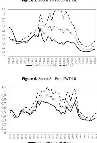
Figures5and6display theS1 and S2measures for poor countries, respectively. We classify as

poor countries the bottom 21 countries (25% of the panel) ranked according to their GDP per worker in

year 2000. The list of countries classiﬁed as poor is in theAppendix.

Figure 5displays theS1measure for poor countries. Again, we omit from theS1estimates for

σ =1.5 due to extreme values. The estimates inFigure 5show a hump-shaped form, with the hump

formed between 1985 and 2000. For the years 1970–1984, theS1estimates fall in the range 35%–60%,

and increase over time. In the second period, 1985–2000, forσ=1,S1increases and even goes above 1;

forσ=0.8,S1estimates hover around 60%; and forσ=0.5,S1estimates decreases below 40%. For

the end of the sample period, 2001–2014,S1estimates decrease fast, reaching low 10s% and 20s%, just

(9)

Figure 3.Sucess 1 – Rich, PWT 9.0. 0 0,5 1 1,5 2 2,5 3 3,5 4 4,5 5 5,5 6 1 9 7 0 1 9 7 2 1 9 7 4 1 9 7 6 1 9 7 8 1 9 8 0 1 9 8 2 1 9 8 4 1 9 8 6 1 9 8 8 1 9 9 0 1 9 9 2 1 9 9 4 1 9 9 6 1 9 9 8 2 0 0 0 2 0 0 2 2 0 0 4 2 0 0 6 2 0 0 8 2 0 1 0 2 0 1 2 2 0 1 4

‡AìUñ ‡AìUô ‡AíUì

Figure 4.Sucess 2 – Rich, PWT 9.0.

0,7 0,8 0,9 1 1,1 1,2 1,3 1,4 1,5 1,6 1,7 1,8 1 9 7 0 1 9 7 2 1 9 7 4 1 9 7 6 1 9 7 8 1 9 8 0 1 9 8 2 1 9 8 4 1 9 8 6 1 9 8 8 1 9 9 0 1 9 9 2 1 9 9 4 1 9 9 6 1 9 9 8 2 0 0 0 2 0 0 2 2 0 0 4 2 0 0 6 2 0 0 8 2 0 1 0 2 0 1 2 2 0 1 4

Figure 6displays the estimates ofS2for poor countries, excluding estimates forσ =1.5. Again,

S2estimates forσ=1.5exhibit a lot of variability, being above one for most of the sample period, 1981–

2005. For other values of the elasticity of substitution, the pattern we observe inFigure 6is consistent

with the one inFigure 5. That is, forσ≤₁, we observe a hump-shaped form, with the hump between

the years 1985–2000. Additionally, the range of estimates is similar to the range of estimates inFigure 5,

with the explanatory power of the factor-only model oscillating around 50% in the beginning of the

sample period, reaching 100% forσ=1around 1990, and settling at 35%–45% at the end of the sample

period.

Based on ﬁgures5and6, we conclude that the factor-only model, forσ≤₁, accounts for 35%–45%

for the cross-country variation in GDP per worker, and for σ=1.5, it accounts for 50%–70%. That is,

the elasticity of substitution does affect the explanatory power of the factor-only model. However, it does not lead it too far off from the “50-50” consensus.

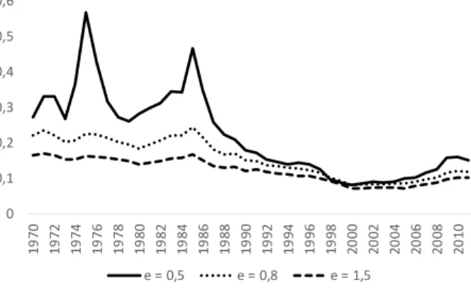
Figure 7displaysS1estimates for the case in which technological progress is non-neutral, that is,

it is Harrod and Solow neutral. Estimates ofS1forσ=0.5andσ=0.8, inFigure 7, exhibit a decreasing

trend, starting in the low 40s% and falling in the range of 10s% and 20s% towards the end of the sample

period. Estimates ofS1, forσ=1.5, also exhibit a decreasing trend. However, it starts in the low 20s%

and reach the 10% around year 2000, when it starts to increase towards 15%. Additionally, for most

(10)

Figure 5.Sucess 1 – Poor, PWT 9.0. 0 0,1 0,2 0,3 0,4 0,5 0,6 0,7 0,8 0,9 1 1,1 1 9 7 0 1 9 7 2 1 9 7 4 1 9 7 6 1 9 7 8 1 9 8 0 1 9 8 2 1 9 8 4 1 9 8 6 1 9 8 8 1 9 9 0 1 9 9 2 1 9 9 4 1 9 9 6 1 9 9 8 2 0 0 0 2 0 0 2 2 0 0 4 2 0 0 6 2 0 0 8 2 0 1 0 2 0 1 2 2 0 1 4

Figure 6.Sucess 2 – Poor, PWT 9.0.

0 0,1 0,2 0,3 0,4 0,5 0,6 0,7 0,8 0,9 1 1,1 1 9 7 0 1 9 7 2 1 9 7 4 1 9 7 6 1 9 7 8 1 9 8 0 1 9 8 2 1 9 8 4 1 9 8 6 1 9 8 8 1 9 9 0 1 9 9 2 1 9 9 4 1 9 9 6 1 9 9 8 2 0 0 0 2 0 0 2 2 0 0 4 2 0 0 6 2 0 0 8 2 0 1 0 2 0 1 2 2 0 1 4

in sharp contrast with the Harrod neutral only case, in which the explanatory power of the factor-only

model is greater withσ=1.5. Moreover, theS1estimates intersect at several points, suggesting that

S1is not monotonic with respect to the elasticity of substitution.

TheS2 measure for the Harrod and Solow neutral case, shown inFigure 8, mimics the pattern

seen inFigure 7. As before, the explanatory power of the factor-only model is decreasing over time, and

it is greatest whenσ=0.8. More speciﬁcally, the explanatory power of the factor-only model starts in

the range 30%–50%, and decreases over time to the range 10%–20%. The fall in the explanatory power of the factor-only model starts in the mid-1980s and it continues until the year 2000, just to increase slightly until 2014 and ﬁnish it around 15%.

Recall that to compute theS1 measure for the case of Harrod and Solow neutral technological

change, we assume that all countries have access to the U.S. capital augmenting technology. Note, however, that countries still differ in their labor augmenting technological change. Therefore, all the cross-country variability in technology comes from the cross-sectional variability in labor-augmenting technology. Thus, the decreasing explanatory power of the factor-only model is exactly matched by a larger role of cross-country differences in labor augmenting technology in accounting for cross-country income differences.

(11)

Figure 7.Sucess 1 – non-neutral Tech. Progress, PWT 9.0. 0 0,1 0,2 0,3 0,4 0,5 0,6 1 9 7 0 1 9 7 2 1 9 7 4 1 9 7 6 1 9 7 8 1 9 8 0 1 9 8 2 1 9 8 4 1 9 8 6 1 9 8 8 1 9 9 0 1 9 9 2 1 9 9 4 1 9 9 6 1 9 9 8 2 0 0 0 2 0 0 2 2 0 0 4 2 0 0 6 2 0 0 8 2 0 1 0 2 0 1 2 2 0 1 4

e = 0,5 e = 0,8 e = 1,5

Figure 8.Sucess 2 – non-neutral Tech. Progress, PWT 9.0.

0 0,1 0,2 0,3 0,4 0,5 0,6 1 9 7 0 1 9 7 2 1 9 7 4 1 9 7 6 1 9 7 8 1 9 8 0 1 9 8 2 1 9 8 4 1 9 8 6 1 9 8 8 1 9 9 0 1 9 9 2 1 9 9 4 1 9 9 6 1 9 9 8 2 0 0 0 2 0 0 2 2 0 0 4 2 0 0 6 2 0 0 8 2 0 1 0 2 0 1 2 2 0 1 4

e = 0,5 e = 0,8 e = 1,5

cross-country differences in GDP per worker are due to cross-country differences in the efﬁciency with which inputs are used. In particular, our estimates suggest that the current breakdown is “80-20” in favor of technology. These ﬁndings seem to be robust with respect to the different values of the elasticity of substitution and the form of technological change.

Any policy prescription aimed at reducing cross-country income differences should focus on the ability to convert inputs into output, that is, on efﬁciency, rather than on fostering the accumulation of inputs.

6. ROBUSTNESS CHECK

In this section, we check for robustness of our estimates by computing theS1 and S2 measures for

previous versions of the PWT dataset, namely, versions 8.1 and 7.0. We omit some of the ﬁgures here to economize on space (they are available upon request). We construct the panels using the same criteria

as insection 4, that is, by selecting countries for which the population in 1985 is above 1 million, and

data was available for the entire sample period, 1970–2011 for PWT 8.1, and 1970–2008 for PWT 7.0.

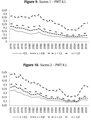
Figure 9displays theS1 measure for the PWT 8.1. First, the higher the elasticity of substitution the higher the explanatory power of the factor-only model. In particular, the explanatory power of the

factor-only model with σ=1.5 is about 20 percentage points higher than withσ =0.5. Second, for

values of the elasticity of substitution equal or less than one, the factor-only model explains a much

(12)

Figure 9.Sucess 1 – PWT 8.1. 0 0,05 0,1 0,15 0,2 0,25 0,3 0,35 0,4 0,45 1 9 7 0 1 9 7 2 1 9 7 4 1 9 7 6 1 9 7 8 1 9 8 0 1 9 8 2 1 9 8 4 1 9 8 6 1 9 8 8 1 9 9 0 1 9 9 2 1 9 9 4 1 9 9 6 1 9 9 8 2 0 0 0 2 0 0 2 2 0 0 4 2 0 0 6 2 0 0 8 2 0 1 0

1_AìUñ 1_AìUô 1_AíUñ 1_AíUì

0,05 0,1 0,15 0,2 0,25 0,3 0,35 0,4 0,45 1 9 7 0 1 9 7 2 1 9 7 4 1 9 7 6 1 9 7 8 1 9 8 0 1 9 8 2 1 9 8 4 1 9 8 6 1 9 8 8 1 9 9 0 1 9 9 2 1 9 9 4 1 9 9 6 1 9 9 8 2 0 0 0 2 0 0 2 2 0 0 4 2 0 0 6 2 0 0 8 2 0 1 0

1_AìUñ 1_AìUô 1_AíUñ 1_AíUì

about 30% of the cross-country variation in income per worker in the mid-1970s and it decreases to

about 10% in the mid-1990s. Only if we assume thatσ =1.5, that theS1 measure comes closer to

the 50% consensus, but it still trails below the 50% for most of the sample period. Lastly, estimates in

Figure 9are consistent with the ones we obtain with data from PWT 9.0.

We conﬁrm the above observations by examining theS2measure of success for PWT 8.1, as shown

inFigure 10. The pattern ofS2over time mimics that ofS1. Therefore, the same observations we made forFigure 9are also valid forFigure 10. One noticeable difference is that according to theS2measure, the explanatory power of the factor-only model averages about ﬁve percentage points higher than compared

with theS1measure.

Figures11and 12display, respectively, S1 and S2 estimates assuming a CES with non-neutral

technological change, and using data from PWT 8.1. The overall pattern ofS1inFigure 11is consistent

with the one inFigure 7. However, the explanatory power of the factor-only model is substantially

reduced when compared toFigure 7, which was constructed using data from PWT 9.0.

Probably the most interesting aspects in ﬁgures11and12are the decreasing trend inS1and the

end of period kick back. These two aspects that are also present in estimates from PWT 9.0.

As mentioned above, we do not present all the corresponding ﬁgures forS1andS2constructed

with data from PWT 7.0. Below, we present some of the estimates from PWT 7.0, comparing them with estimates from the more recent versions of the PWT.

Assuming Harrod neutral technological change only,Figure 13displaysS2estimates forσ=0.8

for three versions of the PWT we work with. As can be seen inFigure 13, in all cases the explanatory

(13)

in-Figure 11.Sucess 1 – non-neutral Tech. Progress, PWT 8.1. 0 0,1 0,2 0,3 0,4 0,5 0,6 1 9 7 0 1 9 7 2 1 9 7 4 1 9 7 6 1 9 7 8 1 9 8 0 1 9 8 2 1 9 8 4 1 9 8 6 1 9 8 8 1 9 9 0 1 9 9 2 1 9 9 4 1 9 9 6 1 9 9 8 2 0 0 0 2 0 0 2 2 0 0 4 2 0 0 6 2 0 0 8 2 0 1 0

e = 0,5 e = 0,8 e = 1,5

Figure 12.Sucess 2 – non-neutral Tech. Progress, PWT 8.1.

0,05 0,1 0,15 0,2 0,25 0,3 0,35 0,4 1 9 7 0 1 9 7 2 1 9 7 4 1 9 7 6 1 9 7 8 1 9 8 0 1 9 8 2 1 9 8 4 1 9 8 6 1 9 8 8 1 9 9 0 1 9 9 2 1 9 9 4 1 9 9 6 1 9 9 8 2 0 0 0 2 0 0 2 2 0 0 4 2 0 0 6 2 0 0 8 2 0 1 0

e = 0,5 e = 0,8 e = 1,5

crease. Interestingly, the explanatory power of the factor-only model is quite low when we use data from PWT 7.0. The explanatory power of the factor-only model is greater with data from PWT 9.0,

al-though from the mid-1990s towards the end of the sample period theS2measure has more or less the

same value whether computed with data from PWT 9.0 or PWT 8.1. These observations are also true for

S2estimates forσ=1.5assuming Harrod neutral technological change as shown inFigure 14.

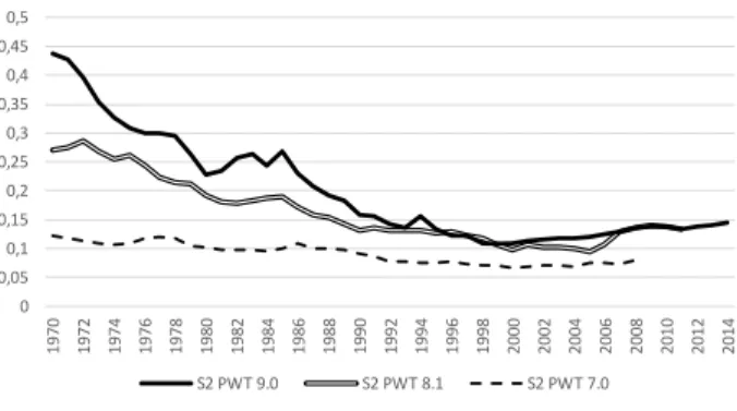
We also compute theS2measure, constructed assuming Harrod and Solow neutral technological

change, using data from the three versions of the PWT we work with. Figure 15displaysS2estimates

forσ=0.8. The decreasing trend inS2is present in all cases, less pronounced when we use data from

PWT 7.0, but very strong when we use data from PWT 9.0 and 8.1. Again, the explanatory power of the factor-only model is greater when we use data from PWT 9.0. Interestingly, around 1995 we observe

a convergence in S2 for data from PWT 9.0 and 8.1, with the explanatory power of the factor-only

oscillating between 10% and 15%. Furthermore, we observe the increase in the explanatory power of

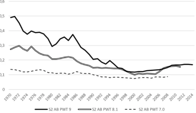
the factor-only from 2005. These observations are also valid forFigure 16, which displays estimates of

S2assuming Harrod and Solow neutral technological change andσ =1.5. We should only add that

forσ =1.5, the explanatory power of the factor-only model is some 20 percentage points lower than

(14)

Figure 13.ComparingS2Broad panelES=0.8.

0 0,05 0,1 0,15 0,2 0,25 0,3 0,35 0,4 0,45 0,5

1

9

7

0

1

9

7

2

1

9

7

4

1

9

7

6

1

9

7

8

1

9

8

0

1

9

8

2

1

9

8

4

1

9

8

6

1

9

8

1

9

0

1

9

2

1

9

4

1

9

6

1

9

8

2

0

2

0

2

0

4

2

0

6

2

0

8

2

0

1

0

2

0

1

2

0

1

4

S2 PWT 9.0 S2 PWT 8.1 S2 PWT 7.0

Figure 14.ComparingS2Broad panelES=1.5.

0 0,1 0,2 0,3 0,4 0,5 0,6 0,7

S2 PWT 9.0 S2 PWT 8.1 S2 PWT 7.0

7. CONCLUSION

We construct a broad panel with 84 countries over the period 1970–2014 with data from the latest version of PWT 9.0, and apply the tools of development accounting. We depart from two traditional assumptions commonly employed in the literature, namely, the Cobb–Douglas assumption and neutral technological change.

We adopt a CES production function that allows for a constant but non-unitary elasticity of sub-stitution and non-neutral technological change. Our estimates suggest that the explanatory power of the factor-only model exhibits a decreasing trend, with a soft kick back from 2005 to 2014. Additionally, when technological change is Harrod neutral the explanatory power of the factor-only model is greater

forσ=1.5, whereas when technological change is non-neutral the factor-only model explains more for

σ=0.8for PWT 9.0 data, and forσ=0.5 for PWT 8.1 data.

(15)

Figure 15.ComparingS2 ES=0.8Non-neutral T.Ch. – PWT 9.0, 8.1, 7.0.

0 0,1 0,2 0,3 0,4 0,5 0,6

S2 AB PWT 9 S2 AB PWT 8.1 S2 AB PWT 7.0

Figure 16.ComparingS2 ES=1.5Non-neutral T.Ch. – PWT 9.0, 8.1, 7.0.

0 0,05 0,1 0,15 0,2 0,25 0,3 0,35

S2 AB PWT 9 S2 AB PWT 8.1 S2 AB PWT 7.0

REFERENCES

Aiyar, S., & Dalgaard, C.-J. (2009). Accounting for productivity: Is it OK to assume that the world is Cobb–Douglas?

Journal of Macroeconomics,31, 290–303. doi:10.1016/j.jmacro.2008.09.007

Antràs, P. (2004). Is the U.S. aggregate production function Cobb–Douglas? New estimates of the elasticity of substitution.The B.E. Journal of Macroeconomics,4(1). doi:10.2202/1534-6005.1161

Arezki, R., & Cherif, R. (2010, April). Development accounting and the rise of TFP (IMF Working Paper No. WP/10/101). Washington, DC: International Monetary Fund. Retrieved fromhttps://www.imf.org/en/ Publications/WP/Issues/2016/12/31/Development-Accounting-and-the-Rise-of-TFP-23798

Barro, R. J., & Lee, J.-W. (2010, April).A new data set of educational attainment in the world, 1950–2010(Working Paper No. 15902). National Bureau of Economic Research (NBER). doi:10.3386/w15902

Bernanke, B. S., & Gurkaynak, R. S. (2001). Is growth exogenous? Taking Mankiw, Romer, and Weil seriously. In B. S. Bernanke & K. Rogoff (Eds.),NBER Macroeconomics Annual(pp. 11–57). Cambridge, MA: MIT Press. Caselli, F. (2005). Accounting for cross-country income differences. In P. Aghion & S. N. Durlauf (Eds.),Handbook

of economic growth(Vol. 1A, pp. 679–741). Elsevier. doi:10.1016/S1574-0684(05)01009-9

Caselli, F. (2008). Level accounting. In S. N. Durlauf & L. E. Blume (Eds.),The new Palgrave dictionary of economics. Palgrave Macmillan.

Caselli, F., & Coleman II, W. J. (2006). The world technology frontier. American Economic Review,96(3), 499–522.

(16)

Duffy, J., & Papageorgiou, C. (2000). A cross-country empirical investigation of the aggregate production function speciﬁcation.Journal of Economic Growth,5(1), 87–120. doi:10.1023/A:1009830421147

Ferreira, P. C., Pessoa, S. A., & Veloso, F. A. (2008). The evolution of international output differences (1970–2000): From factors to productivity.The B.E. Journal of Macroeconomics,8(1). doi:10.2202/1935-1690.1578 Hsieh, C.-T., & Klenow, P. J. (2010). Development accounting.American Economic Journal: Macroeconomics,2(1),

207–223. doi:10.1257/mac.2.1.207

Klenow, P. J., & Rodríguez-Clare, A. (1997). The neoclassical revival in growth economics: Has it gone too far? In B. S. Bernanke & J. J. Rotemberg (Eds.),NBER Macroeconomics Annual 1997, volume 12(pp. 73–114). MIT Press. Retrieved fromhttp://papers.nber.org/books/bern97-1

Mello, M. (2009). Estimates of the marginal product of capital, 1970-2000. The B.E. Journal of Macroeconomics, 9(1). doi:10.2202/1935-1690.1723

Mello, M. (2015).Another look at panel estimates of the elasticity of substitution.

Psacharopoulos, G. (1994). Returns to investment in education: A global update. World Development,22(9), 1325–1343. doi:10.1016/0305-750X(94)90007-8

APPENDIX. LISTS AND TABLES

Country List (All countries,

n

₌

₈₄

, PWT

9.0 )

Albania, Algeria, Angola, Argentina, Australia, Austria, Bangladesh, Belgium, Bolivia, Brazil, Bulgaria, Burkina Faso, Cambodia, Cameroon, Canada, Chile, China, Hong Kong, Colombia, Ivory Coast, Demo-cratic Republic of Congo, Denmark, Domenica Republic, Ecuador, Ethiopia, Finland, France, Germany, Ghana, Greece, Guatemala, Haiti, Honduras, Hungary, India, Indonesia, Iran, Iraq, Ireland, Israel, Italy, Japan, Kenya, Madagascar, Malawi, Malaysia, Mali, Mexico, Morocco, Mozambique, Netherlands, New Zealand, Niger, Nigeria, Norway, Pakistan, Paraguay, Peru, Philippines, Poland, Portugal, South Korea, Romania, Saudi Arabia, Senegal, Singapore, South Africa, Spain, Sri Lanka, Sweden, Switzerland, Syria, Taiwan, Thailand, Tunisia, Turkey, Tanzania, Uganda, United Kingdom, Tanzania, United States, Uruguay, Venezuela, Vietnam, and Zambia.

Table A-1.List of Rich and Poor countries, PWT 9.0.

Rich Countries

GDP per Worker

in 2000

Poor Countries

GDP per Worker

in 2000

Norway 85,071.2 Syria 5,942.20

United States 81,328.2 Angola 5,827.61

Italy 73,951.2 Haiti 5,497.27

Ireland 73,301.9 Ivory Coast 5,475.58

Australia 68,239.6 Kenya 5,332.06

Canada 68,049.7 India 5,315.27

France 67,944.4 Bangladesh 4,635.60

Austria 67,281.7 Vietnam 4,402.62

Belgium 67,119.2 Zambia 4,216.97

Sweden 66,848.6 Mali 3,281.81

Taiwan 66,290.8 Uganda 3,108.49

U. Kingdom 64,883.0 Nigeria 3,047.78

Finland 64,453.3 Burkina Faso 3,033.20

Netherlands 64,227.3 Tanzania 2,846.06

Switzerland 63,233.0 Cambodia 2,677.09

Israel 63,046.6 Madagascar 2,459.04

Singapore 62,459.8 Malawi 2,351.26

Hong Kong 61,449.7 Niger 2,007.71

Denmark 60,409.8 D. R. of Congo 1,554.43

Japan 59,349.3 Mozambique 1,493.13

(17)

Country List (All countries,

n

₌

₇₇

, PWT

8.1 )

Albania, Argentina, Australia, Austria, Bangladesh, Belgium, Bolivia, Brazil, Bulgaria, Cambodia, Came-roon, Canada, Chile, China, Hong Kong, Colombia, Ivory Coast, Democratic Republic of Congo, Denmark, Ecuador, Finland, France, Germany, Ghana, Greece, Guatemala, Honduras, Hungary, India, Indonesia, Iran, Iraq, Ireland, Israel, Italy, Japan, Kenya, Malawi, Malaysia, Mali, Mexico, Morocco, Mozambique, Netherlands, New Zealand, Niger, Norway, Pakistan, Paraguay, Peru, Philippines, Poland, Portugal, South Korea, Romania, Saudi Arabia, Senegal, Singapore, South Africa, Spain, Sri Lanka, Sweden, Switzerland, Syria, Taiwan, Thailand, Tunisia, Turkey, Uganda, United Kingdom, Tanzania, United States, Uruguay, Venezuela, Vietnam, and Zambia.

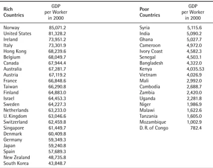
Table A-2.List of Rich and Poor countries, PWT 8.1.

Rich Countries

GDP per Worker

in 2000

Poor Countries

GDP per Worker

in 2000

Norway 85,071.2 Syria 5,115.6

United States 81,328.2 India 5,090.2

Ireland 73,951.2 Ghana 5,027.7

Italy 73,301.9 Cameroon 4,972.0

Hong Kong 68,239.6 Ivory Coast 4,582.3