Residues of Complex Functions with Definite and Infinite Poles on X-axis

(1)

ISSN 1549-3644

Corresponding Author: Abbas Y. Al Bayati, Department of Mathematics, University of Mosul,Iraq

152

Residues of Complex Functions with Definite and Infinite Poles on X-axis

1

Abbas Y. AL-Bayati and

2

Sasan A. Al-Shwani

1

Department Mathematics, Mosul University, Mosul, Iraq

2

Department Mathematics, Kirkuk University, Kirkuk, Iraq

Abstract: Problem statement: One of the most popular areas in the mathematics is the computational complex analysis. In this study several computational complex techniques were investigated and implemented numerically. Objective: This study produced new procedures to compute the residues of complex functions by changing their numerator from a constant number to either even or odd function. Approach: In this project we studied the functions that had finite and infinite poles Zi, i greater than one of order greater or equal one, also we found new relation between residues at the poles Zi and residues at the poles -Zi, i greater than one and we had used these relations to solve improper integrals of this type. The project needed the knowledge of computing the complex improper integrations. Results: Our numerical results in computing the residues for improper integrals of definite and infinite poles on the x-axis were well defined. Conclusion: In this study, we had concluded that the residues of the complex functions had definite and infinite poles of higher order with constant numerator. A general form of residues of these functions of high orders were also investigated.

Key words: Computational complex analysis, finite and infinite poles and residues INTRODUCTION

The residue theorem is one of the main results of complex analysis. It includes Cauchy's theorem and Cauchy's integrals formula as special cases and leads quickly to important applications. In particular it becomes one of the most powerful tools of analysis for evaluation of definite and infinite integrals[3].

If ℜ is the real field and C is the Complex field then consider the following Definitions:

A function f (z) is said to be analytic in a domain D if it has a derivative at every point in the same domain D[4].

A point at which f(z) fails to be analytic is called a singular point of the function f(z) or singularities of the function f(z).There are three type of singular point, Isolated, Removable and Essential[2].

If we can find a positive integer number (m) such

that

(

₀ m

)

z z 0

lim_→ (z−z ) f (z) 0≠ then (z = z0) is called a pole of order (m), as special case if (m = 1) is called simple pole[2].

Let f (z) be analytic inside and on a simple closed curve C. Let (a) and (a+h) be two points inside C ,then the expansion:

2 \ (z a) \ \

f (z) f (a) (z a)f (a) f (a)

2!

−

= + − + +

where, (Z = a+h) is called Taylor's series[5]. MATERIALS AND METHODS

Lemma 1: Let (z0) be a pole of order (m) of a function f(z) then the residues of the functions were given by the formula:

0

m 1

m

0 z z m 1 0

1 d

Res[f , z ] lim [(z z ) f (z)]

(m 1)! dz

−

→ −

= −

−

This was called the (Short-Cut-Method)[3].

Theorem 1: Let f(Z) p(Z) q(Z)= be an analytic function in and on a simple closed curve C except at

)

(Z=±Z₀ then f has a pole of order m (integer number) where p(Z) is constant and the residue at

)

(Z=−Z₀ is harmonic conjugate of the residue at )

(Z=Z₀ i.e,:

0 0

Re s[f , Z ]− =Re s[f , Z ]

(2)

0

0 \ \

0 0

p(Z ) p(Z)

Res[f , Z ]

q (Z ) q (Z )

= = (1)

(because p(Z) is constant) also:

0

0 \ \ \

0 0 0

0

p( Z ) p(Z) p(Z)

Res[f , Z ]

q ( Z ) q (Z ) q (Z )

Res[f , Z ]

−

− = = = − =

− −

−

(2)

Because Z = −Z0 is harmonic conjugate of Z = z0 and there are roots of the function q(Z) therefore:

\ \

0 0

q ( Z )− =−q (Z )

Then we get:

0 0

Re s[f , Z ] Res[f , Z ]− = (3)

Also If Z0 is a pole of order m = 2 then the residue is given by the form:

\ (3)

0 0 0

0 \ \ \ \ 2

0 0

p (Z ) 1 p(Z )q (Z ) Res[f , Z ] 2

q (Z ) 3 (q (Z ))

 

= × − × 

  (4)

P (Z) is constant function then \

p (Z) 0= and

0

p(Z )=p(Z) therefore:

(3) 0

0 \ \ 2

0

1 p(Z) q (Z ) Res[f , Z ] 2

3 (q (Z ))

 

= × − × 

  (5)

Then we evaluate the residue at a pole Z = −Z0 by (Short-Cut-Method):

0

2

0 Z Z 0

d p(Z)

Res[f , Z ] lim (Z Z )

dZ q(Z)

→−

 

− =  + 

  (6)

We expanded the analytic function q(Z) in the bounded region Z+Z0<r by Taylor series expansion:

0

Z Z

2 0

/

0 0 0

2 / / 0 0 d A lim dZ B

A (Z Z ) p(Z)

B q( Z ) (Z Z )q ( Z )

(Z Z )

q ( Z ) .... 2! →−   = _{ }   = + = − + + − + + ₋ ₊ (7) 0

Z Z \ \

\ \ \

0 0

0

d p(Z)

lim

q ( Z ) (Z Z )

dZ

q ( Z ) ...

2! 3! →−     =   − +  ₊ ₋ ₊      (8) Let:

\ \ 0 (3)

0 0

2 (4) 0

0

(Z Z )

U(Z) q ( Z ) q ( Z )

3!

(Z Z )

q ( Z ) ...

3 4 + = − + − + + ₋ ₊ × (9)

Then substituting (9) into (8) we get:

0

\ \

Z Z 2

p (Z) U(Z) p(Z)U (Z)

2lim

U (Z) →−

 ₋ 

=  

  (10)

0

\ \

Z Z 2

p (Z) p(Z) U (Z)

2lim

U(Z) U (Z)

→−

 

=  − 

  (11)

Then by deriving the function (9) for (Z) we get:

\ \ \

\ 0 0 (4)

0 2

(5) 0

0

q ( Z ) (Z Z )

U (Z) q ( Z )

3 6

(Z Z )

q ( Z ) ... 4 5 − + = + − + + ₋ ₊ × (12) 0 0 0 \ \

Z Z 0

\ \

Z Z 0 0

\ \ (3)

Z Z 0 0

lim p (Z) p ( Z ) 0

lim U(Z) U( Z ) q ( Z ).

lim U (Z) U ( Z ) q ( Z ) 3

→− →− →−  = − =  = − = −   = − = − _ (13)

Because p(Z) is constant .Substituting (13) into (12) yields:

(3)

0 0

0 \ \ 2

0

2 p( Z ) q ( Z )

Res[f , Z ]

3 (q ( Z ))

 ₋ ₋ 

− = × 

−

  (14)

Then from Eq. 4 and 14 we have:

0 0

Res[f , Z ]− =Res[f , Z ] (15)

Also If Z = -Z0 is a pole of order (m = 3) then the residue at a pole (Z = Z0) is given by the following formula:

(

)

(

)

(5) 0

0 ₍₃₎ 2

0

( 4 ) 2 0

3 (3)

0

1 p(Z)q (Z )

Re s[f , Z ] 3

10 _q _{(Z )}

1 (q (Z )) p(Z)

8 _q _{(Z )}

(3)

154 Now because p (Z) is constant and

( n ) 0

p (Z )=0 ∀ ≥n 1 and p(Z )0 =p(Z) then by

(short-cut-method) we find the residue at a pole Z = −Z0 of order (m = 3):

0

2

3

0 Z Z 2 0

1 d p(Z)

Res[f , Z ] lim (Z Z )

2 →− dZ q(Z)

 

− =  + 

  (17)

We expand the analytic function q(Z) by Taylor's series valid in the disc Z+Z0<r:

0

2

0 Z Z 2

1 d A

Res[f , Z ] lim

2 →− dZ B

 

− =  _{ } (18)

Where:

A = (Z+Z0)3p(Z) B =

2

\ 0 \ \

0 0 0 0

(Z Z )

q( Z ) (Z Z )q ( Z ) q ( Z ) ...

2

+

− + + − + − +

0

( Z )− is a pole of order (m = 3) then we get:

\ \ \

0 0 0

q( Z )− =q ( Z )− =q ( Z )− =0

But:

(n ) 0

q ( Z )− ≠0 ∀ ≥n 3

Then:

(3) 0 ( 4)

0 0

2 (5) 0

0

(Z Z )

U(Z) q ( Z ) q ( Z )

4

(Z Z )

q ( Z ) ...

4 5 +  = − + − +    + ₋ ₊  ×  (19)

Substituting (19) in Eq. 18 we get the following formula:

0

2

0 Z Z 2

d p(Z)

Res[f , Z ] 3lim

dZ U

→−

 

− = _ _ (20)

0

\ \

Z Z 2

d p (Z)U(Z) p(Z)U (Z)

3lim

dZ U (Z)

→−

 ₋ 

=  

  (21)

0

( 2) (1) \

Z Z 2

(2) (1) (1) \ 2

2 3

U(Z)p (Z) p (Z)U (Z)

3lim

U (Z)

p(Z)U (Z) U (Z)p (Z) (U (Z)) p(Z)

2

U (Z) U (Z)

→−  ₋ =  −   + ₋   (22) Where: 0 0 0 0 0

Z Z 0

\ Z Z

(3)

Z Z 0

\ (4) (5)

0 0 0

\ (4)

Z Z 0

\ \ (5) 0

(6)

0 0

\ \ Z Z

lim p(Z) p( Z )

lim p (Z) 0

lim U(Z) q ( Z )

1 2

U (Z) q ( Z ) (Z Z )q ( Z ) ....

4 4 5

1

lim U (Z) q ( Z )

4 2

U (Z) q ( Z )

4 5 2 3

(Z Z )q ( Z ) ....

4 5 6

lim U (Z)

→− →− →− →− → = − = = − = − + + − + × = − = − + × × ₊ ₋ ₊ × × = (5) 0 1

q ( Z ) 10                   −   (23)

Then substituting the value of (23) into (22) we get the following formula:

(

)

(

)

(5)

0 0

0 (3) 2

0 2 ( 4) 0 0 3 (3) 0

1 p(Z )q (Z )

Re s[f , Z ] 3

10 (q (Z ))

q (Z ) p(Z )

1

8 _{q (Z )}

 − = − − +      (24)

Because q (Z) is even with order (m = 3) then:

(5) (5) (3) (3)

0 0 0 0

q ( Z )− = −q (Z ) and q ( Z )− = −q (Z )

Therefore:

0 0

Re s[f , Z ]− =Res[f , Z ]

In the above manner the procedure can be easily extended for any pole of order (m)[1].

Then by the same way, we can generalize the procedure for any high order poles (m>3).

Theorem 2: Let f (Z) p(Z) q(Z)

= is analytic function in and on a simple closed curve C except at

i

(Z= ±Z , i=1, 2,3,....)if f has poles of order (m>0) where p (Z) is constant then:

i

i 1 i 1

Re s[f , Z ] Res[f , Zi]

∞ ∞

= =

− =

∑

Proof: From above theorem (1) if (Z= ±Z )i is a simple

(4)

1 1

2 2

3 3

n n

Res[f , Z ] Res[f , Z ]

. . .

 − =



− = 



− = 

     

− = _

   

(25)

By addition (25) we get:

1 2 n

Res[f , Z ] Res[f , Z ] ... Res[f , Z ] ...

Res[f , Z ] Res[f , Z ] ... Res[f , Z ] ....

− + − + + − +

= + + + + (26)

Then:

i i

i 1 i 1

∞ ∞

= − = =

∑

(27)

Then the relation is true for all (m>1). Theorem 3: Let f (Z) p(Z)

q(Z)

= is analytic function in and on a simple closed curve C except at

i

(Z= ±Z , i=1, 2,3,....)if f has poles of order (m>0) where p (Z) is constant then:

C

p ( Z )

d Z z e r o

q ( Z ) =

∫

Proof: For all order m>0, we know that:

i i 1

C

p(Z)

dZ 2 i Res[f , Z ]

q(Z)

∞

=

= π

∑

±

∫

(28)

But:

i i i

i 1 i 1 i 1

Res[f , Z ] Res[f , Z ] Res[f , Z ]

∞ ∞ ∞

= = =

± = − +

∑

(29)

By theorem 2 we have:

i i

i 1 i 1

∞ ∞

= =

− =

∑

(30)

Then:

i i 1

Res[f , Z ] zero ∞

= ± =

∑

#

RESULTS

For computing the residues for improper functions of definite poles on x-axis let us consider the following example.

Example 1: Evaluate the following integral:

2 5 2 6

k

dx

(x 4) (x 1)

∞

−∞

∫

− −

where, k is constant. Solution: We know that:

R R

2 5 2 6 2 5 2 6

R

k k

dx lim dZ

(x 4) (x 1) (Z 4) (Z 1)

∞

→∞

−∞ −

=

− − − −

∫

By CPV and on (x-axis).

The function f (Z) ₂ ₅k ₂ ₆

(Z 4) (Z 1)

=

− − has 4th poles

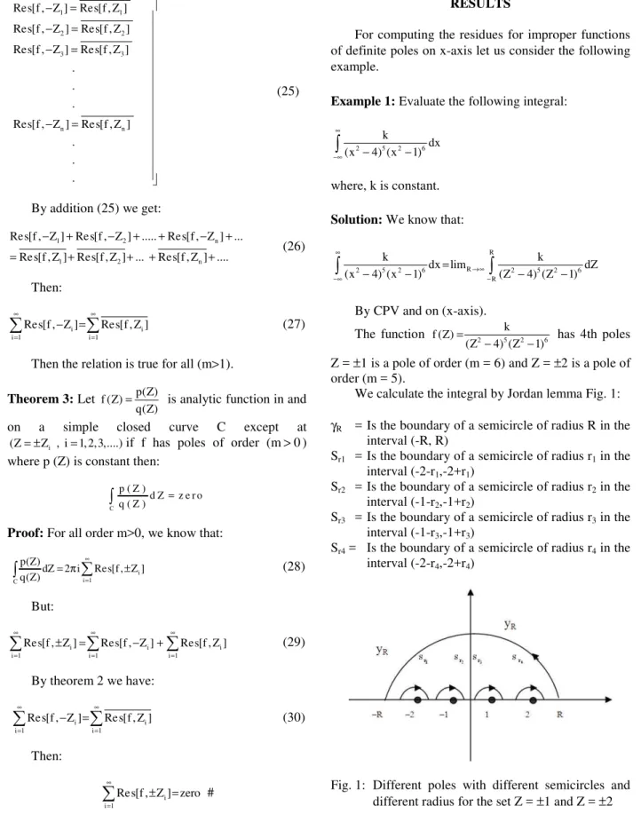
Z = ±1 is a pole of order (m = 6) and Z = ±2 is a pole of order (m = 5).

We calculate the integral by Jordan lemma Fig. 1: γR = Is the boundary of a semicircle of radius R in the

interval (-R, R)

Sr1 = Is the boundary of a semicircle of radius r1 in the interval (-2-r1,-2+r1)

(5)

156 where, R→∞ and ri→ 0, I = 1, 2, 3, 4

Then by Jordan lemma we have:

i

r1 r2 r3 r4 R R

R r 0

R S S S S

lim f (Z) dZ lim ( )f (Z) dZ;

i 1, 2,3, 4

→∞ →

− γ

= + + + +

=

∫

∫ ∫ ∫ ∫ ∫

Where:

R

r1

r3

r4

S

f (Z)dZ 0 as R

f (Z)dZ i Res[f , 2]

f (Z)dZ i Res[f ,1]

γ

= → ∞

= π − = π − = π = π

∫

By new relation we get:

Res[f , 1] Res[f ,1] , Res[f , 2] Res[f , 2]− = − =

We evaluate the residue at Z = 2 (of order m = 5) by the new procedure where:

2 5 2 6

p(Z) k ; q(Z) (Z= = −4) (Z −1)

Then:

(9) (6) (8)

(5) 2 (5) 3

(7) 2 (6) 2 (7)

(5) 3 (5) 4

(6) 4 (5) 5

1 q (2)p(2) 1 q (2)q (2)p(2)

Res[f ,2] 5

126 (q (2)) 42 (q (2))

(1 21 q (2)) p(2) (1 6 q (2)) q (2)p(2)

6 36

(q (2)) (q (2))

(1 6 q (2)) p(2) 24

(q (2)) 

= × × + ×



× ×

+ × − ×



×

+ × 



Substituting the following values in above equation:

( 5 ) ( 6 ) ( 7 ) ( 8 ) ( 9 )

p ( 2 ) k

q ( 2 ) 8 9 5 7 9 5 2 0

q ( 2 ) 4 .9 7 1 7

q ( 2 ) 1 .4 7 8 2

q ( 2 ) 3 .0 6 1 9

q ( 2 ) 4 .8 6 8 9

= = = = = =

We get:

Res[f , 2] 5k [4.8= × +5.04+4.08−2.61 1.85]+ =65.8k

k is a constant. Then we get:

Res[f , 2] Res[f , 2]− = =−65.8 k

Also by the same procedure we get:

Res[f , 1] Res[f ,1]− = =−Res[f ,1]

Therefore:

f (Z) dZ (65.8k 65.8k Res[f ,1] Res[f , 1]) i 0

∞

−∞

= − + + − π =

∫

For computing the residues for improper functions of infinite pole on x-axis let us consider the following example.

Example 2: Evaluate the following integral:

3

k dx

(cos x)

2 ∞

−∞

∫

π

where, k is a constant. Solution: By C.P.V:

R R

3 _R 3

k k

dx lim dx

(cos x) (cos x)

2 2

∞

→∞

−∞ −

=

π π

∫

R R

3 3

R R

k k

dx dZ

(cos x) (cos Z)

2 2

− −

=

π π

∫

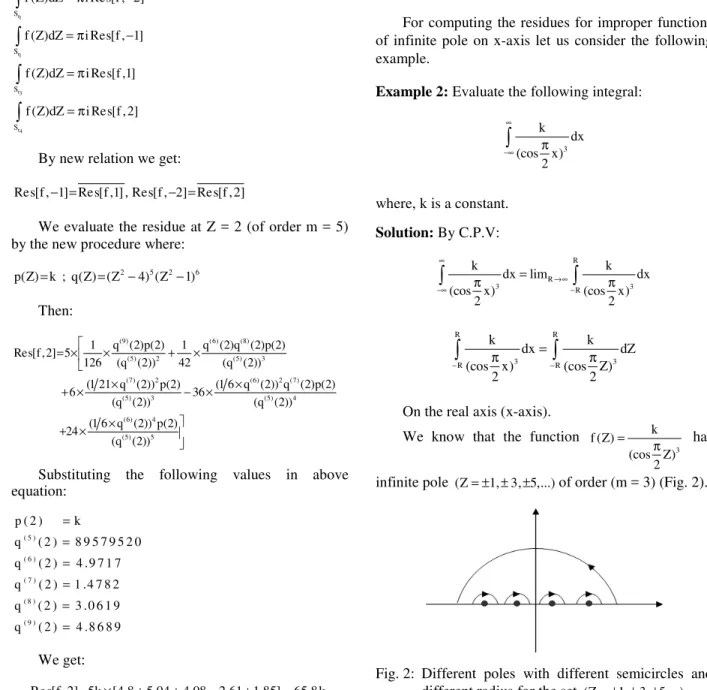
On the real axis (x-axis). We know that the function

3

k f (Z)

(cos Z)

2

= _π has

infinite pole (Z= ± ± ±1, 3, 5,...)of order (m = 3) (Fig. 2).

(6)

γR = The boundary of a semicircle of radius R in the interval (-R, R)

1

r

s = The boundary of a semicircle of radius r1 in the interval (1-r1,1+r1)

Sr−1 = The boundary of a semicircle of radius r−1 in the interval (-1-r-1,-1+r-1)

. . . .

n

r

s = The boundary of a semicircle of radius rn in the interval (±n-r1, ±n+r1) where n is odd number where, R→∞ and ri→ 0, I = ±1, ±2, ±3, ….

r1 r1 rn

R

R S S S

f (Z) dZ f (Z) dZ f (Z) dZ ... f (Z) dZ ...

−

= + + + +

∫

Where:

r1

S

f (Z)dZ=πi Re s[f ,1]

∫

r 1

S

−

=π −

∫

r3

S

f (Z)dZ=πi Res[f ,3]

∫

r 3

S

−

=π −

∫

. .

r n

S

f (Z)dZ i Re s[f , n]

±

= π ±

∫

; n = 5, 7

We find residue at (Z = 1) by using equation then:

(5) (4) 2

(3) 2 3 3

1 p(1) q (1) 1 (q (1)) p(1)

Res[f ,1] 3

10 (q (1)) 8 (q (1))

 

= × − × + × 

 

When:

3

p(Z) k ,q(Z) (cos( Z))

2

π

= =

Then we get:

3 5

(3) 3 (4) (5) 12

p(1) k ; q (1) ; q (1) 0 ; q (1)

4 16

π π

= = = =

Therefore:

3

6

12

k ( )

1 ₁₆ 3 4k 2k

Res[f ,1] 3

9

10 ₍ ₎ 10 3 5

16

 

× π

   

= × − × = − _ _= −

π π

 

 _π 

 

k is a constant. Then by new relation we get:

2k Re s[f , 1] Re s[f ,1]

5

− = =

π

Also by the same procedure we get:

2k Res[f ,3]

5

= π;

2k Re s[f , 3] Re s[f ,3]

5

− = = −

π

. . .

Then we get the general solution:

i 2k

Res[f , n] ( 1) 5

= − × π

where, n = 1 ,3 ,5 ,… (n is pole of order m = 3) and i = 1, 2, 3….

By new relation we get:

i 1 2k

Res[f , n] Re s[f , n] ( 1)

5 +

− = = − ×

π

Then:

R

3 n 2 i 1 R

i i 1 i 1

3

k

dZ ( Res[f , n] Res[f , n]) , i 1, 2,3,...

cos( Z) 2

2k

( ( 1) ( 1) ) Zero

5

k

dx Zero

(cos x)

2

∞

= − −

∞

+

= ∞

−∞

= + − =

π

= − + − =

π

∴ _π =

∑

∫

∑

∫

DISCUSSION

Since there are a finite number of poles of that lie in the upper half plane, a real numbers can be found such that the poles all lie inside the contour C, which consists of the segment -R < x < R of the x axis together with the upper semicircle of radius R. In this study we have investigated and evaluated definite and indefinite integrals of higher order poles with some computationally complex techniques with an efficient numerical results.

CONCLUSION

(7)

158 poles of higher order with constant numerator and we have find a general form of these residues for functions when we have used these facts to evaluate improper integrals. Also we can able to change numerator of these complex functions from a constant number to either even or odd function.

REFERENCES

1. Mathews H. John, 1997. Complex analysis for mathematics and engineering. Jones and Bartlett Publishers International, Barb House, Barb Mews, London W6 7PA, UK., pp: 244-260.

2. Donald H. Trahan, 1965. A new approach to integration for functions of a complex variable. Math. Mag., 38: 132-140.

3. John B. Reade, 2003. Calculus with Complex Numbers. Taylor and Francis is an imprint of the Taylor and Francis Group, ISBN: 041530847X, pp: 100.

4. Stefan, B., 1953. A theorem of green's type for functions of two complex variable. Proc. Am.

Math. Soc., 4: 102-109.

http://www.jstor.org/pss/2032207