www.nonlin-processes-geophys.net/17/499/2010/ doi:10.5194/npg-17-499-2010
© Author(s) 2010. CC Attribution 3.0 License.
in Geophysics
Complex behaviour and predictability of the European
dry spell regimes
X. Lana1, M. D. Mart´ınez2, C. Serra1, and A. Burgue ˜no3
1Departament de F´ısica i Enginyeria Nuclear, Universitat Polit`ecnica de Catalunya, Barcelona, Spain 2Departament de F´ısica Aplicada, Universitat Polit`ecnica de Catalunya, Barcelona, Spain
3Departament de Meteorologia i Astronomia, Universitat de Barcelona, Barcelona, Spain
Received: 11 May 2009 – Revised: 15 July 2010 – Accepted: 23 August 2010 – Published: 30 September 2010
Abstract. The complex spatial and temporal characteristics
of European dry spell lengths, DSL, (sequences of consec-utive days with rainfall amount below a certain threshold) and their randomness and predictive instability are analysed from daily pluviometric series recorded at 267 rain gauges along the second half of the 20th century. DSL are ob-tained by considering four thresholds, R0, of 0.1, 1.0, 5.0 and 10.0 mm/day. A proper quantification of the complexity, randomness and predictive instability of the different DSL regimes in Europe is achieved on the basis of fractal analyses and dynamic system theory, including the reconstruction the-orem. First, the concept of lacunarity is applied to the series of daily rainfall, and the lacunarity curves are well fitted to Cantor and random Cantor sets. Second, the rescaled analy-sis reveals that randomness, peranaly-sistence and anti-peranaly-sistence are present on the European DSL series. Third, the complex-ity of the physical process governing the DSL series is quan-tified by the minimum number of nonlinear equations deter-mined by the correlation dimension. And fourth, the loss of memory of the physical process, which is one of the reasons for the complex predictability, is characterized by the val-ues of the Kolmogorov entropy, and the predictive instability is directly associated with positive Lyapunov exponents. In this way, new bases for a better prediction of DSLs in Europe, sometimes leading to drought episodes, are established. Con-cretely, three predictive strategies are proposed in Sect. 5. It is worth mentioning that the spatial distribution of all fractal parameters does not solely depend on latitude and longitude but also reflects the effects of orography, continental climate or vicinity to the Atlantic and Arctic Oceans and Mediter-ranean Sea.
Correspondence to:X. Lana ([email protected])
1 Introduction
As in many other fields of Geosciences, fractal concepts are very useful for a better knowledge of the physical laws governing the complex natural processes of the pluviomet-ric regimes and their time predictability. The applicability of these physical laws (differential equations of the atmo-spheric dynamics) is limited by several factors such as their intrinsic complexity, the necessity of reliable data (empirical initial conditions free of errors) to solve the equations, and the effects of a complex topography. In this paper, the fractal analysis is constrained to a particular aspect of a pluviometric regime: the dry spell lengths, DSL, which can be defined as the number of consecutive days with rain amounts lowering a certain thresholdR0(mm/day).
The fractal nature of rainfall processes is an accepted fact, confirmed by numerous studies along the last decades. It can be cited Lovejoy and Mandelbrot (1985), Rodr´ıguez-Iturbe et al. (1989), Olsson et al. (1993), Hubert et al. (1993), Tessier et al. (1996), Harris et al. (1996), Veneziano et al. (1996), Svensson et al. (1996), Lima and Grassman (1999), Maz-zarella (1999), MazMaz-zarella and Tranfaglia (2000), Sivaku-mar (2001a, b), SivakuSivaku-mar et al. (2001), Salas et al. (2005) and Mart´ınez et al. (2007a), among many others. Multifrac-tality, chaotic behaviour, time persistence and predictability have been concepts considered by these authors and many variables closely related to rainfall regimes have been analy-sed. Rain intensity, annual amounts, precipitation linked to convective storms, rain gauge network design and episodes of dry spell lengths are some illustrative examples.
of the DSL series, necessary for a better prediction of drought periods, are not so common in the scientific literature. These analyses of predictability should include estimation of pos-sible random components, complexity of the physical mech-anisms generating the DSL episodes, predictive instability of the equations governing the process, and qualification of chaotic behaviour.
The analysis developed in this study is based on the non-linear character of the DSL series and it consists of four steps involving lacunarity, rescaled analysis, the reconstruc-tion theorem and predictive instability. The main objec-tive is to analyse spatial and temporal fractal patterns of the dry spell regime in Europe, which cannot be described by means of statistical tools, as those used, for instance, by Lana et al. (2004, 2006), Burgue˜no et al. (2005), Mart´ınez et al. (2007b), who made use of statistical distributions, re-turn periods and spectral analyses for studying the dry spell behaviour of NE Spain and the Iberian Peninsula.
A similar analysis was performed by Martinez et al. (2007a) for DSL series on the Iberian Peninsula. The present paper should not be considered as a simple exten-sion to a broader area. First, an interpretation of the la-cunarity in terms of Cantor and random Cantor sets is for the first time successfully attempted now. Second, results concerning rescaled analysis and predictive instability (Lya-punov exponents) for the Iberian Peninsula can be compared now with those obtained for the rest of Europe. Third, the analyses based on the reconstruction theorem, not applied by Mart´ınez et al. (2007a), are now developed for the European database. In addition, the concept of Kaplan-York dimension is used also for the first time to characterise other aspects of the predictive instability for European DSL series. In this way, common patterns and outstanding differences on the dry spell regimes throughout Europe would be manifested.
The contents of the paper are arranged as follows. Col-lected database and methodology are introduced in Sects. 2 and 3, respectively. Section 4 is devoted to introduce the main concepts, basic formulations and results concerning la-cunarity, rescaled analysis and reconstruction theorem (com-plexity and predictive instability). The most relevant re-sults and conclusions regarding the fractal analysis of DSL regimes in Europe are summarised in Sect. 5.
2 Databases
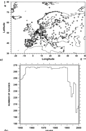
The database consists of 267 time series of daily rainfall records corresponding to European rain gauges. These time series were previously compiled, and their quality and ho-mogeneity checked, by Klein Tank et al. (2002) and Wi-jngaard et al. (2003). These data series are available at http://eca.knmi.nl. Some of the Spanish data come from the Agencia Estatal de Meteorolog´ıa(Spanish Ministry of Envi-ronment) and similar homogeneity and quality controls were applied (Lana et al., 2006). Figure 1a depicts the spatial distribution of these rain gauges. It can be observed that
(a)
AR
-20 -10 0 10 20 30 40 50 60
Longitude 30
40 50 60 70 80
La
titu
de
N
E
(b)
1950 1960 1970 1980 1990 2000
YEARS 180
190 200 210 220 230 240 250 260 270
NUM
BE
R O
F
G
AUG
E
S
Fig. 1. (a)Spatial distribution of the 267 rain gauges in Europe.
(b)Number of available records per year along the recording period.
3 Methodology
The concept of lacunarity introduced by Mandelbrot (1982), which can be interpreted as a measure of clustering of gap sizes in data series, is applied to the series of daily rainfall. Given that the introduction of thresholds is needed for defin-ing “gaps” in these series, lacunarity curves are computed for four thresholds,R0, of 0.1, 1.0, 5.0 and 10.0 mm/day. These same levels are considered to derive four different DSL se-ries for every rain gauge. Lacunarities are then computed by using moving windows of increasing length,r, from 1 to 100 days, thus covering different time scales as days, weeks, months and seasons. As shown later, every lacunarity curve is well described for every rain gauge by two power laws with exponents and changing points depending onR0. Ad-ditionally, in agreement with the basic lacunarity concept (a cluster measure) and the intrinsic behaviour of DSL (lengths increasing with the threshold), it is convenient to check that lacunarity values increase systematically withR0. In addi-tion, the best fit of empirical to synthetic lacunarities gen-erated by Cantor or random Cantor sets is determined by comparing the corresponding misfits. It is worth mentioning that empirical curves reproduced by Cantor sets could repre-sent pluviometric regimes governed by relevant deterministic mechanisms, without excluding certain random components. On the contrary, lacunarities governed by random Cantor sets should be related to pluviometric regimes with very relevant random components. A deterministic example could be the Devil’s staircase model (Fedder, 1988), which is defined as the cumulative Cantor set. Then, for instance, a Cantor set can reproduce the sediment deposition rate paradox, and a Devil’s staircase a stratigraphic thickness sequence (Korvin, 1992). An example of random behaviour is found in the anal-ysis of the monthly North Atlantic Oscillation, NAO, index, where lacunarity curves are well reproduced by a random Cantor set (Mart´ınez et al., 2010).
Additional information regarding the deterministic or ran-dom character of a pluviometric regime could be obtained through the rescaled analysis (Fedder, 1988; Korvin, 1992; Turcotte, 1997), which is applied to the DSL series derived for the different levelsR0. The interpretation of the Hurst exponent,H, provides additional details which reinforce the deterministic or random character of the series analysed. It should be remembered that H close to 0.5 is a clear sign of randomness. On the contrary, H well above 0.5 sug-gests persistence (time trends on previous DSL series con-tribute to DSL prediction) and H well below 0.5 suggests anti-persistence (an average of all previous DSL values tributes to DSL prediction). Then, Hurst exponents con-tribute to a better knowledge of the time behaviour of the dry spell lengths, a very relevant question for assessing hazards concerning water resources and supplies.
Beside lacunarity and rescaled analyses, which quantify gap clustering and randomness versus predictability respec-tively, an additional insight into the characterization of the
dynamical system governing the dry spell time sequence and its predictability is achieved by means of the reconstruction theorem (Grassberger and Procaccia, 1983a; Diks, 1999). Three main parameters are derived from this reconstruction process. First, the correlation dimension, µ∗, can be esti-mated from the analysis of the correlation integral curves (Grassberger and Procaccia, 1983a). This parameter repre-sents the minimum number of nonlinear equations needed for describing the physical mechanism. Second, the Kol-mogorov entropy,κ, is also determined from the same cor-relation curves (Grassberger and Procaccia, 1983b; Cohen and Procaccia, 1983). It represents the loss of memory of the physical process and it could be taken to some extent as a reference for the number of consecutive dry spell lengths to be considered in autoregressive predictive processes. The reconstruction process of the DSL series, for every levelR0 and rain gauge, is repeated by successively increasing dimen-sionm. This process can be shortened and automated under some conditions developed in the present manuscript. A fast automated method for computingκ is proposed and µ∗ is assumed to be the asymptotic value of the slope of the corre-lation integral curve for a high enough reconstruction dimen-sionmof the DSL series. And third, the Lyapunov exponents (Turcotte, 1997) for a reconstruction dimension m, which quantify the degree of predictive instability of the DSL series, are computed by following an algorithm proposed by Eck-mann et al. (1986) and Stoop and Meier (1988). Addition-ally, the Kaplan-Yorke dimension (Kaplan and Yorke, 1979; Grassberger et al., 1991; Diks, 1999) is evaluated taking into account all Lyapunov exponents for every DSL series. Then, the fractal dimension of the strange attractor representing the dynamical system governing DSL can be quantified.
4 Formulation and results
4.1 Lacunarity
The lacunarity is a way of quantifying the distribution of gap sizes within a set of data (Mandelbrot, 1982). It also repre-sents the measure of the failure of a fractal to be transitionally invariant and plays a relevant role in the study of critical phe-nomena. Additionally, several fractal sets with the same frac-tal dimension can be distinguished by their lacunarities, due to their different gap distribution. Large lacunarities imply large gaps and clumping of points, whereas small lacunarities suggest a rather uniform distribution of small gaps. Several illustrative examples can be found in Turcotte (1997), where quite uniform and clumped distributions are related to small and high lacunarities, respectively. Other examples of lacu-narity are those corresponding to series generated by Cantor and random Cantor sets.
be found in Mazzarella (1999) and Lana et al. (2005), respec-tively. Very briefly, referring to the daily rainfall series, the more isolated the clusters of rainy days, the smaller the value ofD. Thus, small values ofDshould be related to high val-ues of lacunarityL. On the contrary, high values of D should represent quite uniformly distributed consecutive rainy days, only separated by short gaps, which would correspond to low values ofL.
At the present application, lacunarity represents a measure of the distribution of segments, defined as the number of con-secutive days with rain amounts equalling or exceeding some threshold valuesR0, and gaps, introduced as the number of consecutive days with rain amounts belowR0. The proba-bility of detecting s segments within a moving window of lengthr(in days) is given by
p(s,r)=n(s,r)/N (r) (1)
whereN (r)is the total number of possible windows of length
r, that isN (r)=ℓ−r+1, withℓthe whole number of record-ing days.n(s,r)is the number of moving windows of length
rcontaining s segments. Finally, the lacunarity, as a function of the segment length,r, is defined as
L(r)= M2(r)
[M1(r)]2
(2) with
M1(r)=
r X
s=1
s·p(s,r); M2(r)=
r X
s=1
s2·p(s,r) (3)
the first and second order moments ofr.
The evolution of the lacunarity for the 267 series is analy-sed by means of moving windows of lengthr ranging from 1 to 100 days, which is equivalent to consider short (daily), medium (monthly) and long (seasonal) scales.
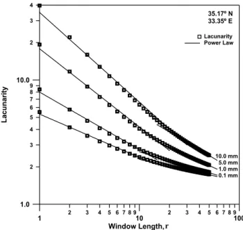
Figure 2 depicts an example of the evolution ofL(r) at a particular rain gauge for the four levelsR0. As expected from the concept of lacunarity and Eqs. (1)–(3),L(r)tends to 1.0 forr tending to∞and the lacunarity increases sys-tematically with the thresholdR0. Moreover, the evolution ofL(r) withr can be analytically described by two power laws for everyR0
L(r)=α1·rβ1; r=1,...,rc (4)
L(r)=α2·rβ2; r=rc,...,ℓ (5)
with parameters (α1,β1) changing to (α2,β2) for a critical window lengthrc. Parametersα1,β1,α2andβ2of the power laws (4a, b) are determined by linear regression on a log-log scale. The critical valuerc is the value leading to the best square regression coefficient for segments within intervals [1−rc] and [rc−ℓ]. A systematic analysis of the 267 time series for the four threshold levels permits to ascertain that all lacunarity curves fulfil Eqs. (4) and (5). Given that the
2 3 4 5 6 7 8 9 2 3 4 5 6 7 8 9
1 10 100
Window Length, s 2
3 4 5 6 7 8 9 2 3 4
1.0 10.0
Lacun
a
rity
10.0 mm 5.0 mm 1.0 mm 0.1 mm 35.17º N 33.35º E
Lacunarity Power Law
r
Fig. 2. An example of lacunarity curves for a daily rainfall series
and the four thresholds (0.1, 1.0, 5.0 and 10.0 mm/day).
most relevant changes in lacunarity are always detected be-fore the critical valuerc, Fig. 3 represents the geographical distribution of parametersα1andβ2and critical lengthsrc, for the four thresholdsR0.
Maps ofα1(Fig. 3a) represent the lacunarity at daily scale, asL(1) is equal toα1. For the first three levelsR0, it can be observed a northwest-southeast gradient ofα1in the Iberian Peninsula and Eastern Mediterranean. The highest lacunari-ties are reached in the south of the Iberian Peninsula. The rest of Europe, except the Eastern Mediterranean, is characterised by an almost constant value ofα1. Some signs suggesting a more complex spatial distribution for 5.0 mm/day are con-firmed in the 10.0 mm/day map, with outstanding lacunarities in Eastern Europe and latitudes north of 60◦N. High lacunar-ities are still observed in the Southern Iberian Peninsula for 10.0 mm/day map. Maps of parameterβ1(Fig. 3b) describe the spatial distribution of the power decay of lacunarity when increasing moving window length r (days). It is relevant that the fastest decay of lacunarity is reached for some areas faced to the Atlantic Ocean (West of the Iberian Peninsula and Scandinavia for instance) and close to the Alps, what-ever the levelR0.
3
-20 -10 0 10 20 30 40
LONGITUDE 35
45 55 65 75
LAT
ITUDE
0.0 2.0 4.0 6.0 8.0 10.0 12.0
1(1.0 mm) N
E
-20 -10 0 10 20 30 40
LONGITUDE 35
45 55 65 75
LAT
ITUDE
0.0 2.0 4.0 6.0 8.0 10.0
1(0.1 mm) E N
-20 -10 0 10 20 30 40
LONGITUDE 35
45 55 65 75
LAT
ITUDE
0.0 10.0 20.0 30.0 40.0 50.0
1(10.0 mm) N
E
-20 -10 0 10 20 30 40
LONGITUDE 35
45 55 65 75
LAT
ITUDE
0.0 5.0 10.0 15.0 20.0 25.0 30.0
1(5.0 mm) N
E
-20 -10 0 10 20 30 40
LONGITUDE 35
45 55 65 75
LAT
ITUDE
-0.6 -0.5 -0.4 -0.3 -0.2 -0.1 0.0
1(0.1 mm) N
E
-20 -10 0 10 20 30 40
LONGITUDE 35
45 55 65 75
LAT
ITUDE
-0.6 -0.5 -0.4 -0.3 -0.2 -0.1
1(1.0 mm) N
E -20 -10 0LONGITUDE10 20 30 40
35 45 55 65 75
LAT
ITUDE
-0.8 -0.7 -0.6 -0.5 -0.4 -0.3
1(10.0 mm) N
E
-20 -10 0 10 20 30 40
LONGITUDE 35
45 55 65 75
LAT
ITUDE
-0.7 -0.6 -0.5 -0.4 -0.3 -0.2
1(5.0 mm) N
E
(a) (b)
(c)
-20 -10 0 10 20 30 40
LONGITUDE 35
45 55 65 75
LAT
ITUDE
0.0 10.0 20.0 30.0 40.0
c(0.1 mm)
S
N
E -20 -10 0LONGITUDE10 20 30 40
35 45 55 65 75
LAT
ITUDE
0.0 10.0 20.0 30.0 40.0 50.0
c(1.0 mm)
S
N
E
-20 -10 0 10 20 30 40
LONGITUDE 35
45 55 65 75
LAT
ITUDE
0.0 10.0 20.0 30.0 40.0 50.0
c(5.0 mm)
S
N
E -20 -10 0LONGITUDE10 20 30 40
35 45 55 65 75
LAT
ITUDE
0.0 10.0 20.0 30.0 40.0 50.0
c(10.0 mm)
S
N
E
rC rC
rC rC
Fig. 3. (a)Spatial distribution of parameterα1in the power law relating lacunarities and moving window lengths, for 0.1, 1.0, 5.0 and
10 mm/day.(b)The same distribution for parameterβ1.(c)Spatial distribution of the critical value,rc, for the same thresholds.
observed, which could be reasonably expected taking into ac-count that gap sizes in rainfall series tend to increase with the threshold levelR0. In short, areas with long-lasting rainfall deficits (high values ofrc) would be characterised by low ab-solute values ofβ1. On the contrary, in areas with short rain-fall deficits (low values ofrc), absolute values ofβ1would be high, and the lacunarity relevantly decreases in a limited range of days. It should be emphasised that in many places
of Europe the decrease of the lacunarity becomes quite irrele-vant forrclonger than 10–20 days, especially for 0.1, 1.0 and 5.0 mm/day, in contrast with other areas where 40–50 days are necessary.
4
-20 -10 0 10 20 30 40 50 60
Longitude 30
40 50 60 70 80
La
ti
tu
de
Cantor Random Cantor 0.1 mm N
E
-20 -10 0 10 20 30 40 50 60
Longitude 30
40 50 60 70 80
La
ti
tu
de
Cantor Random Cantor 5.0 mm N
E
-20 -10 0 10 20 30 40 50 60
Longitude 30
40 50 60 70 80
La
ti
tu
de
Cantor Random Cantor 10.0 mm N
E
-20 -10 0 10 20 30 40 50 60
Longitude 30
40 50 60 70 80
Latitude
Cantor Random Cantor 1.0 mm
E N
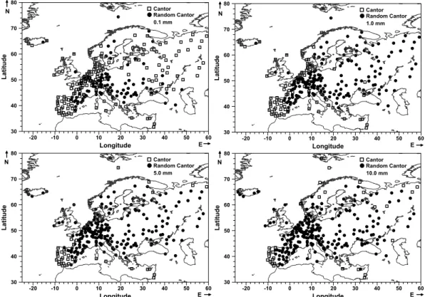
Fig. 4.Spatial distribution of sites where lacunarity curves are best fitted to Cantor (open squares) or random Cantor (solid circles) sets.
generation an element is fragmented into two new pieces and a gap of relative sizeG. If empirical lacunarity curves are well fitted to random Cantor series, there are clear signs of randomness governing the daily rainfall process, especially if this fit is confirmed for all theR0values. Conversely, if empirical lacunarity curves are best fitted to a Cantor set, it can be assumed that a deterministic behaviour is more rele-vant in the rainfall process that a possible background ran-domness. This kind of analysis, discriminating between pure randomness and pure deterministic behaviours, has been re-cently applied to monthly series of the North Atlantic Oscil-lation (NAO) index (Mart´ınez et al., 2010).
Figure 4 shows the spatial distribution of sites where la-cunarity curves are best fitted to random Cantor or Cantor sets. It is observed that a pure single model (either random or deterministic) for all the rainfall series would be an ex-cessively simple description. First, the number of lacunar-ity curves best fitted to a random Cantor model increases withR0. Second, although for 10.0 mm/day many lacunar-ity curves, mostly corresponding to the Atlantic coast of the Iberian Peninsula and to high latitudes, are best fitted to a random Cantor set, a non negligible number of empirical la-cunarities are not well enough fitted to any of the two mo-dels. Table 1 summarises the results of the fits obtained for the different levelsR0. It is observed that the expected value of the relative gap size, G, generating the best fit to deter-ministic/random Cantor lacunarities tends to increase with
R0, in agreement with the increase of empirical lacunarities
Table 1.Average relative gap size,< G >, and standard deviation,
SD(G), of the lacunarity curves for 267 rainfall daily series and four thresholdsR0. Cand RC are the percentage of lacunarity curves
fitted to Cantor and random Cantor sets, respectively. MF designs the ratio of empirical lacunarity curves not well enough fitted to any of the two models.
R0 < G > SD(G) C RC MF
(mm/day) (%) (%) (%) 0.1 0.10 0.05 59.2 40.8 0.0 1.0 0.16 0.04 31.7 68.3 0.0 5.0 0.25 0.04 15.8 84.2 4.5 10.0 0.38 0.08 14.7 85.3 32.1
2 3 4 5 6 7 8 9 2 3 4 5 6 7 8 9 2
100.0 1000.0
Segment Length,
2 3 4 5 6 7 8 9 2 3 4 5 6 7 8 9
1.0 10.0 100.0
R/S
τ ( 0.1 mm ) H = 0.543 0.001 = 0.9972 (56.87º N, 14.80º E)
2 3 4 5 6 7 8 9 2 3 4 5 6 7 8 9 2
10.0 100.0 1000.0
Segment Length,
2 3 4 5 6 7 8 9 2 3 4 5 6 7 8 9
1.0 10.0 100.0
R/
S
τ ( 1.0 mm ) H = 0.505 0.002 = 0.9812
(56.87º N, 14.80º E)
2 3 4 5 6 7 8 9 2 3 4 5 6 7 8 9 2
10.0 100.0 1000.0
Segment Length,
2 3 4 5 6 7 8 9 2 3 4 5 6 7 8 9
1.0 10.0 100.0
R/
S
τ ( 5.0 mm ) H = 0.498 0.001 = 0.9902
(56.87º N, 14.80º E)
2 3 4 5 6 7 8 9 2 3 4 5 6 7 8 9 2
10.0 100.0 1000.0
Segment Length,
2 3 4 5 6 7 8 9 2 3 4 5 6 7 8 9
1.0 10.0 100.0
R/
S
τ ( 10.0 mm ) H = 0.474 0.001 = 0.9692
(56.87 N, 14.80 E)
Fig. 5.An example of rescaled analysis for the DSL series and the four thresholds (0.1, 1.0, 5.0 and 10.0 mm/day).
4.2 Rescaled analysis
The rescaled analysis, and more specifically the Hurst expo-nent (Fedder, 1988; Goltz, 1997), provides us with criteria to qualify the predictability of a complex dynamic system such as the dry spell regime. Applications to a variety of fields in Geology and Geophysics are shown by Korvin (1992) and Turcotte (1997). Some applications in Climatology and more specifically to rainfall regimes can be found in O˜nate (1997), Miranda and Andrade (1999, 2001), Whiting et al. (2003), Miranda et al. (2004) and Mart´ınez et al. (2007a), among others.
The predictability of the DSL series is quantified by inter-preting the meaning of the Hurst exponentH. For every DSL series, mean values and cumulative differences are computed for subsets of DSL series with different number of elements
τ. After that, maximum range,R(τ ), of the integrated signal and standard deviation,s(τ ), for the subsets are computed. If the fractal behaviour exists, the relationship
R(τ )/S(τ )=a·τH (6)
is accomplished. As mentioned in Sect. 3, the value ofH
and its uncertainty are useful tools to quantify the random-ness, persistence or anti-persistence of the physical process governing the sequence of dry spells. The reliability of the estimated values ofH is based on three constraints. First, a low uncertainty onH; second, an acceptable square regres-sion coefficient for the representation of log{R/S}in terms of log(τ); third, the linear evolution of the log-log plot should cover at least two magnitude orders ofτ.
Figure 5 shows an example of rescaled analysis for a rain gauge and the four levels R0. It can be observed that the squared regression coefficient exceeds 0.96 in all cases, the uncertainty onHaffects the second decimal digit and the re-quirement of a minimum of two magnitude orders forτ is also accomplished. Values ofτ less than 10 have not been considered to avoid computational artefacts. This is an ex-ample where the randomness of the physical process govern-ing dry spells would be relevant, as all Hurst exponents are very close to 0.5.
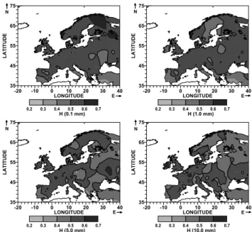
The same procedure for obtaining the Hurst exponentH
throughout Europe for the four thresholds. The thick con-tour line (H= 0.5) delimits areas of persistence and anti-persistence. For 0.1 mm/day, some sites at low latitudes are characterised by anti-persistence, whereasHexceeds 0.5 for the rest of Europe. A quite similar pattern is obtained for 1.0 mm/day, with a nucleus of anti-persistence in the Scan-dinavian Peninsula. The spatial distribution is much more complex for the other two levels. Even though the values of
Hkeep within the same range, a simple geographical delim-itation of areas of persistence and anti-persistence is not evi-dent. Then, Fig. 6 suggests that the same local rainfall regime frequently generates DSL series with predictive characteris-tics varying from persistence to anti-persistence depending on the thresholdR0, as for example, in some areas of Scan-dinavian Peninsula. This is a sign of complexity of the rain-fall regime, and particularly, of the DSL series. This feature is to be confirmed by the reconstruction theorem and related parameters quantifying complexity and predictive instability.
4.3 Reconstruction theorem
The reconstruction theorem (Takens, 1981; Grassberger and Procaccia, 1983a, b) permits a useful analysis of the com-plexity and predictive instability of the rainfall regime and, in particular, of the DSL series. The space of the dynamical system governing the dry spells is reconstructed by generat-ing a setzj of m-dimensional vectors
zj=xj, xj+1,... xj+m−1 j=1,...,n−m+1 (7) beingxj the elements (lengths given in days) of the DSL
se-ries for a givenR0andmthe dimension of the reconstructed space. From the set of vector generated by Eq. (6) the corre-lation function
C(r)= lim
N→∞ 1
N2
N X
i,j=1
Hr−Zi−Zj
(8)
is straightforward to compute, wherer are distances in the m-dimensional space and H{ · } is the Heaviside function. According to Diks (1999),C(r)behaves as
C(r)=Amrµ(m)e−mκ (9)
µ(m) being the correlation dimension, Am the correlation
amplitude andκ the Kolmogorov entropy. It should be re-membered that for a high enough dimensionm, usually de-signed as embedding dimension,dE, µ∗=µ(dE)represents the minimum number of nonlinear equations required to de-scribe the physical system governing the DSL series, andκ
the loss of memory of this system with time. Consequently, both parameters represent an insight into the complexity and predictability of DSL. For instance,κcould help us to select the number of consecutive DSL elements to be considered in an autoregressive process.
-20 -10 0 10 20 30 40
LONGITUDE 35
45 55 65 75
LA
TI
TU
DE
H (0.1 mm)
0.2 0.3 0.4 0.5 0.6 0.7
N
E -20 -10 0LONGITUDE10 20 30 40
35 45 55 65 75
LA
TI
TU
DE
H (1.0 mm)
0.2 0.3 0.4 0.5 0.6 0.7
N
E
-20 -10 0 10 20 30 40
LONGITUDE 35
45 55 65 75
L
A
TI
TU
DE
H (5.0 mm)
0.2 0.3 0.4 0.5 0.6 0.7
N
E -20 -10 0LONGITUDE10 20 30 40
35 45 55 65 75
L
A
TI
TU
DE
H (10.0 mm)
0.2 0.3 0.4 0.5 0.6 0.7
N
E
Fig. 6.Spatial distribution of the Hurst exponent for the four
thres-holds (0.1, 1.0, 5.0 and 10.0 mm/day).
A reiterative search of parameters µ∗ and κ for the 267 daily rainfall records and the four thresholdsR0would be very tedious and time spending. Then, an automated pro-cedure is proposed. If logarithms are taken in Eq. (8) log{C(r)} =log{Am} +µ(m)log(r)−mκ (10)
the slope of the log-log representation is the correlation di-mension,µ(m), for them-dimensional space. The correla-tion curves behave in different ways for three ranges ofr. In the first range ofr, a quite irregular evolution attributable to the lacunarity and an average slope, notably less than that es-timated for the next range ofr, are observed. In the second range, an almost perfect linear evolution of log{C(r)}with log(r) permits to computeµ(m), which will be the highest slope of the three ranges. For the last range, the correlation function saturates to 1.0 and its average slope is again no-tably smaller thanµ(m). Consequently, the largest quotient for finite differences of log{C(r)}and log(r) for moving win-dows along the correlation curves has to be a good approach of µ(m). Then, if the correlation curves are calculated for a high dimensionm, a stationary value of the correlation di-mension,µ∗, is reasonably determined.
Another aspect is the estimation of the Kolmogorov en-tropy,κ. Coming back to Eq. (9), the slope of the evolution of
α(m)=log{Am} −mκ (11)
2 4 6 8 2 4
1E+0 1E+1
r 2
4 6 8 2 4 6 8 2 4 6 8 2
1E-3 1E-2 1E-1 1E+0
C(r)
m = 2 - 10, 13, 15, 17, 19 56.9º N, 14.8º E
(m = 2)
(m = 19)
Fig. 7. An example of the correlation function (dashed lines) of a
DSL series and linear evolution on a log-log scale (solid line) for m ranging from 2 to 19.
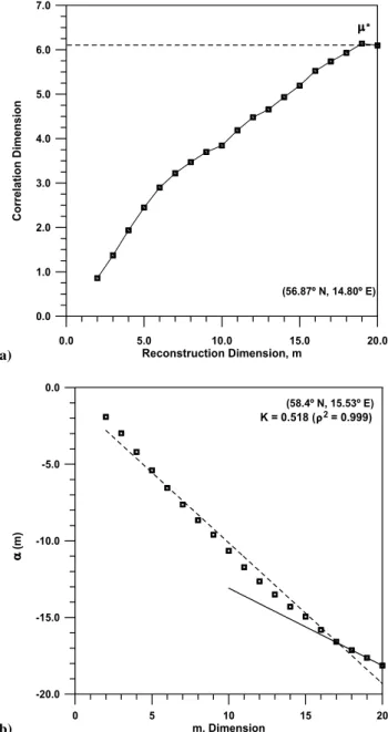
An example of the assumed behaviour for theC(r)curves of DSL is shown in Fig. 7. The effects of lacunarity are de-tectable from a dimensionmequal to 4 or 5 and saturation to 1.0 is always present, whatever the dimensionm. At the same time, the largest slopes,µ(m), indicated by solid lines, tend asymptotically towards a constant value,µ∗.
Figure 8 depicts an example of the evolution of the correla-tion dimension and the determinacorrela-tion of the Kolmogorov en-tropy. Remembering the meaning of the correlation dimen-sion (Diks, 1999), it would be necessary at least six nonlin-ear equations to describe the physical process generating the DSL series. An attempt to quantify more accuratelyµ∗by exploring reconstruction dimensionsmhigher than 20 would not be advisable. Three issues need to be discussed. First, the constraintdE>2µ∗+1 for a right quantification ofµ∗ (Mart´ınez et al., 2010) is still fulfilled, taking into account that the highest exploring dimension is 20 andµ∗ is very close to 6.0. Second, as can be observed in the example of Fig. 7, the range of r for which there is a linear relationship between log{C(r)}and log(r) diminishes withmdue to the above mentioned effects of lacunarity and saturation. In con-sequence, additional estimations ofµcould not be extremely accurate. Third, asµ∗is only a lower bound to the required number of nonlinear equations, and considering the evolution ofµfor high values ofm, a substantial change onµ∗would be unlikely. Finally, some fluctuations in the evolution ofµ
towardsµ∗would be attributable to errors on the slope of the linear relationship between log{C(r)}and log(r). These er-rors could be attributable to missing DSLs or departures of
C(r)from the power law given by Eq. (8). Remembering
(a)
0.0 5.0 10.0 15.0 20.0
Reconstruction Dimension, m
0.0 1.0 2.0 3.0 4.0 5.0 6.0 7.0
Correla
tion D
im
e
nsion
*
(56.87º N, 14.80º E)
(b)
0 5 10 15 20
m, Dimension
-20.0 -15.0 -10.0 -5.0 0.0
(m
)
K = 0.518 ( = 0.999)2 (58.4º N, 15.53º E)
Fig. 8. (a)An example of the evolution of the correlation
dimen-sion,µ(m) towards a stationary value,µ∗. (b)An example of the right (solid line) and wrong (dashed line) computation of the Kol-mogorov entropy.
how lack of data is managed (Sect. 2), it should be accepted that discarded dry spells might be a cause for these fluctua-tions.
With respect to the estimation of the Kolmogorov entropy, it is relevant to observe that whereas entropy close to 0.5 is obtained by consideringmranging from 16 to 20, a linear fit for the whole range ofm(from 2 to 20) would lead to a wrong determination ofκ, close to 0.9. For a right computation,Am
must be very close toAm+1, and the linear fit be almost
6
-20 -10 0 10 20 30 40
LONGITUDE 35
45 55 65 75
LA
TITU
DE
3.0 4.0 5.0 6.0 7.0 8.0
* (0.1 mm)
N
E
-20 -10 0 10 20 30 40
LONGITUDE 35
45 55 65 75
LA
TITU
DE
3.0 4.0 5.0 6.0 7.0 8.0
* (1.0 mm)
N
E
-20 -10 0 10 20 30 40
LONGITUDE 35
45 55 65 75
LA
TITU
DE
3.0 4.0 5.0 6.0 7.0 8.0
* (5.0 mm)
N
E -20 -10 0LONGITUDE10 20 30 40
35 45 55 65 75
LA
TITU
DE
3.0 4.0 5.0 6.0 7.0 8.0
* (10.0 mm)
N
E
Fig. 9.Spatial distribution of the asymptotic values of the
correla-tion dimension for thresholds of 0.1, 1.0, 5.0 and 10.0 mm/day.
linear fit is deceptive and the Kolmogorov entropy is over-valued. An additional issue to be considered is the high di-mensionmneeded to obtain asymptotic values of the correla-tion dimension and a right estimacorrela-tion ofκ. This fact is com-mon to all series and levelsR0. This necessity for a high re-construction dimension also manifests the complexity of the DSL predictive processes. If the right reconstruction of DSL series was achieved with low dimensions, a dry spell episode would solely depend on a few previous episodes and, pos-sibly, a quite simple autoregressive process could be a good predictive tool. Nevertheless, the real physical process gov-erning DSL series (differential equations of the atmospheric dynamics and effects of the topography, vicinity to oceans, etc) is much more complex. Even higher complexities in the atmosphere-ocean coupled dynamics have been found in the analysis of the NAO index (Mart´ınez et al., 2010).
Figure 9 depicts the spatial distribution ofµ∗ for thres-holds of 0.1, 1.0, 5.0 and 10.0 mm/day. According to Ru-elle (1990), the stationary value of the correlation dimension accomplishesµ∗<2loge(M), beingMthe number of DSL
elements for a series. The values ofµ∗ for all thresholds
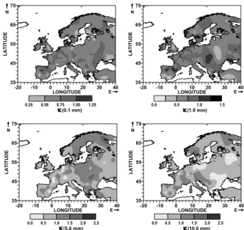
R0vary within a wide range, from 3 to 8. Their spatial pat-terns also change with the threshold. In consequence, for ev-ery rain gauge, the required minimum number of nonlinear equations changes withR0. Figure 10 shows that a similar situation is detected for the entropyκ. Besides the range ofκ
increases withR0, spatial patterns change depending on the threshold. Once again, additional complexities appear be-cause the loss of memory of the physical system governing DSL depends on the levelR0and the geographical location of rain gauges. Remembering shortcomings affecting the
es-2
-20 -10 0 10 20 30 40
LONGITUDE 35
45 55 65 75
LAT
ITUD
E
0.25 0.50 0.75 1.00 1.25
(0.1 mm)
N
E -20 -10 0LONGITUDE10 20 30 40
35 45 55 65 75
LAT
ITUD
E
0.0 0.5 1.0 1.5
(1.0 mm)
N
E
-20 -10 0 10 20 30 40
LONGITUDE 35
45 55 65 75
LAT
ITUD
E
0.0 0.5 1.0 1.5 2.0 2.5
(5.0 mm)
N
E -20 -10 0LONGITUDE10 20 30 40
35 45 55 65 75
LAT
ITUD
E
0.0 0.5 1.0 1.5 2.0 2.5
(10.0 mm)
N
E
Fig. 10. Spatial distribution of the Kolmogorov entropy for
thres-holds of 0.1, 1.0, 5.0 and 10.0 mm/day.
timation ofµ∗ andκ, it is obvious that an automated selec-tion of these two parameters is not convenient and a one-by-one revision for every DSL series is advisable.
4.4 Predictive instability
Associated with the reconstruction theorem and recon-structed vectors, the predictive instability is conceptually defined as the effect of an inaccurate starting state z0 on the uncertainty on the statezj, after j-steps of the
dynam-ical system. The validation of this effect could be ad-dressed either to the computation of the largest positive Lyapunov exponent, λmax (the main generator of predic-tive instability), or the evaluation of the m Lyapunov ex-ponents {λmax=λ1> λ2> ... > λm}. With this second
op-tion, Kaplan-Yorke dimensions, DKY, are then determined from the Lyapunov exponents. If the sum of all the Lya-punov exponents is negative, the Kaplan-Yorke dimension is expressed as
DKY=ℓ0+ 1
λℓ0+1
ℓ0
X
j=1
λj (12)
beingℓ0the largest integer for whichλ1+λ2+...+λℓ0>0.
The different states of the reconstructed vectors in the m-dimensional space would generate strange attractors if they could be defined as bounded sets of aperiodic trajectories asymptotically stables and sensitive to initial conditions. The fractal dimension of these strange attractors would be then quantified by the Kaplan-Yorke (or Lyapunov) dimension,
Table 2.Minimum, maximum and expected values and standard deviations of the sum of all Lyapunov exponents,ST, and the Kaplan-Yorke,
DKY, dimension. Range and expected values of the number,NP, of positive Lyapunov exponents are also included.
ST NP DKY
R0(mm/day) Min Max < ST> σ (ST) < NP> Range Min Max < ST> σ (ST)
0.1 –0.99 –0.60 –0.78 0.07 6.7 5–8 12.61 14.08 13.45 0.20 1.0 –0.92 –0.56 –0.79 0.06 6.8 6–7 12.87 14.08 13.42 0.20 5.0 –0.96 –0.49 –0.79 0.07 6.6 5–7 12.89 14.11 13.38 0.21 10.0 –1.21 –0.37 –0.84 0.10 6.6 5–7 10.78 14.40 13.20 0.41
Wolf et al. (1985) proposed an algorithm to compute non-negative Lyapunov exponents, responsible for predictive in-stability. A more sophisticated computational algorithm (Eckmann et al., 1986; Stoop and Meier, 1988) permits to obtain all the Lyapunov exponents for a reconstruction space of dimensionm. The step-by-step detailed procedure of this algorithm can be found in Mart´ınez et al. (2007a). It has to be pointed out that it must be applied for many dimensions
mwith the aim of obtaining a set ofmstationary Lyapunov exponents. As verified by Mart´ınez et al. (2010), it is usual that these stationary values are achieved at values of m less than those corresponding to the embedding dimension,dE, determined in Sect. 4.3.
Figure 11 summarises the spatial distribution of the first positive Lyapunov exponent, which is the main responsi-ble of predictive instability. As for the previous fractal pa-rameters, the spatial patterns are relatively complex because they change withR0. For 0.1 and 1.0 mm/day, the dominant value forλ1is within a narrow range of 0.20–0.25, except for the Southwest of the Iberian Peninsula, Southern Italy and Turkey, where values from 0.30 to 0.35 are reached. These would be areas where uncertainties on starting values could lead to the largest erroneous long-term predictions of DSL at theseR0 levels. On the contrary, the spatial distri-bution for 5.0 and 10.0 mm/day becomes more complex, the South-western Iberian Peninsula, Southern Italy and Turkey still keeping the highest values ofλ1. Considerable values also appear at high latitudes and the spatial heterogeneity in-creases in Central and Western Europe. Then, whereas the predictive instability of DSL does not generally increase with
R0, its spatial distribution becomes more complex. Addition-ally, given that the first Lyapunov exponent is positive for all rain gauges and levels R0, the mechanism governing DSL series has a degree of predictive instability and chaotic be-haviour and it could be assumed as dissipative (Kolmogorov entropy different from zero).
Table 2 lists expected values, standard deviations and ranks of variation of the sum of all Lyapunov exponents,ST, and Kaplan-Yorke dimension,DKY. It can be concluded that slight spatial variation of these parameters exists. Whatever the levelR0, the strange attractors corresponding to every DSL series are characterised by a very similar fractal
dimen-1
-20 -10 0 10 20 30 40
LONGITUDE 35
45 55 65 75
LA
TIT
U
DE
0.15 0.20 0.25 0.30 0.35 0.40
(0.1 mm)1
N
E -20 -10 0LONGITUDE10 20 30 40
35 45 55 65 75
LA
TIT
U
DE
0.15 0.20 0.25 0.30 0.35
(1.0 mm)1
N
E
-20 -10 0 10 20 30 40
LONGITUDE 35
45 55 65 75
LATI
TUDE
0.15 0.20 0.25 0.30
(5.0 mm)1
N
E -20 -10 0LONGITUDE10 20 30 40
35 45 55 65 75
L
A
TI
TUDE
0.10 0.15 0.20 0.25 0.30 0.35
(10.0 mm)1
N
E
Fig. 11.Spatial distribution of the first positive Lyapunov exponent
for thresholds of 0.1, 1.0, 5.0 and 10.0 mm/day.
5 Conclusions
Several concepts of fractal analysis and dynamic system the-ory applied to 267 European daily rainfall series recorded along 50 years, and distinguishing four different thresholds of daily rainfall, have permitted to estimate the most relevant features regarding randomness, predictability and predictive instability of the DSL regime in Europe. The behaviour of a DSL regime is a very relevant feature taking into account that drought periods (long dry spells or successive dry spells of moderate length) could affect water supplies, agriculture, industry and many other human activities.
Dry spell regimes in Europe are characterised by a no-table variety of spatial patterns depending on the threshold
R0. The main features are:
– The lacunarity can be represented by Cantor or random Cantor sets. It is observed that the percentage of la-cunarity curves represented by random Cantor sets in-creases withR0. In spite of this, a non negligible per-centage of DSL series for 10.0 mm/day should be bet-ter represented by other models different than Cantor or random Cantor sets.
– Hurst exponents suggest randomness, persistence or anti-persistence, the most complex spatial distribution ofH corresponding to 5.0 and 10.0 mm/day. In agree-ment with the meaning of the Hurst exponent, autore-gressive processes would be only applicable to DSL se-ries with clear persistence (H well exceeding 0.5). Al-though Europe is characterised by Hurst exponents ex-ceeding 0.5, especially for 0.1 and 1.0 mm/day, values ofH within the 0.6–0.7 interval are not very common. Consequently, a predictive scheme based on time trends (persistence) would not be very efficient, at least from the point of view of the rescaled analysis.
– The minimum number of nonlinear equations (asymp-totic correlation dimension, µ∗) required to describe the physical process governing the DSLs varies from one place to another and with the threshold, and ranges from a relatively simple system of three equations up to a much more complex eight-equation system. An ex-ample of this variability is given by comparing the be-haviour ofµ∗for an area of Western Europe including parts of France, Germany and Belgium. Whereas for 0.1 and 1.0 mm/day the necessary number of nonlinear equations ranges from 7 to 8, it decreases to 5–6 for 5.0 and 10.0 mm/day. A similar decrease of the predictive complexity is detected, for instance, for western Iberian Peninsula.
– Random components disturbing the nonlinear system of equations are notable in all cases taking into account that a high embedding dimensiondEis always necessary to reach stationary values ofµ.
– The loss of memory of the dynamic system governing DSL regimes is quantified by the Kolmogorov entropy,
κ. The values of κ vary within a wider range for 5.0 and 10.0 mm/day than for the lowest thresholds. This is a relevant fact if a prediction is to be attempted in terms of autoregressive processes, because the number of useful consecutive DSLs for the predictive process diminishes whenκ increases.
– The predictive instability is detected for all DSL se-ries and thresholds, with ranges for the first positive Lyapunov exponents (0.15 to 0.40) quite similar for 0.1, 1.0, 5.0 and 10.0 mm/day. Thus, predictive instability is quite similar for all Europe, except for the southwest of the Iberian Peninsula, where Lyapunov exponents reach maxima close to 0.35 whatever the threshold.
– Only the Kaplan-York dimension,DKY, characterising the fractal dimension of the strange attractors governing the successive DSLs, shows a common pattern for all thresholdsR0. This dimension is constrained to a nar-row range from a minimum exceeding 12.0 to a max-imum close to 14.0 and the number of positive Lya-punov exponents is very similar for all gauges and thres-holds. Only for 10.0 mm/day the minimum dimension decreases to 11.0. The high dimensionDKY is a clear sign of complexity. To obtain aperiodic stable trajecto-ries around the attractor describing the physical process it is necessary to generate reconstruction vectorszj of
dimension at least 11 or 12.
A single predictive strategy for all rain gauges and thres-holds has to be discarded given that all fractal parameters depend on the geographic location and the threshold level. It can be assumed that, at local scale, the effects of atmo-spheric dynamics governing the rainfall regime (and dry spell regimes) may be influenced by the orography, continental cli-mate or the vicinity to the Atlantic and Artic Oceans and Mediterranean Sea. Thus, lacunarity, rescaled analysis and reconstruction theorem results at local scale should be taken into account to decide the best predictive strategy.
DSL series with the convenient gap sizeGis a viable alterna-tive when lacunarity is well fitted to Cantor or random Cantor sets.
Acknowledgements. This research was supported by the
Mi-nistry of Science and Technology, Spanish Government, project CGL2008-00869/BTE.
Edited by: Z. Toth
Reviewed by: two anonymous referees
References
Burgue˜no, A., Mart´ınez, M. D., Lana, X., and Serra, C.: Statistical distribution of the daily rainfall regime in Catalonia (NE Spain) for the years 1950–2000, Int. J. Climatol., 25, 1381–1403, 2005. Cohen, A. and Procaccia, I.: Estimation of Kolmogorov entropy from time signals of dissipative and conservative dynamical sys-tems, Phys. Rev. A, 31, 1872–1882, 1983.
Diks, C.: Nonlinear Time Series Analysis. Methods and Applica-tions, in: Nonlinear Time Series and Chaos (4), World Scientific, London, 209 pp., 1999.
Eckmann, J. P., Oliffson, S., Ruelle, D., and Cilliberto, S.: Lya-punov exponents from time series. Phys. Rev. A, 34(6), 4971– 4979, 1986.
Fedder, J.: Fractals, edited by: Plenum, New York USA, 1988. Goltz, Ch.: Fractal and Chaotic properties of Earthquakes, in:
Lec-ture Notes in Earth Sciences, 77, Springer, Berlin, 175 pp., 1997. Grassberger, P. and Procaccia I.: Characterization of strange
attrac-tors, Phys. Rev. Lett., 50, 346–349, 1983a.
Grassberger, P. and Procaccia, I.: Estimation of the Kolmogorov entropy from a chaotic signal, Phys. Rev. A, 28, p. 2591, 1983b. Grassberger, P., Schreiber, T., and Shaffrath, C.: Nonlinear time
sequence analysis, Int. J. Bifurcat. Chaos, 1, 521–547, 1991. Harris, D., Menabde, M., Seed, A., and Austin, G.: Multifractal
characterization of rain fields with a strong orographic influence, J. Geophys. Res., 101, 26405–26414, 1996.
Hubert, P., Tessier, Y., Lovejoy, S., Shertzer, D., Schmitt, F., Ladoy, P., Carbonnel, J. P., Violette, S., and Desurosne, I.: Multifractal and extreme rainfall events, Geophys. Res. Lett., 20(10), 931– 934, 1993.
Kaplan, J. K. and Yorke, J. A.: Chaotic behaviour of multidimen-sional difference equations, in: Functional Difference Equations and Approximation of Fixed Points, edited by: Walter, H. O. and Peitgen, H. O., Springer Verlag, Berlin, 730, 204–227, 1979. Klein Tank, A. M. G., Wijngaard, J. B., K¨onnen, G. P., B¨ohm, R.,
Demar´ee, G., Gocheva, A., Mileta, M., Pashiardis, S., Hejkr-lik, L., Kern-Hansen, C., Heino, R., Bessemoulin, P., M¨uller-Westermeier, G., Tzanakou, M., Szalai, S., P´alsd´ottir, T., Fitzger-ald, D., Rubin, S., Capaldo, M., Maugeri, M., Leitass, A., Bukan-tis, A., Aberfeld, R., Van Engelen, A. F. V., Forland, E., Mietus, M., Coelho, F., Mares, C., Razuvaev, V., Nieplova, E., Cegnar, T., L´opez, J. A. J., Dahlstr¨om, B., Moberg, A., Kirchhofer, W., Cey-lan, A., Pachaliuk, O., Alexander, L. V., and Petrovic, P.: Daily dataset of 20-th Century surface air temperature and precipitation series for the European climate assessment, Int. J. Climatol., 22, 1441–1453, 2002.
Korvin, G.: Fractals Models in the Earth Sciences, Elsevier, Ams-terdam, 396 pp., 1992.
Lana, X., Mart´ınez, M. D., Serra, C., and Burgue˜no, A.: Spatial and temporal variability of the daily rainfall regime for Catalonia (NE Spain), 1950–2000, Int. J. Climatol., 24, 613–641, 2004. Lana, X., Mart´ınez, M. D., Posadas, A. M., and Canas, J. A.: Fractal
behaviour of the seismicity in the Southern Iberian Peninsula, Nonlin. Processes Geophys., 12, 353–361, doi:10.5194/npg-12-353-2005, 2005.
Lana, X., Mart´ınez, M. D., Burgue˜no, A., Serra, C., Mart´ın-Vide, J., and G´omez, L.: Distribution of long dry spells in the Iberian Peninsula, years 1951–1990, Int. J. Climatol., 26, 1999–2021, 2006.
Lima, M. I. P. and Grasman, J.: Multifractal analysis of 15-min and daily rainfall from a semi-arid region in Portugal, J. Hydrol., 220, 1–11, 1999.
Lovejoy, S. and Mandelbrot, B. B.: Fractal properties of rain and a fractal model, Tellus A, 37, 209–232, 1985.
Mandelbrot, B. B.: The Fractal Geometry of Nature, Freeman, San Francisco, 1982.
Mart´ınez, M. D., Lana, X., Burgue˜no, A., and Serra, C.: Lacunarity, predictability and predictive instability of the daily pluviometric regime in the Iberian Peninsula, Nonlin. Processes Geophys., 14, 109–121, doi:10.5194/npg-14-109-2007, 2007a.
Mart´ınez, M. D., Lana, X., Burgue˜no, A., and Serra, C.: Spatial and temporal daily rainfall regime in Catalonia (NE Spain) derived from four precipitation indices, years 1950–2000, Int. J. Clima-tol., 27, 123–138, 2007b.
Mart´ınez, M.D., Lana, X., Burgue˜no, A., and Serra, C.: Predictabil-ity of the monthly North Atlantic Oscillation index based on frac-tal analyses and dynamic system theory, Nonlin. Processes Geo-phys., 17, 93–101, doi:10.5194/npg-17-93-2010, 2010.
Mazzarella, A.: Multifractal dynamic rainfall process in Italy, Theor. Appl. Climatol., 63, 73–78, 1999.
Mazzarella, A. and Tranfaglia, G.: Fractal characterization of geo-physical measuring networks and implications for an optimal lo-cation of additional stations: an applilo-cation to a rain-gauge net-work, Theor. Appl. Climatol., 65, 157–163, 2000.
Miranda, J. G. V. and Andrade, R. F. S.: Rescaled range analysis of pluviometric records in Northeast Brazil, Theor. Appl. Climatol., 63, 79–88, 1999.
Miranda, J. G. V. and Andrade, R. F. S.: R/S analysis of pluviomet-ric records: comparison with numepluviomet-rical experiments, Physica A, 295, 38–41, 2001.
Miranda, J. G. V., Andrade, R. F. S., da Silva, A. B., Ferreira, C. S., Gonz´alez, A. P., and Carrera L´opez, J. L.: Temporal and spatial persistence in rainfall records from Northeast Brazil and Galicia (Spain), Theor. Appl. Climatol., 77, 113–121, 2004.
Olsson, J., Niemczynowicz, J., and Berndtsson, R.: Fractal analy-sis of high-resolution rainfall time series, J. Geophys. Res., 98, 23265–23274, 1993.
O˜nate, J. J.: Fractal analysis of climatic data: annual precipitation records in Spain, Theor. Appl. Climatol., 56, 83–87, 1997. Rodr´ıguez-Iturbe, I., Febres de Ower, B., Sharifi, M. B., and
Geor-gakakos, K. P.: Chaos in rainfall, Water Resour. Res., 25, 1667– 1675, 1989.
Salas, J. D., Kim, H. S., Eykholt, R., Burlando, P., and Green, T. R.: Aggregation and sampling in deterministic chaos: implications for chaos identification in hydrological processes, Nonlin. Pro-cesses Geophys., 12, 557–567, doi:10.5194/npg-12-557-2005, 2005.
Sivakumar, B.: Rainfall dynamics at different temporal scales: A chaotic perspective, Hydrol. Earth Syst. Sci., 5, 645–652, doi:10.5194/hess-5-645-2001, 2001a.
Sivakumar, B.: Is a chaotic multifractal approach for rainfall possi-ble?, Hydrol. Process., 15, 943–955, 2001b.
Sivakumar, B., Sorooshian, S., Gupta, H. V., and Gao, X.: A chaot-ical approach to rainfall disaggregation, Water Resour. Res., 37, 61–72, 2001.
Stoop, F. and Meier, P. F.: Evaluation of Lyapunov exponents and scaling functions from time series, J. Opt. Soc. Am. B, 5, 1037– 1045, 1988.
Svensson, C., Olsson, J., and Berndtsson, R.: Multifractal proper-ties of daily rainfall in two different climates, Water Resour. Res., 32, 2463–2472, 1996.
Takens, F.: Detecting strange attractors in turbulence, in: Lecture Note in Mathematics, edited by: Rand, D. A. and Young, L. S., Springer, Berlin, 1981.
Tessier, Y., Lovejoy, S., Hubert, P., Shertzer, D., Pecknold, S.: Mul-tifractal analysis and modelling of rainfall and river flows and scaling causal transfer functions, J. Geophys. Res., 101, 26427– 26440, 1996.
Turcotte, D. L.: Fractal and Chaos in Geology and Geophysics, 2nd edn., Cambridge University Press, 398 pp., 1997.
Veneziano, D., Bras, R. L., and Niemann, J. D.: Nonlinearity and self-similarity of rainfall in time and a stochastic model, J. Geo-phys. Res., 101, 26371–26392, 1996.
Whiting, J. P., Lambert, M. F., and Metcalfe, A. V.: Modelling per-sistence in annual Australia point rainfall, Hydrol. Earth Syst. Sci., 7, 197–211, doi:10.5194/hess-7-197-2003, 2003.
Wijngaard, J. B., Klein Tank, M. G., and K¨onnen, G. P.: Homogene-ity of 20th century European daily temperature and precipitation series, Int. J. Climatol., 23, 679–692, 2003.