Nonequilibrium population dynamics of phenotype conversion of cancer cells.

Nonequilibrium Population Dynamics of

Phenotype Conversion of Cancer Cells

Joseph Xu Zhou1,2,5*, Angela Oliveira Pisco1,3, Hong Qian4, Sui Huang1,5*

1.Institute for Systems Biology, Seattle, Washington, United States of America,2.Kavli Institute for Theoretical Physics, University of California Santa Barbara, Santa Barbara, California, United States of America,3.Systems Biology Program, Faculty of Life Sciences, University of Manchester, Manchester, United Kingdom,4.Department of Applied Mathematics, University of Washington, Seattle, Washington, United States of America,5.Institute for Biocomplexity and Informatics, University of Calgary, Calgary, Alberta, Canada

*Joseph.Zhou@systemsbiology.org (JZ);Sui.Huang@systemsbiology.org (SH)

Abstract

Tumorigenesis is a dynamic biological process that involves distinct cancer cell subpopulations proliferating at different rates and interconverting between them. In this paper we proposed a mathematical framework of population dynamics that considers both distinctive growth rates and intercellular transitions between cancer cell populations. Our mathematical framework showed that both growth and transition influence the ratio of cancer cell subpopulations but the latter is more significant. We derived the condition that different cancer cell types can maintain distinctive subpopulations and we also explain why there always exists a stable fixed ratio after cell sorting based on putative surface markers. The cell fraction ratio can be shifted by changing either the growth rates of the subpopulations

(Darwinism selection) or by environment-instructed transitions (Lamarckism induction). This insight can help us to understand the dynamics of the heterogeneity of cancer cells and lead us to new strategies to overcome cancer drug resistance.

Introduction

During cancer progression, alike development and homeostatic activities, tumor cells undergo phenotypic changes such as cell differentiation, immune activation during inflammatory response, or epithelial to mesenchymal transition (EMT). A switch of cell state is driven by genome-wide gene expression changes that follow characteristic patterns. For instance, in response to a signal that promotes differentiation, a population of immature progenitor cells expresses proteins X and Y, which are associated with the differentiated state (‘‘differentiation marker’’) and needed for the physiological functions of the differentiated cells ( OPEN ACCESS

Citation:Zhou JX, Pisco AO, Qian H, Huang S (2014) Nonequilibrium Population Dynamics of Phenotype Conversion of Cancer Cells. PLoS ONE 9(12): e110714. doi:10.1371/journal.pone. 0110714

Editor:Gergely Szakacs, Hungarian Academy of Sciences, Hungary

Received:March 24, 2014 Accepted:September 20, 2014 Published:December 1, 2014

Copyright:ß2014 Zhou et al. This is an open-access article distributed under the terms of the Creative Commons Attribution License, which permits unrestricted use, distribution, and repro-duction in any medium, provided the original author and source are credited.

Funding:This research was supported by the National Science Foundation under Grant No. PHY11-25915 and iCore (Alberta, Canada). The funder had no role in study design, data collection and analysis, decision to publish, or preparation of the manuscript.

Fig. 1A). The gene regulatory network (GRN) coordinates the changes in the expression levels of the genes that implement specific phenotypic states of cells. GRN describes how the regulatory genes control one another’s expression in a predetermined manner, which is encoded in the genome (Fig. 1B). We can thus represent a cell state x by its expression patternxð Þt ~ðx1ð Þ,t x2ð Þ::t xnð Þt Þof then

genes where xið Þt is the expression activity of gene locusGi quantified at the level

of the genomic locus, either in the form of transcripts or proteins. Due to inherent nonlinearities of the dynamics of such networks, a rich structure of the state space (space of all configurations of xð Þt ) with multiple attracting regions (‘‘multi-stability’’ 5 coexistence of multiple stable states) arises such that each attracting

domain maps into a distinct cell phenotype or behavior, as shown inFig. 1C. The basins of attraction compartmentalize the network’s state space and give rise to disjoint stable states xð Þt – capturing essential properties of cell types [1]. The theory, first proposed more than 50 years ago [2,3], that (high-dimensional) ‘‘attractors’’ represent the various cell types of the metazoan organisms built the foundation to understand cell state transition and cell population dynamics.

A cell is the elementary unit in a population whose birth, death and

transformation events underlie the population dynamics. Many studies describe the cellular transition using a master equation either in the discrete formalism, like Boolean networks [4,5], or in the continuous formalism of ordinary

differentiation equations (ODEs) [6–8]. The assumption of mass conservation is generally used in models inspired by rate equations in chemistry. However, it needs to be taken into account that cellular multiplication violates the mass conservation. The departure from mass conservation spontaneously change the probability density Pð Þx in absence of influx/efflux to/from statex. This notion is of central importance to understand tissue formation since the cell population dynamics become non-equilibrium dynamics. The ratio between fractions of cells corresponding to different phenotypes no longer unconditionally approaches a steady state, considering both cell proliferation and cell transition. Together with the transition rate, the net cell growth (proliferation minus death) also changes the abundance of cells in attractor state x_i and consequently affects the occupied ratio of attractor states, changing the overall tissue conformation.

In population biology, notably in the study of evolution dynamics, many researchers have modeled heterogeneous populations of distinct species that differ in ‘‘fitness’’ [9]. One closely related mathematical theory of cell population dynamics is Luria-Delbru¨ck theory, initiated by Luria and Delbru¨ck and

assume a one-to-one mapping between genotype and phenotype and assume random genetic mutations as the mechanism for cell phenotype switching.

Recent advances in mammalian cell reprogramming and cell transdifferentia-tion have underscored the importance of multistability and non-genetic cell state transitions resulting in non-genetic cell population dynamics [13,14]. Considering such non-genetic dynamics will lead to models that differ from classical

population genetics models in the following points:

N

Reversible state transitions: these transitions are often approximately symmetrical while mutations in the traditional model are typically irreversible;

N

Frequentstate transitions: transition rate often is in the same time scale as division time or even faster, while mutation rate per locus is much slower than the division rate.

N

Transitions are not strictly non-Lamarckian. They can be induced in a

controlled (purposeful) or uncontrolled manner while mutations are randomly directed and their rates not easily tunable.

The key focus of this paper is the dynamics of the cellular composition of a growing cancer cell population. More specifically, we study the dynamics of the relative abundance of distinct cancer cell subtypes. We also discuss the conditions for a cancer cell population to maintain the fixed ratio and distinct cell types.

Figure 1. Schematic illustration of a cell population dynamics with three distinct cell states. A. Three cell statesa,b,cwith distinct gene expressionðxa,yaÞ,ðxb,ybÞandðxc,ycÞ.B. The gene regulatory circuit of X and Y determines three cell statesa,b,c.C. Each state is associated with a growth ratega,gb,gcrespectively. Three states transition to each other with the interconversion rateskab,kba,kac,kca,kbc,kcb.

Finally we study how transition and growth rates influence the subpopulation ratio when cell population reaches equilibrium. Since the true novelty of this research is to introduce the state-dependent growth rate to cell state transition, in general this model can be used to describe the cell differentiation during

embryogenesis, or any cell population dynamics in which growth and transition both play important roles in the same scale.

Cell Population Model for Transition and Growth Dynamics:

Two-Phenotypes

We start with a simple model of cancer cell population with two-phenotypes. We assume that bimodal expression levelsxð Þt of markersX can modulate the growth rate. The discretization of a cell population with continuously distributed gene expression levels xð Þt into two states, x and y, is appropriated to capture the characteristic population dynamics. Nonlinear dynamical systems usually have stable steady states (attractors) and the system should return to attractors under reasonably small perturbations. The dynamics of returning to the attractors or re-establishing the equilibrium after perturbation is usually a key property of nonlinear dynamical systems. It helps us to understand the mechanism of many interesting biological phenomena in biology, such as polymorphism, homeostasis etc. Here we first establish the conditions for the co-existence of the two

phenotypes by characterizing both the existence of a steady-state ratio of these two types and the dynamics underpinning the re-establishment of the equilibrium.

Elementary model: two-phenotype cell population dynamics

We consider the dynamics of a cell population with two interconverting states (‘‘subpopulations’’)xandywith relative abundancesNxandNy, which have their

own birth rates bx,by, death rates dx,dy and state transition rates kxy,kyx. The net

growth rates (the quantities readily measured) are bx{dx~gx andby{dy~gy,

respectively. The cell population dynamics including both cell growth and state transition are described by the corresponding set of ODEs:

dNx=dt ~ gx{kxy

NxzkyxNy

dNy=dt ~ kxyNxz gy{kyx

Ny

ð1_Þ

Eq. (1) matrix representation is given by:

d dt

Nx

Ny

~ gx{kxy kyx

kxy gy{kyx

_N

x

Ny

~_T Nx

Ny

ð2_Þ

l_1,l_{2 are eigenvalues of T in Eq. (2), the general solution of this linear ODE}

system is:

Nx

Ny

~ A11 A12

A21 A22

el_1t

el2t !

ð3_Þ

The long-term dynamic behavior of this dynamic system is then determined by the two eigenvalues l_1,l_{2. There are two distinct behaviors if the eigenvalues}

either have opposite signs or the same sign. When the two eigenvalues have opposite signs, i.e. l₁l₂v0_{, the growth term associated with the negative}

eigenvalue decays exponentially. In this situation the two cell populations have essentially the same growth rate, defined by the positive eigenvalue with only different pre-factors A11(when l1w0) and A₂₂(when l2w0). This indicates that

only one subpopulation can survive independently while the second subpopula-tion lives as the derivative of the other one.

When the two eigenvalues have the same signs, i.e. l₁l₂w0_{, we need to}

consider whether they are either positive or negative. If both eigenvalues are positive, the two subpopulations survive together. In the long term both

populations will grow with the same rate, defined by the larger eigenvalue. Finally, if both eigenvalues are negative, then both subpopulations become extinct together. Mathematically, since the product of the two eigenvalues is the determinant of the matrix T, the condition for the two eigenvalues having the same sign can be written as:

kxy

gx

zkyx

gy

v1_{: ð}4_Þ

Therefore, if the growth rates for both phenotypes are much greater than the state conversions, i.e. kxy=gx,kyx=gy, then the two subpopulations can both

survive on their own. However, if one of the two populations has a transition rate larger than its division rate, this population can only survive as a ‘‘derivative’’ of the other (as it depends on the ‘‘backflow’’ from the other). This simple

mathematical observation has consequences in non-genetic drug resistance (persistors) [15,16]. If the conversion rates of both subpopulations are much larger than their respective growth rates, the distinction of the two discrete cell phenotypes becomes blurred. Interestingly, in this case none of the subpopula-tions can survive alone. We can consider these two populasubpopula-tions as a single one with a mean growth rate of kyxgxzkxygy

=(kyxzkxy). Thus, by examining

transition rates in regimes never considered in mutation-based population dynamics (because mutations are rare), we enter a dynamical regime that is relevant for cell population dynamics in which non-genetic phenotype conver-sions dominate.

the larger eigenvalue, i.e. l_{2, their ratio is essentially A21/A22. The dynamics of} r~_Nx=Ny follow

dr

dt~

Ny

dNx

dt {Nx dNy

dt Ny2

~_gx{_gy{_kxyz_kyxrz_kyx{_kxyr2 ð5_Þ

Therefore, the steady-state ratio fraction ofr is

r~ kyx

kxy

{1_{d

z

ffiffiffiffiffiffiffiffiffiffiffiffiffiffiffiffiffiffiffiffiffiffiffiffiffiffiffiffiffiffiffiffiffiffiffiffiffiffiffiffiffiffiffiffiffiffiffiffiffiffiffi kyx

kxy

{1_{d

2

z4_kyx=kxy

s

( )

=2 _ð6_Þ

in which we denote d~_gy{_gx=kxy as the differential net growth rate ofywith

respect to that of x divided by the transition rate fromx to y. While the

population ratio r~_Nx=Ny becomes stationary, both populations ofx and ycan

grow indefinitely. This result deviates from classical population dynamics in which the coexistence of two populations of different growth rates is not stable due to one-direction conversion (mutation). In fact, recent work on clonal (isogenic) cancer cell populations showed that they typically consist of several interconverting discrete sub-populations associated with biologically relevant functional properties, such as stem-like behavior, drug–efflux capability [14,17] and differentiation [13]. The exponential growth at a constant ratior* also agrees with the observation that cells which are continuously passaged in cell culture keep the fixed ratio between sub-types; the total population(NxzNy)growth rate

is then given by:

gtotal~

gxrzgy

r_z1 ð7Þ

The question now is: Can we quantify the different influences on the observed cell fixed ratio from the growth and transition rates? A possible biological interpretation is that changes in gx andgy relative to each other represent

differential fitness in a given environment, which could promote Darwinian selection. Along the same line, changes in kxy,kyx can represent Lamarckian

instruction in the sense that a given environment may impose differential transition rates between different phenotypes. This offers a simple mathematical framework to describe the relative contribution of Darwinian selection and Lamarckian instruction in shifting population ratios during tumor progression under chemotherapy.

Re-equilibrium of two-phenotypes cell population

integration, we change the variable r to u and integrate it from the initial cell population ratio r_{ð Þ}0 _{to the ratio r tð Þ at any arbitrary time t:}

ð

r(t)

r(0)

du kyx

kxy

{ d_z1{kyx

kxy

u{u2

~a_{t ð}8_Þ

Since kyx

kxy

{ dz1{kyx

kxy

u{_u2~ð_r{_uÞ kyx

kxyNr

z_u

, where r is given by

Eq. (6), we have

1

r_z kyx

kxyNr

0 B B @ 1 C C A

ðr(t)

r(0)

1

r_{uz

1

kyx

kxyNr

z_u 2 6 6 4 3 7 7 5

du~a_t

r tð Þ{_r

r tð Þz kyx

kxyNr

~ r

0

ð Þ{_r

r_{ð Þ}0 z kyx

kxyNr

exp {kxy rz

kyx

kxyNr

t

ð9_Þ

r tð Þ~

r r_{ð Þ}0 _z kyx

kxyNr

z kyx

kxyNr r

0

ð Þ{r

ð Þexp {kxy rz

kyx

kxyNr

t

r_{ð Þ}0 z kyx

kxyNr

{ðr_{ð Þ}0 {rÞexp {kxy rz

kyx

kxyNr

t

This result suggests that the re-equilibrium time is in the order of

kxyrz

kyx

r

{1

. We can also benchmark this equation with two extreme cases

whose transition rates are obvious. The initial rate for re-equilibrium starting with a pure subpopulation y, i.e., r_{ð Þ}0 _~0_{, is given by:}

d dt

Nx

NxzNy

r~0

~ dr

dt

r~0

~_kyx ð10_Þ

while the initial rate for re-equilibrium starting with pure x, i.e., r~?, can be

written as:

d dt

Ny

NxzNy

r~?

~{ gx{gy{kxyzkyx

rz_kyx{_kxyr2

1_zr

ð Þ2

!

r~?

~kxy ð11Þ

dynamics. The right-hand-side of Eq. (5) reaches its maximum at

rmax~

gx{gy{kxyzkyx

2_kxy ð

12_Þ

with the rate

dr dt

r~_rmax

~ gx{gy{kxyzkyx

2

4_kxy zkyx ð

13_Þ

Therefore, ifgx{gywkxy{kyx, i.e. the difference of growth rates is larger than

the difference of transition rates, one expects that the re-equilibration can be described by a sigmoidal curve along time. The rate for re-equilibrium increases with time until r~rmax, followed by a decreasing rate. This is shown in Fig. 2A

and 2C. However, ifgx{gyvkxy{kyx, i.e. the difference of growth rates is smaller

than the difference of transition rates, the rate of re-equilibrium dynamics, starting atr50, decreases monotonically with time. In this case, the time course of

re-equilibration follows a exponential saturation kinetics (monotonically increasing before reaching the saturation), as shown in Fig. 2B and 2D.

Cell Population Model for Transition and Growth Dynamics:

M

-Phenotypes

During the development of multicellular organisms, usually more than two cell types are formed. This introduces qualitatively new properties not seen in the classical two-state transition model. To study this phenomenon, we extended our

Figure 2. The re-equilibrium of the cell subpopulations after cell sorting can have different dynamical behaviors. A. Cell differential growth rates are bigger than cell differential transition rates. The time derivative of cell ratio is non-monotonic before reaching the fixed ratior_{.B. Cell differential growth rates are smaller} than the cell differential transition rate. The time derivative of cell ratio is monotonically decreasing before reaching the fixed ratior_{.C. Cell re-equilibrium dynamics is sigmoidal for the condition shown in A.D. Cell} re-equilibrium dynamics is logistical for the condition shown in B.

mathematical formalism above to m cell phenotypes:

dNx1

dt ~ ðg1{k12{ {k1mÞNx1zk21Nx2z zkm1 Nxm

dN_xi

dt ~ ðgi{ki2{ {kimÞNxizk1iNx1z zkniNxm

dNxm

dt ~ gm{km1{ {km mð {1Þ

N_xmzk1mNx1z zkðm{1ÞmNxm{1

ð14_Þ

HereNx1,. . .,Nxi,. . .,Nxmare the respective number of cells ofmphenotypes in the cell population. Each phenotype has a respective growth rateg1,. . .,gi,. . .,gm;

kij are the state transition rates from cell phenotypeito phenotypej. Since this is a

linear system, the right-hand-side can be decomposed as a sum of a diagonal matrix and a Markov matrix. The matrix form of Eq. (14) can be written as:

d dt

Nx1

. . . N_xm 8 > > > < > > > : 9 > > > = > > > ; ~

g1{k12{ {k1m . . . km1

. . . P . . .

k1_m . . . g_m{k_m1{ {k_{m m{}ð 1Þ

2 6 6 6 4 3 7 7 7 5

Nx1

. . . N_xm 8 > > > < > > > : 9 > > > = > > > ; ~ g1 P gm 2 6 6 4 3 7 7 5 m|m z

{k12{ {k1m. . . km1

. . . P . . .

k1m . . . {km1{ {k_{m m{}ð 1Þ

2 6 6 6 4 3 7 7 7 5 m|m 0 B B B @ 1 C C C A

Nx1

. . . N_xm 8 > > > < > > > : 9 > > > = > > > ;

~ðGzKÞ

Nx1

. . . N_xm 8 > > > < > > > : 9 > > > = > > > ; ~T Nx1

. . . N_xm 8 > > > < > > > : 9 > > > = > > > ;

ð15_Þ

HereG is a positive diagonal matrix with growth ratesgi and K is a Markov

matrix consisting of transition rateskij. The sum of each column ofK is zero due

to the flux conservation principle. This means that there are at least one zero eigenvalue for the Markov matrix, which guarantees that there exists a steady state

N1, ,Nm

f g if the system is a transition-only dynamical system (G50). If

growth rates are not zeroes, there will be a steady state for cell relative ratio instead of an absolute cell number fN1, ,N_mg, shown in the following equation. We

can then establish the mathematical relationship between the growth and transition rate, which is necessary to maintain distinct epigenetic phenotypes and the fixed cell ratio. If the matrix T hasm eigenvalues l_1,l_{2,. . .,}l

m, then the

general solution of Eq. (15) is

Nx1 . . . Nxm 8 > > < > > : 9 > > = > > ;

~C0ze

l_1t

X1 1 . . . X1 m 8 > > < > > : 9 > > = > > ;

zel2t X2 1 . . . X2 m 8 > > < > > : 9 > > = > > ;

z zelmt

Xm

1

. . .

X_mm 8 > > < > > : 9 > > = > > ;

ð16_Þ

HereC0 are constants determined by the initial conditions of the dynamical

system. Each subpopulation Ni is the linear combination of some exponential

growth functions. Therefore, there is no nontrivial steady-statefN1, ,Nmgas it

does in the case of the transition-only dynamics, i.e. this linear system represents an ideal world with ample nutrients in which cells can grow indefinitely.

The co-existence or co-extinction ofmdistinct cell subpopulations requires m

eigenvalues that satisfy either l_{1, ,}l_mw0 _or l_{1, ,}l_mv0_{. Since we want the}

cell population to maintain the distinct phenotypes, the growth rates for all phenotypes need to be much larger than the sum of the state conversions: for

P

i=1

k1_i=g1, P

i=k

kki=gk, P i=m

kmi=gm, the m subpopulations can survive on

their own. However, if one of the mpopulations has a transition rate larger than its growth rate, this population can only survive as a ‘‘derivative’’ of the others (as again it depends on the ‘‘backflow’’ from the others). If, on the other hand, all subpopulations have conversion rates much larger than their growth rates, the distinction of multiple discrete cell phenotypes becomes blurred. In this situation there will be only one cell population with subpopulations quickly transitioning between each other, and because of that none of the subpopulations can survive on its own.

Biological Examples and Interpretation

ABCB1/MDR1transporter before and after drug treatment. We found that within the HL60 cell population there are two subpopulations, MDR1Lowand MDR1High, which respectively correlate with low or high survival in the presence of drug ( Fig.3). The two subpopulations can spontaneously interconvert among them-selves, with a stable co-existence ratio of 98:2 (MDR1Low: MDR1High) without drug (Fig.3A) and 60:40 with drug (Fig.3B). Our results have showed that the response to drug was predominantly controlled by the change in transition rate, rather than by differential growth rates. Here we expanded our conceptual

Figure 3. HL60 cell population dynamics.Leukemia cell line HL60 has two subpopulations, MDRHigh_{and MDR}Low_{, based on their abilities to retain}

CalceinAM fluorescent dye (flow cytometry profiles), as measured by flow cytometry. The flow cytometry histograms correspond to a snapshot of the cell population at a given time point. In this particular case the parameter is the accumulation of a fluorescent dye, CalceinAM, which works as a surrogate for ABC transporters activity and multidrug resistance: if the cells retain the dye, ABC transporters are not active and the cell is sensitive to drug; if the cells do not accumulate the dye, ABC transporters are active and the cell is resistant to drug treatment.A. In the absence of drug the two subpopulations co-exist at a stable cell ratio, MDRHigh

52% and MDRLow598%.B. When the cells are treated with 10 nM of vincristine for 72 h the proportions change to

MDRHigh

540% and MDRLow560%. For further details please refer to Pisco et al [17].

approach to study state transitions in a breast cancer experimental system with three possible phenotypes [20].

Three-phenotype transition between breast cancer stem cells and

differentiated cancer cells

Breast cancer cell lines SUM159 and SUM149 show three different behaviors, based on putative cell-surface markers: stem-like cells (CD44high CD24neg EpCAMlow), basal cells (CD44high CD24negative EpCAMnegative) and luminal cells (CD4lowCD24highEpCAMhigh) [20]. Gupta et al [18] have shown that SUM159’s cell population is predominantly basal, with an associated fixed cell ratio of 97.3% basal (B), 1.9% stem (S) and 0.62% luminal cells (L). On its turn, cell line SUM149 predominately consists of luminal cells, with a respective proportion of 3.3% basal (B), 3.9% stem (S) and 92.8% luminal cells (L). In the study, the authors demonstrated that if the three different cell states are FACSorted based on their surface markers, and the relatively pure cell subpopulations were allowed to grow in regular culture conditions, all sorted pure cell subpopulations quickly recovered the initial cell population ratio. It is then important to ask why tumors maintain this heterogeneity with fixed ratio and what are the mechanisms leading the quick relaxation of the sorted cell sub-populations back to the initial ratio.

Gupta et al [20] used a Markov model to describe the re-equilibrium dynamics of cell subpopulations. Although the Markov model is able to explain the existence of stable cell fractions’ ratio and can also capture the dynamics of the cell states, there are two disadvantages when comparing to a ODE model. First, the Markov model re-scales the total cell population to 1 at each time step, masking the influence of different growth rates of subpopulations. The probability of remaining in the same state in the Markov model, which corresponds to the growth rate in ODE model, will give the cell ratio for steady state conditions but cannot predict the effective growth rate of the whole cell population. Second, re-equilibrium is guaranteed in a Markov process as long as the probability of transitions is conserved (e.g., each row of the probability transition matrix add up to 1). However, there are some subtle connections between the growth rates and the transition rates, which are missed by the Markov model, such as that the growth rate and the transition rate need to satisfy condition in Eq. 6 to reach the steady state, and the conditions for co-existence or derived existence of different subpopulations. The quantitative model developed in Section 3 is used to address these questions. We are able not only to examine the requirement for reaching a fixed ratio between different cell subpopulations, but also to characterize the condition of its existence in a multiple-cell-type and continuously growing cell population. If we assume for the subpopulations rx~Nx=Nz and ry~Ny=Nz,

by the chain rule of differentiation drx

dt ~

Nz

dNx

dt {Nx dNz

dt Nz2

dry

dt ~

Nz

dNy

dt {Ny dNz

dt Nz2

, the dynamics of rx,ry follow:

drx

dt ~{k23rxry{k13r 2

xzðg1{g3{k12zk31zk32Þr_xzk21r_yzk31{k13 dry

dt ~{k13rxry{k23r 2

yzðg2{g3{k21zk31zk32Þr_yzk12r_xzk32{k23 8

> > <

> > :

ð17_Þ

In order to get the steady state of cell ratios, we setdrx

dt ~0, dry

dt ~0in Eq. (17)

above. This leads to a dual quadratic equation, which has no analytical solution in general. However, this can be solved with numerical methods.

Even if the population ratiosrx,ry become stationary, the absolute cell number

of the subpopulations, Nx,Ny andNz can increase indefinitely. In the situation

where growth rates are smaller than transition rates k12zk13wg1,k21zk23wg2, k31zk32wg3, the transition matrix is predominantly a Markov matrix that

satisfies the flux conservation principle as it has only one positive eigenvalue while all others are negative. All cell subpopulations grow exactly at a single growth rate

l_{1 and their ratios will be determined by the initial constants C0 (see Eq. (16)).}

Therefore, the subpopulations virtually correspond to the same cell type with different expression levels for biomarker X and none of them can survive as an independent cell type. In practice, such rapid transitions will manifest as

fluctuations of gene expression profiles, contributing to the observed population heterogeneity in snapshots. As explored in Pisco et al. [19], changes in gx and gy

can represent differential fitness in (mutation-less) Darwinian selection whereas changes in kij can represent Lamarckian instruction.

By putting together the growth-transition linear ODE model of Eq. (14) with the steady-state population fraction of rx,ry of Eq. (17), we can estimate the

growth rates gx,gy,gz and the state transition rates kijfi=j,i~x,y,z;j~x,y,z):

There are in total nine unknown variables (3 growth rates and 6 transition rates)

but we have only 2 equations (with rx~

1_:9

0_:62,ry~ 97_:3

0_:62 for SUM159 cell lineage

andrx~

3_:3

92_:8,ry~ 3_:9

92_:8for SUM149 cell lineage). The solutions are undetermined

because there were no measurements for growth rates or re-equilibration time for each cell population. However, since the cell fraction ratios are experimentally measured at day 0 and at day 6 [18], we can run parameter scanning to find the values which fit the ratios best at day 0 and day 6. The basic procedure of parameter scanning include two steps: first, the range of scanning values and the increments are estimated for each parameter; second, a large parallel trial-and-error test was performed to find the parameters that better fit the re-equilibration data.

the parameter scanning, are listed in Table 1. The eigenvalues

l_1~0_:86_,l_2~0_:31_,l_3~0_:17 _{are the values that provide the best fit of the}

experimental data. As we showed in Section 3, the distinctive cell subpopulations and the co-existence or co-extinction of them requires three eigenvalues to satisfy alll_1,l_2,l₃w0_{. Therefore, these three cell types can co-exist. Another criteria is to}

check whether the growth rates for all phenotypes are much faster than the sum of the state conversions, i.e.0_:33z0_:14v0_:69_,0_:012=0_:85_;0_:42z0_:04v0_:73_{, such}

that the three subpopulations can all survive on their own. The same procedure was applied for the SUM 149 cell lineage to obtain the growth rates and the transition rates, as shown in Table 1. By computing the eigenvalues

l_1~0_:94_,l_2~0_:90_,l_3~0_:09 _{we concluded that the subpopulations of SUM149}

can also co-exist. When we check the relationship between the growth rates and

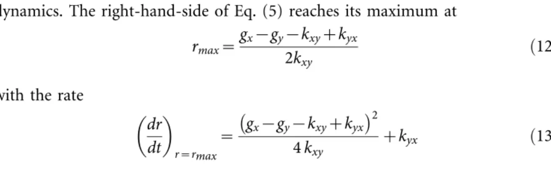
Figure 4. Three-phenotypic breast cancer cell population dynamics with both growth and transition from model simulation. A. Illustration of cell growth and transition for breast cancer cell line with three distinct cell phenotypes: luminal cell, basal cell and mammary stem cell.B1-B6. After FACS sorting, each isolated subpopulation of cell line SUM159, stem-like, basal and luminal cells, re-equilibrate to the stable cell-state ratior. Upper panels are the dynamics for cell numbers of three subpopulations; Lower panels are the dynamics for the cell ratios of three subpopulations.C1-C6. After FACS sorting, each isolated subpopulation of cell line SUM149, stem-like, basal and luminal cells, re-equilibrate to the stable cell-state ratior_{. Upper panels are the} dynamics for cell numbers of three subpopulations; Lower panels are the dynamics for the cell ratios of three subpopulations.

the transition rates, we have0_:05z0_:3v0_:69_,0_:01z0_:02=0_:91_,0_:03=0_:95_,

showing that the three subpopulations can all survive on their own as well. The dynamics for re-equilibrium of SUM159 cell line are shown inFig. 4B1-B6. We can clearly see that after cell sorting each cell sub-population quickly re-equilibrated to the stable steady-state ratior*5NX:NY:NZ<1.9:97.3:0.62 within 12 days. However, since SUM149 cell line generally has much slower transition rate, the population slowly re-equilibrated to the stable steady-state ratio until the end of the 140 days time-course, as shown inFig. 4C1-C6. Our computational results for both cell lines qualitatively agree with the experimental data and the Markov model simulation results presented in Gupta et al[18], which showed that SUM159 cells quickly returned to the equilibrium while SUM149 cells were far from reaching the equilibrium at day 6. Moreover, the ODE model revealed more information about cancer population dynamics. First, the ODE model computes the results for the cell population in real number, which is the gold standard for cancer drug evaluation. Second, we decided whether each cancer subpopulation can survive independently or as the derived one from other subpopulations. This finding has important implications during drug design, as it can inform which population is the more appropriated to target.

Discussion and Conclusion

Influence of the growth term in the cell population dynamics

We discuss the consequences of introducing the growth rate term for the steady state transition ratior~kyx=kxyin our two-phenotype model. Hereris the ratio

of cell numbers in the phenotype space, where each phenotype is determined by a state x of the cell’s molecular network. The dynamics of state x are captured by the transition rateskxy,kyx as well as the growth ratesgx,gy, which vary from state

to state. It offers both a rationale and a framework to understand the genotype-to-phenotype mapping problem in complex organisms [1,21–26]. If the growth rate is not included in Eq. (1) the steady state is simply given by the ratior~kyx=kxy.

The re-equilibrium is guaranteed in any situation, independent from the initial population ratio and from the transition rates. When the growth rate is

considered, there is no unconditional re-equilibrium for any transition rate. The growth ratesgx,gy and transition rateskyx,kxyhave to satisfy the condition defined

Table 1.The estimated values of growth rates and transition rates for breast cancer cell lines SUM159 and SUM149 to reach stable cell fraction ratior_after FACS sorting.

g_L g_S g_B KLS KLB KBL KBS KSL KSB

SUM159 0.73 0.69 0.85 0.04 0.42 0 0.012 0.14 0.33

SUM149 0.95 0.69 0.91 0.03 0 0.02 0.01 0.30 0.05

gL,gB,gSare growth rates of the subpopulation Luminal, Basal and cancer stem cells.Kij,ði~L,B,S;,j~L,B,SÞare transition rates between two breast cancer

cell subpopulations.

in Eq. (6). Also, to maintain two distinct cell subpopulations, it needs to satisfy the condition given by Eq. (4), i.e. transition rateskyx,kxyhave to be much smaller

than the growth rates gx,gy; otherwise, we will be in the presence of a cell

population with two indistinguishable subpopulations that can quickly transit between each other. In our ODE model for the breast cancer cell population dynamics, transition rates are indeed much smaller than the growth rate to guarantee independent existence of each cell population.

Selection vs. instruction dualism

By uniting the dynamics of reversible transitions between distinct cell phenotypes with their growth rates, we can capture the contributions for the evolution of the cell population from both Darwinian selection and Lamarckian induction. This has fundamental implications because evolutionary dynamics is commonly used to explain the changes that happen at tissue level during tumor progression [27– 33]. Since an attractor state confers a discrete, stable phenotype that can be inherited across cell divisions to future generations, we enter the new realm of non-genetic (mutation-less) Darwinian evolution. The fact that a cell phenotype (attractor) transition can be triggered by environmental perturbation also permits the consideration of Lamarckian evolution in cell populations during tumor progression, for which there are increasing evidences [19,20,34–40]. The general formalism combining state transitions and differential growth also reconciles the old debate between the selective (‘‘stochastic’’ or ‘‘permissive’’) vs. the instructive modes of cell fate determination during development [41–44]. Moreover, directed cell-to-cell interactions between cells in distinct states x mediated by the

expression of communication signals (cytokines), which are a function ofx, and affect proliferation and phenotype switching, can also be readily considered to incorporate non-cell autonomous effects in population dynamics [45].

The study of tissue change at the granularity of cell population dynamics also has direct impact on our understanding of the elementary principles of evolution. The macroscopic change of a population’s property X in a particular environment S in one direction can in principle be achieved by two mechanisms. Mechanism (i) is selection - in the presence of S, cells that ‘‘happen’’ to be stateyhave a higher growth rate (gywgx). There is no actual change of gene expression state in any cell

as this is a population level change. A core element of this process is randomness because the direction of change comes from the environment S. Mechanism (ii) is instruction: S induces a gene expression pattern change ðx?yÞin individual cells that confers a new phenotype. This is an individual cell level event, a change of the molecular network state of a cell. In evolution this dualism obviously maps into that of Darwinism vs. Lamarckism (in the case when the S-induced property endures and confers advantages in coping with S). Here we deal with a scheme of change and not its material cause [32]. Eq. (6) shows that fundamentally, in terms of schemes, Lamarckism and Darwinism are just the two sides of the very same dynamical process: (1) forgx{gy?kxy{kyx, (i.e. the difference of growth rates is

dominates in the dynamics of cell population ratio; (2) for the opposite case, when gx{gy=kxy{kyx, Lamarckian mechanism determines the cell population

ratio. Depending on the ‘‘half live’’ of the new induced state (relative stability) we would have inheritance of an acquired trait for at least several generations. In general the Darwinian scheme is invoked by default to explain cell differentiation, developmental processes and cancer origination. We propose that the alternative Lamarckian scheme also needs to be taken into account in the sense that either scheme has to be verified or falsified experimentally.

Conclusion

In this paper we provide a mathematical framework of population dynamics that considers both distinctive growth rates and intercellular transitions between cancer cell populations. Our mathematical framework showed that both growth and transition influence the ratio of cancer cell subpopulations, and transition’s role is even stronger. We derived the condition that different cancer cell types can maintain distinctive subpopulations and we also explain why there always exists a stable fixed ratio after the cell sorting based on certain surface markers. While Lamarckism has little role (if any at all) to play in organism evolution, our model is the first attempt to demonstrate that in principle Lamarckism and Darwinism (as an evolved adaptive response of a cell population) are two different sides of the same coin, two extremes of the same spectrum of behavioral schemes. This not only applies to the study of cancer cell dynamics, but also helps our understanding of the emergence of drug resistance in anti-cancer therapy.

Acknowledgments

We thank the helpful discussions with Aymeric Fouquier d’He´roue¨l, Ping Ao, Alex Skupin and Xiaojie Qiu.

Author Contributions

Conceived and designed the experiments: JZ HQ SH. Performed the experiments: JZ AOP. Analyzed the data: JZ. Contributed reagents/materials/analysis tools: HQ AOP. Wrote the paper: JZ HQ SH.

References

1. Huang S (2011) The molecular and mathematical basis of Waddington’s epigenetic landscape: A framework for post-Darwinian biology? BioEssays: 1–15. doi:10.1002/bies.201100031.

2. Delbru¨ ck M(1949) in Unite´s biologiques doue´es de continuite´ ge´ne´tique Colloques Internationaux du Centre National de la Recherche Scientifique.

3. Kauffman S(1969) Homeostasis and differentiation in random genetic control networks. Nature 224: 177–178.

5. Bornholdt S(2008) Boolean network models of cellular regulation: prospects and limitations. Journal of the Royal Society, Interface/the Royal Society 5 Suppl 1: S85–S94.

6. Zhou JX, Huang S (2011) Understanding gene circuits at cell-fate branch points for rational cell reprogramming. Trends in genetics: TIG 27: 55–62. doi:10.1016/j.tig.2010.11.002.

7. Zhou JX, Aliyu MDS, Aurell E, Huang S(2012) Quasi-potential landscape in complex multi-stable systems. Journal of the Royal Society, Interface/the Royal Society 9: 3539–3553. doi:10.1098/ rsif.2012.0434.

8. Zhou JX, Brusch L, Huang S(2011) Predicting Pancreas Cell Fate Decisions and Reprogramming with a Hierarchical Multi-Attractor Model. PLoS ONE 6: e14752. doi:10.1371/journal.pone.0014752.

9. Nowak M(2006) Evolutionary Dynamics: Exploring the Equations of Life. Belknap Press. p.

10. Zheng Q (Natioanal center for toxicological research)(1999) Progress of a half century in the study of the Luria¡Delbr uck distribution. Mathematical Biosciences 162: 1–32.

11. Saunders NJ, Moxon ER, Gravenor MB(2003) Mutation rates: Estimating phase variation rates when fitness differences are present and their impact on population structure. Microbiology 149: 485–495.

12. Attolini CSO, Michor F (2009) Evolutionary theory of cancer. Annals of the New York Academy of Sciences 1168: 23–51.

13. Huang S(2009) Non-genetic heterogeneity of cells in development: more than just noise. Development (Cambridge, England) 136: 3853–3862.

14. Altschuler SJ, Wu LF(2010) Cellular Heterogeneity: Do Differences Make a Difference? Cell 141: 559– 563.

15. Balaban NQ, Merrin J, Chait R, Kowalik L, Leibler S(2004) Bacterial persistence as a phenotypic switch. Science (New York, NY) 305: 1622–1625.

16. Fu Y, Zhu M, Xing J (2010) Resonant activation: a strategy against bacterial persistence. Physical biology 7: 16013.

17. Singh DK, Ku C-J, Wichaidit C, Steininger RJ, Wu LF, et al. (2010) Patterns of basal signaling heterogeneity can distinguish cellular populations with different drug sensitivities. Molecular systems biology 6: 369.

18. Huang S (2013) Genetic and non-genetic instability in tumor progression: Link between the fitness landscape and the epigenetic landscape of cancer cells. Cancer and Metastasis Reviews 32: 423–448.

19. Pisco AO, Brock A, Zhou J, Moor A, Mojtahedi M, et al.(2013) Non-Darwinian dynamics in therapy-induced cancer drug resistance. Nature communications 4: 2467. doi:10.1038/ncomms3467.

20. Gupta PB, Fillmore CM, Jiang G, Shapira SD, Tao K, et al.(2011) Stochastic State Transitions Give Rise to Phenotypic Equilibrium in Populations of Cancer Cells. Cell 146: 633–644. doi:10.1016/ j.cell.2011.07.026.

21. Atallah J, Larsen E(2009) Chapter 3 Genotype-Phenotype Mapping. Developmental Biology Confronts the Toolkit Paradox. International Review of Cell and Molecular Biology 278: 119–148.

22. Kell DB(2002) Genotype-phenotype mapping: genes as computer programs. Trends in genetics: TIG 18: 555–559. doi:10.1016/S0168-9525(02)02765-8.

23. Mehmood T, Warringer J, Snipen L, Sæbø S (2012) Improving stability and understandability of genotype-phenotype mapping in Saccharomyces using regularized variable selection in L-PLS regression. BMC Bioinformatics 13: 327.

24. Nuzhdin SV, Friesen ML, McIntyre LM(2012) Genotype-phenotype mapping in a post-GWAS world. Trends in Genetics 28: 421–426.

25. Pigliucci M(2010) Genotype-phenotype mapping and the end of the ‘‘genes as blueprint’’ metaphor. Philosophical transactions of the Royal Society of London Series B, Biological sciences 365: 557–566. doi:10.1098/rstb.2009.0241.

26. Wu C, Walsh AS, Rosenfeld R(2011) Genotype phenotype mapping in RNA viruses - disjunctive normal form learning. Pacific Symposium on Biocomputing Pacific Symposium on Biocomputing: 62–73.

28. Dowty JG, Byrnes GB, Gertig DM(2013) The time-evolution of DCIS size distributions with applications to breast cancer growth and progression. Mathematical medicine and biology: a journal of the IMA: 1– 12. doi:10.1093/imammb/dqt014.

29. Newburger DE, Kashef-Haghighi D, Weng Z, Salari R, Sweeney RT, et al.(2013) Genome evolution during progression to breast cancer. Genome Research 23: 1097–1108.

30. Yachida S, Iacobuzio-Donahue C(2013) Evolution and dynamics of pancreatic cancer progression. Oncogene 32: 5253–5260.

31. Durrett R, Moseley S(2010) Evolution of resistance and progression to disease during clonal expansion of cancer. Theoretical Population Biology 77: 42–48.

32. Klein CA(2004) Gene expression sigantures, cancer cell evolution and metastatic progression. Cell cycle (Georgetown, Tex) 3: 29–31.

33. Armengol G, Capella` G, Farre´ L, Peinado MA, Miro´ R, et al.(2001) Genetic evolution in the metastatic progression of human pancreatic cancer studied by CGH. Laboratory investigation; a journal of technical methods and pathology 81: 1703–1707.

34. Dallas N, Xia L, Fan F, Gray MJ, Gaur P, et al.(2009) Chemoresistant colorectal cancer cells, the cancer stem cell phenotype, and increased sensitivity to insulin-like growth factor-I receptor inhibition. Cancer research 69: 1951–1957. doi:10.1158/0008-5472.CAN-08-2023.

35. Lee G-Y, Shim J-S, Cho B, Jung J-Y, Lee D-S, et al.(2011) Stochastic acquisition of a stem cell-like state and drug tolerance in leukemia cells stressed by radiation. International journal of hematology 93: 27–35. doi:10.1007/s12185-010-0734-2.

36. Yang AD, Fan F, Camp ER, Van Buren G, Liu W, et al.(2006) Chronic oxaliplatin resistance induces epithelial-to-mesenchymal transition in colorectal cancer cell lines. Clinical cancer research: an official journal of the American Association for Cancer Research 12: 4147–4153. doi:10.1158/1078-0432.CCR-06-0038.

37. Chaffer CL, Weinberg R(2011) A perspective on cancer cell metastasis. Science (New York, NY) 331: 1559–1564. doi:10.1126/science.1203543.

38. Lagadec C, Vlashi E, Della Donna L, Dekmezian C, Pajonk F (2012) Radiation-induced reprogramming of breast cancer cells. Stem Cells 30: 833–844.

39. Wen K, Fu Z, Wu X, Feng J, Chen W, et al.(2013) Oct-4 is required for an antiapoptotic behavior of chemoresistant colorectal cancer cells enriched for cancer stem cells: Effects associated with STAT3/ Survivin. Cancer Letters 333: 56–65.

40. Zhang R, Zhang Z, Zhang C, Zhang L, Robin A, et al. (2004) Stroke transiently increases subventricular zone cell division from asymmetric to symmetric and increases neuronal differentiation in the adult rat. The Journal of neuroscience: the official journal of the Society for Neuroscience 24: 5810– 5815.

41. Coffman RL (1999) Instruction, Selection, or Tampering with the Odds? Science 284: 1283–1285. doi:10.1126/science.284.5418.1283.

42. Enver T, Heyworth CM, Dexter TM(1998) Do stem cells play dice? Blood 92: 348–51; discussion 352.

43. Enver T, Jacobsen SEW(2009) Developmental biology: Instructions writ in blood. Nature 461: 183– 184.

44. Metcalf D(1998) Cell-cell signalling in the regulation of blood cell formation and function. Immunology and cell biology 76: 441–447. doi:10.1046/j.1440-1711.1998.00761.x.