The noise and the KISS in the cancer stem cells niche

The noise and the KISS in the cancer stem cells niche

Renato Vieira dos Santos

a,n

, Linaena Méricy da Silva

b,c

a_{Departamento de Física, Instituto de Ciências Exatas, Universidade Federal de Minas Gerais, CP 702, CEP 31270-901 Belo Horizonte, Minas Gerais, Brasil} b_{Centro Universitário Metodista Izabela Hendrix, Núleo de Biociências, Rua da Bahia 2020, CEP 30160-012, Belo Horizonte, Minas Gerais, Brasil} c_{Laboratório de Patologia Comparada, Instituto de Ciências Biológicas, Universidade Federal de Minas Gerais, CP 702, CEP 31270}

–901 Belo Horizonte, Minas Gerais, Brasil

H I G H L I G H T S

Possible explanation for wide variability observed in cancer stem cells frequency.

Plasticity is necessary for maintenance of cancer stem cell populations.

Cell population may exhibit a noise-induced transition.

a r t i c l e i n f o

Article history:

Received 15 December 2012 Received in revised form 8 May 2013

Accepted 21 June 2013 Available online 1 July 2013

Keywords: Cancer stem cells Stochastic modeling Minimal patch size Plasticity Diffusion

a b s t r a c t

There is a persistent controversy regarding the frequency of cancer stem cells (CSCs) in solid tumors. Initial studies indicated that these cells had a frequency ranging from 0.0001% to 0.1% of total cells. Recent studies have shown that this does not seem to be always the case. Some of these studies have indicated a frequency of 40%. Through a simple population dynamics model, we studied the effects of stochastic noise and cellular plasticity in the minimal path size of a cancer stem cells population, similar to what is done in what is sometimes called the Kierstead–Skellam–Slobodkin (KISS) Size analysis. We show that the possibility of large variations in the results obtained in the experiments may be a consequence of the different conditions under which the different experiments are submitted, specifically regarding the effective cell niche size where stem cells are transplanted. We also show the possibility of a noise induced transition where the stationary probability distribution of the CSC population can present bimodality.

&2013 Elsevier Ltd. All rights reserved.

1. Introduction

In recent years there has been increasing evidence for the

Cancer Stem Cell(CSC) hypothesis (Reya et al., 2001; Clarke and Fuller, 2006;Vermeulen et al., 2008;Dalerba et al., 2007), accord-ing to which tumor formation is a result of genetic and epigenetic changes in a subset of stem-like cells, also known astumor-forming

ortumor-initiatingcells (Bomken et al., 2010). Cancer stem cells werefirst identified in various leukemias and, more recently, in several solid tumors such as brain, breast, cervix and prostate tumors (Dalerba et al., 2007).

It has been suggested that these are the cells responsible for initiating and maintaining tumor growth. In this paper, we study a model for tumor growth that assumes the existence ofcancer stem cells(CSCs), ortumor initiating cells.

The conceptual starting point relevant to CSC theory is con-structed from the known heterogeneity of tumors. We now know

that cells in a tumor are not all identical copies of each other, but that they display a striking array of characteristics (Denison, 2012;

Tian et al., 2011; Shackleton et al., 2009; Marusyk and Polyak, 2010;Marusyk et al., 2012). CSC theory recognizes this fact and develops its consequences. And one of the most immediate implications for clinical practice is that conventional treatments can generally attack the wrong cell type. The appeal of the CSC idea can be described by the following analogy: just as killing the queen bee leads to the demise of the hive, destroying cancer stem cells, should, in theory, stop a tumor from renewing itself. Unfortunately, things are never that simple. In the hive, workers react quickly to the death of the queen by replacing her with a new one. And there is some evidence (Welte et al., 2010; Rapp et al., 2008) to suggest that could also happen in tumors due to a phenomenon known ascell plasticity, which allows normal tumor cells to turn into cancer stem cells, should the situation call for it. One goal of this study is to evaluate the possible effects of this plasticity. Analogies with superorganisms such as bee colonies are taken much more seriously inGrunewald et al. (2011).

Stem cells in general (the same applies to CSCs) tend to be found on specific areas of a tissue where one particular Contents lists available atSciVerse ScienceDirect

journal homepage:www.elsevier.com/locate/yjtbi

Journal of Theoretical Biology

0022-5193/$ - see front matter&2013 Elsevier Ltd. All rights reserved. http://dx.doi.org/10.1016/j.jtbi.2013.06.025

n

Corresponding author. Tel.:+51 3133737186.

microenvironment, calledniche(Lander et al., 2012), promotes the maintenance of its vital functions. This niche has specialized in providing factors that prevent differentiation and thus maintain the stemness of CSCs and, ultimately, the tumor's survival. Stem cells and niche cells interact with each other via adhesion molecules and paracrine factors. This complex network of interac-tions exchanges molecular signals and maintains the unique char-acteristics of stem cells, namely, pluripotency and self-renewal.

Given the extreme complexity of the cellular microenvironment in general and of the niche in particular (Iwasaki and Suda, 2009;

Lander et al., 2012), we will formulate an effective stochastic theory for the population dynamics of CSCs. We are especially interested in investigating a controversy related to the frequency with which CSCs appear in various tumors (Ishizawa et al., 2010;Stewart et al., 2011;Vargaftig et al., 2011;Sarry et al., 2011;Zhong et al., 2010;

Baker, 2008a,b; Johnston et al., 2010). In the initial version of CSC theory, it was believed that these cells were a tiny fraction of the total, ranging from 0.0001% to 0.1% (Schatton et al., 2008;Quintana et al., 2008). However, more recent studies have shown a strong dependence on the number of stem cells present in a tumor with the xenograft experimental model used. In explicit contrast to what was previously thought, inQuintana et al. (2008)a CSC proportion of approximately 25% was observed. Other studies have confirmed this observation (Kelly et al., 2007;Williams et al., 2007;Schatton et al., 2008), with the proportion potentially reaching 41% (Boiko et al., 2010). InGupta et al. (2009)the authors provide evidence that this discrepancy may be caused by the possibility of phenotypic switching between different tumor cells. By phenotypic switching we mean that a more differentiated cancer cell can, under appro-priate conditions, de-differentiate into a cancer stem cell. This is the cellular plasticity mentioned above.

In Zapperi and La Porta (2012), it is suggested that inconsis-tencies in the numbers of cancer stem cells reported in the literature can also be explained as a consequence of the different de_finitions used by different researchers. Different assays will give different numbers of cells, which can be orders of magnitude away from each other.

In this paper we are also interested in knowing what are the possible effects of cells diffusion in space. For this, we constructed bifurcation diagrams that show how the population size of CSCs varies when the size of the niche cells changes. We consider the effects that the plasticity phenomenon as well as spatio-temporal noise can have in these diagrams. Finally we studied the effects of the spatial distribution of cells in stationary probability distributions.

The paper is organized as follows: inSection 2 we explain the basic assumptions of our model of CSC population dynamics. In

Section 3we describe the set of reactions we use in the models. The effects of inclusion of spatial structure in the analysis are considered inSection 4.Section 5closes the paper with conclusions.

2. Assumptions

Mathematical modeling has made significant contributions to our understanding of the biology of cancer since the pioneering work ofNordling (1953)andArmitage and Doll (1954), in which the authors proposed that multiple mutations may explain the data on the incidence of cancer and its correlation with age (Chen et al., 2005; Horov et al., 2009). For historical reviews on the subject, seeMcElwain and Araujo (2004)andByrne et al. (2006). In the model used in this paper, cancer stem cells can perform three types of divisions, according toMorrison and Kimble (2006):

Symmetric self-renewal: Cell division in which both daughter cells have the characteristics of the stem cell mother, resulting in an expanding population of stem cells.

Symmetric differentiation: A stem cell divides into two prog-enitor cells.

Asymmetric self-renewal: A cancer stem cell (denoted byC) is generated and a progenitor cell (mature cancer cell, denoted by

P) is also produced.

We developed a simple mathematical model for the stochastic dynamics of CSCs in which the three division types possess intrinsic replication rates, which are assumed to be time-independent. Therefore, besides these division types, we assume that there is also the possibility of a transformation in which a progenitor cell can acquire characteristics of stem cells where, for all practical purposes, we may regard it as having become a de-differentiated stem cell. In mixed lineage leukemia cells, it was recently shown that committed myeloid progenitor cells acquire properties of leukemia stem cells without changing their overall identity (Leder et al., 2010). These cells do not become stem cells, but rather develop stem cell like behavior by re-activating a subset of genes highly expressed in normal hematopoietic stem cells (Rapp et al., 2008). The biological mechanisms underlying this transformation are described inGupta et al. (2009), for example. As mentioned previously, we refer to this process ascell plasticity.

3. Model

This section describes the basic model investigated in this paper. It is based on the cell division mechanism and the plasticity property. We will use the language of stochastic differential equations (Karlin and Taylor, 2000;Schuss, 2010;Oksendal, 2003). The model is a natural extension of the one proposed inTurner et al. (2009). This extension refers to the inclusion of competition between cells because of the scarcity of resources when popula-tions become large enough. This new possibility in relation to the model proposed inTurner et al. (2009)makes the model nonlinear and prevents that the populations tend to infinity. The model is described in the next subsection.

3.1. The basic model

We assume that the population dynamics of cancer stem cells and progenitor cells are governed by the following reactions:

C ⇌k1 k′2=Ω2

CþC

P ⇌ k3

k′4=Ω4

P_þP

C, k5

CþP

C, k6

PþP

P, k7 ∅

P, k8

C ð1Þ

The_first and second reactions, in the forward sense, model cell proliferation, which occurs at a rate k1 and k3, respectively.

Constantsk′2 and k′4 are associated to the reverse process and describe the intensity of competition between the CSC and progenitor cells, respectively, and prevents their unlimited expo-nential growth;Ω2 and Ω4 are constants related to the model's

carrying capacity. The third reaction involvingk5originates from

the asymmetric transformation of CSCs in CSC daughter and progenitor cell types. The reaction involving the ratek6is related

All rates have dimension (time) 1_{. The speci}

fic unit of time (months, quarters, years, etc.) will depend on the type and aggressiveness of the tumor.

Using the law of mass action, we can write

dC

dt¼k1C k2C

2 _k 6Cþk8P

dP

dt¼k3P k4P

2

þ ðk5þ2k6ÞC ðk7þk8ÞP 8

> > <

> > :

ð2Þ

with k2≡k′2=Ω2, k4≡k′4=Ω4. Setting ΩC≡k1=k2, ΩP≡k3=k4, k9≡k5þ

2k6 and k10≡k7þk8 and making the substitutions C¼ΩCx,

P¼ΩC ffiffiffiffiffiffiffiffiffiffiffiffi

k9=k2 p

y and t¼τ=k6, Eq. (2) can be written as (see Appendix A)

dx

dτ¼Axð1 xÞ xþBy≡fðx;yÞ

dy

dτ¼Eyð1 FyÞ þBx Gy≡gðx;yÞ 8

> > <

> > :

ð3_Þ

with

A≡k1

k6

B≡ ffiffiffiffiffiffiffiffiffiffi

k2k9 p

k6

E≡k3

k6

F≡ΩC ΩP

ffiffiffiffiffi

k9

k2 s

G≡k10

k6 8

> > > > > > > > > > > > > > > > > > <

> > > > > > > > > > > > > > > > > > :

ð4Þ

As∂_f=∂_y¼∂_g=∂_{x¼B, Eq.(3)represents a gradient system (Perko,} 2000) with potentialVðx;yÞgiven by

Vðx;yÞ ¼1₆ð3 3Aþ2AxÞx2 _Bxyþ1

6ð3G 3Eþ2EFyÞy

2_{: ð5Þ}

As a consequence (Hirsch et al., 2004):

1. The eigenvalues of the linearization of Eq. (3) evaluated at equilibrium point are real.

2. If ðx0;y0Þ is an isolated minimum of V then ðx0;y0Þ is an

asymptotically stable solution of(3).

3. If_ðx_ðτÞ;y_ðτÞÞis a solution of(3)that is not an equilibrium point thenVðxðτÞ;yðτÞÞis a strictly decreasing function and is perpen-dicular to the level curves ofVðx;yÞ.

4. There are no periodic solutions of(3).

Fig. 1shows the potential functionVðx;yÞ. Suf_ficiently smallF

(ΩP≫ΩC) implies large differences in equilibrium populations ofC

and P. For parameters A¼B¼G¼1, E¼3 and F¼0:01,

ðx0;y0Þ ¼ ð8:4;70:6Þ. If we setF¼0:0001, keeping the other

para-metersfixed, we getðx0;y0Þ ¼ ð82;6710Þ.

3.2. Adiabatic elimination

The proposed model in(1)is in fact a general model of stem cells and does not even carry any speci_fic characteristic of cancer stem cells. All properties considered, such as plasticity and changes in the microenvironment conditions (to be included later), are also found in stem cell systems of normal tissue. The features associated with cancer stem cells are related to the large carrying capacity of progenitor cells when compared with the carrying capacity of cancer stem cells. This fact is represented numerically by the choice of model parameters made below, which results in this discrepancy.

We can write(2)in the form (seeAppendix A)

x′¼A′xð1 xÞ xþB′y y′¼E′yð1 yÞ þF′x G′y

(

ð6Þ

withx′≡dx=dt′,y′≡dy=dt′,t′≡t=k6and

A′≡k1

k6

B′≡k2k3k8

k1k4k6

E′≡k3

k6

F′≡k1k4k9

k2k3k6

G′≡k10

k6 8

> > > > > > > > > > > > > > > > > <

> > > > > > > > > > > > > > > > > :

ð7_Þ

Fig. 2shows the numerical solutions of Eqs.(6)(the rescaled equation) and (2) for the following parameter values: k1¼

1 k5 k6, k2¼410 13, k3¼1, k4¼10 13, k5¼0:1, k6¼0:1,

k7¼0.1 and k8¼0:00001.1 We make the usual assumption

(k1þk5þk6Þb¼1 (Tomasetti and Levy, 2010), where β≡ 1 is a

general parameter with dimension time( 1)_{required for}

dimen-sional consistency in the following analysis. The values fork5and k6 are consistent with those estimated in Tomasetti and Levy (2010). For these parameter values, ΩC≡k1=k2¼21012 and ΩP≡k3=k4¼11013 (see Appendix A). These are rescaling

para-meters forxandyvariables, respectively. Stationary values forP(t) and C(t) are P₁¼9:61012 _{cells and C}

1¼1:81012 cells,

respectively. By adjusting thek2andk4parameters we can easily

obtain more suitable values for the CSC and progenitor cell equilibrium populations, according to possible new experimental results.

By using standard adiabatic elimination methods, one can write Eq.(6)as

x′¼A′ xð1 xÞ _Ax

′ þ

B′

A′y

ϵy′¼yð1 yÞ þϵF′x ϵG′y

8

> <

> :

ð8Þ

whereϵ≡1=E_′. If we considerϵ≪1 (this is equivalent to considering the progenitor cell division rate sufficiently large) we can perform

Fig. 1.PotentialVðx;yÞfrom Eq.(5)for parametersA¼B¼G¼1,E¼3 andF¼0.01.

1_{These values correspond toA}

′¼8,B′¼510 4_,E

adiabatic approximation (Berglund and Gentz, 2006; Gardiner, 2009) in(8)and, settingy_′¼0, we obtain the following equation2

forx:

x′¼χ μxþαxð1 xÞ ð9Þ

where χ≡_{B′ð1 ϵG′Þ ¼k8k2ðk3 k10Þ=k1k4k6, μ}≡_{1 ϵB′F′¼1 k8k9=}

k3k6 and α≡A′¼k1=k6. Note that χ can be positive or negative

depending on the magnitudes ofk3andk10.

If we considerϵto be small enough with respect toG′,B′andF′, we further simplify and writeχ¼B′andμ¼1. We can observe that the plasticity phenomenon (associated withk8) is crucial for the

existence of the constant termχ. For this reason, from now on we will consider the parameter χ as representing the plasticity phenomenon in the reduced equation(9).

3.3. The deterministic equation

We will brie_fly review the deterministic analysis of the pro-blem. An analytic solution of Eq. (9) is possible. For the initial conditionxð0Þ ¼N0, we get

xðtÞ ¼₂1

α δ ffiffiffi κ

p

tan 1 2t

ffiffiffi κ

p

þarctan 2N0αffiffiffiþδ κ

p

ð10Þ

withδ≡_{α μ}andκ≡ _δ2 4αχ. The physically relevant stable _fixed point is

xn

¼α μþ

ffiffiffiffiffiffiffiffiffiffiffiffiffiffiffiffiffiffiffiffiffiffiffiffiffiffiffiffiffiffiffiffiffiffiffiffiffiffiffiffiffi α2 _2αμþμ2_þ4αχ p

2α : ð11Þ

The xscaled population size dynamics can be thought of as analogous to the particle moving dynamics in an effective poten-tialV0ðxÞ, seeking its minimum point, withV0ðxÞ≡ RζðxÞdxwith ζðxÞ ¼χþδx αx2 _{from (9). Thus, V}

0 is given by the cubic

polynomial,

V0ðxÞ ¼

x3_α

3

δx2

2 xχ:

We see from(11)that by increasing eitherχorδ, the minimumxn

ofV0moves to the right in the potential, thus favoring the tumor

stem cell population. Such behavior is, of course, expected, since an increase ofχmeans an increase of the frequency in which the induced plasticity mechanism occurs, and an increase ofδis an increase of the symmetric stem cell renewal rate, both of which increase the population.

4. Possible consequences of a spatial structure

Traditionally, anti-tumor treatments have targeted the cells directly, removing them with surgery or killing them with radia-tion. Since these are local treatment methods, they often are not effective in meeting their objectives. The tumors may recur because not all cells were killed or because some cells escaped the primary tumor region where the treatments worked. Since cells compete and/or cooperate with nontumor cells and between themselves, these interactions may be better conceptualized as an evolving ecosystem (Pienta et al., 2008;Kareva, 2011).

One of the possible consequences of this way of seeing the disease is that the destruction of the tumor microenvironment can be much more effective than just extracting or killing the cells that live in it. A prime example of this situation comes from paleontol-ogy: studies analyzing the conditions that preceded mass extinc-tions suggest that they occurred more frequently and were more destructive when pulses of disturbances that cause extensive mortality were accompanied by perturbative pressures such as climate change. This sequence weakened and destabilized popula-tions for several generapopula-tions (Arens and West, 2008).

Motivated by these considerations, it seems promising to consider mathematical techniques originating in mathematical ecology, a well-developed branch of applied mathematics (Cantrell and Cosner, 2003;Petrovskii and Li, 2005). We are now interested in the possible effects from the incorporation of diffu-sion in the model. For this, letuðx;tÞbe a population of CSCs at position x at time t that lives in a one-dimensional domain of lengthL. By adding a diffusion term in Eq.(9), we get

∂u

∂t′¼D ∂2_u

∂t′2þχ μuþαuð1 uÞ≡D

∂2_u

∂t′2þfðuÞ ð12Þ

whereDis the cell diffusion coefficient andfðuÞ ¼χ μuþαuð1 uÞ. This is the deterministic partial differential equation that we will consider_first. Later we will consider a stochastic version. This is a reaction diffusion equation that is typical in the population dynamics of species that interact and disperse.

Eq.(12)withχ¼0 is the famousFisher (1937)equation. In this equation we analyze the effect of plasticity represented by the parameterχon the patch size to sustain a population, similar to what is sometimes called the Kierstead–Slobodkin–Skellam (KISS) size (Skellam, 1951; Kierstead and Slobodkin, 1953). The main motivation for performing this type of analysis is related to the experimental results obtained in Quintana et al. (2008), where xenografts in immunosuppressed mice sustained surprisingly high populations of cancer stem cells. The idea here, therefore, is to identify some phenomenon related to the size of the CSC niche that may justify this result. The question is: What is the effect of transplanting a cancer stem cell population to an environment where, in theory, they will have more space to live and proliferate? To formulate the problem mathematically, we can imagine that there is a_finite domain available for the cells to develop (their niche). Beyond a certain boundary (i.e. outside the niche), there

0

1

2

0

0.6

1.2

0

25

50

Fig. 2.Top: numerical solution for rescaled Eq.(6). x(t) and y(t) represent the

rescaled population of cancer stem cells and progenitor cells, respectively. Bottom: numerical solution for Eq.(2).C(t) andP(t) represent the population of cancer stem cells and progenitor cells, respectively.P1andC1represent the limits ofC(t) and P(t) whent-1, respectively. Parameters values:k1¼1 k5 k6,k2¼410 13, k3¼1,k4¼10 13,k5¼0:1,k6¼0:1,k7¼0.1 andk8¼0:00001.P1¼9:61012and C1¼1:81012.C1=P1¼0:1875.

are restrictions (e.g., absence of signaling to support the cancer stem cell phenotype, normoxic conditions incompatible with the state of CSCs, adverse pH conditions, etc.) which make the survival of cancer stem cells unsustainable. Outside the niche, these cells have a tendency to differentiate into progenitor cells. Thinking of the niche as a linear domain of length L, our problem can be mathematically formulated as a boundary value problem with Dirichlet conditions given by(12)and

uð0;t′Þ ¼uðL;t′Þ ¼0:

FollowingMéndez et al. (2008), the population density at the steady state is given by uðx;1Þ≈_{um sinðπx=LÞ, where um is the}

maximum population density at steady state for a given patch sizeL. In Méndez et al. (2008), for a function f_ðu_Þ in the form

fðuÞ ¼a1uþa2u2þa3u3, an approximation toumis found as the

real solution to the equationΦðum;LÞ ¼0 with

Φðum;LÞ≡um

3a3

4 u

2 mþ

8a2

3πumþa1 D π

L

2

: ð13Þ

Allowing the possibility of plasticity (represented by χ), we insert a term a0 in the f(u) function so that fðuÞ ¼a0þ

a1uþa2u2þa3u3. By performing the calculations as in Méndez et al. (2008), we obtain the new function

Φχðum;LÞ ¼

4a0 π þum

3a3

4 u

2 mþ

8a2

3π umþa1 D π

L

2

: ð14Þ

By solving equationΦχðum;LÞ ¼0, we get three solutions that,

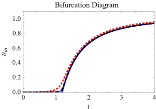
when placed on the same figure, make up what we call a bifurcation diagram (ifχ¼0).3 _Fora

0¼χ,a1¼α μ,a2¼ αand

a3¼0, we consider the case of Eq.(12).

Fig. 3shows the bifurcation diagram forχ¼0 (blue curve) and the curvesumðLÞforχ¼0:1 (dotted red curve) andχ¼0:01 (black

dashed curve). We_find that the inclusion of plasticity allows small cancer stem cell populations to survive even in very small niches. Above a certain approximate critical minimum value for patch size (KISS size Lc¼πpffiffiffiffiffiffiffiffiffiffiffiD=a1), the population undergoes an abrupt

increase in its size. If a small cell niche is abruptly increased to a value significantly greater than Lc, the CSC population will be

absurdly high. This may have been the case for the xenograft cancer stem cells in immunosuppressed mice reported inQuintana et al. (2008). This may also be an answer to the question raised above.

4.1. Effect of noise on the bifurcation diagram

4.1.1. Noise in the cancer stem cell niche

Cells growing in a tissue are not alone: they are constantly communicating with one another by sending signals through tissue that are picked up and transmitted by other cells in the medium. When thousands of cells are together, there are hundreds of thousands of these signals present every minute, all competing to be heard. All this complexity induces stochastic_fluctuations in population dynamics that will hereafter be called noise.

A growing body of evidence indicates that noise is generally not detrimental to biological systems, but can be employed to gen-erate behavioral diversity (Samoilov et al., 2005; Fange and Elf, 2006). Mechanisms involving noise are important in the develop-ment of organisms (Arias and Hayward, 2006; El-Samad and Khammash, 2006), a fact supported by experiments showing that noise is down-regulated in embryonic stem cells (Zwaka, 2006) and thatfluctuations of the Nanog transcription factor predispose these cells towards differentiation (Chambers et al., 2007;Kalmar

et al., 2009). InHoffmann et al. (2008)it was suggested that the regulation of noise can be an effective strategy in stem cell differentiation. The results of the present paper suggest that high levels of noise can stimulate the development of cancer stem cells.

4.1.2. Modeling noise in a spatial environment

We will now reformulate the population dynamics in terms of a stochastic reaction–diffusion equation and reduce it to a determi-nistic equation that incorporates the systematic noise contribu-tions (Santos and Sancho, 2001). Let usfirst formulate the problem in a general way and then use our model as an example.

Consider the following stochastic partial differential equa-tion (SPDE) in the Stratonovich interpretaequa-tion, with both additive and multiplicative noises:

∂ϕ

∂t ¼D∇

2_{ϕþfðϕÞ þϵ}1=2_{gðϕÞηðx;tÞ þξðx;tÞ: ð15Þ}

In the above equation,ϵis an explicit measure of the noise strength given byηðx;tÞ,ϕðx;tÞis a_field (scalar or vector) that describes the state of the system (the number of CSCs in our context) at a spatial locationxat timet, and Dis the diffusion coefficient. The additive noiseξðx;tÞis Gaussian and white in both space and time, with zero mean and correlations given by

〈ξðx;tÞξðx′;t′Þ〉¼2γ2δðx x′Þδðt t′Þ:

The multiplicative noise ηðx;tÞ is Gaussian, with zero mean and correlation

〈ηðx;t_Þηðx′;t′Þ〉¼2c_ðjx x′jÞδðt t′Þ

withcðjx x′jÞas the spatial correlation function. A crucial feature of

(15)is that whileηðx;tÞhas zero mean, our new noise termgðϕÞηðx;tÞ

does not. Ifg_ðϕÞis constant, Eq.(15)has only additive noise. In our case however, noise is coupled to the system through functiong.

4.1.3. Effective deterministic model

As mentioned above, the new noise term has nonzero mean. We de_fine it as follows:

ϵ1=2〈g_ðϕÞηðx;t_Þ〉≡ΨðϕÞ: ð16_Þ

Adding and subtractingΨðϕÞin(15)lead to an equivalent equation, but with zero mean noise termR

∂ϕ

∂t ¼D∇

2_{ϕþfðϕÞ þΨðϕÞ þRðϕ;x;tÞ ð17Þ}

where

Rðϕ;x;tÞ ¼ϵ1=2gðϕÞηðx;tÞ ΨðϕÞ þξðx;tÞ: ð18Þ Rðϕ;x;tÞis related to the nonsystematic noise effect. This effect will

0 1 2 3 4

0.0 0.2 0.4 0.6 0.8 1.0

L

u

m

Bifurcation Diagram

Fig. 3.Bifurcation diagram obtained fromΦχðum;LÞ ¼0 withΦχðum;LÞgiven by

Eq.(14)withχ¼0:0 (blue, thick line),χ¼0:1 (red, dotted line),χ¼0:01 (black, dashed line),μ¼1,α¼8. (For interpretation of the references to color in thisfigure caption, the reader is referred to the web version of this paper.)

be neglected (Santos and Sancho, 2001), thus leading to an effective deterministic equation

∂ϕ

∂t ¼D∇

2_{ϕþfðϕÞ þΨðϕÞ ð19Þ}

with an effective reaction termfðϕÞ þΨðϕÞ.ΨðϕÞcan be calculated usingNovikov's (1965)theorem producing

ϵ1=2〈gðϕÞηðx;tÞ〉¼ϵcð0Þ〈g′ðϕÞgðϕÞ〉: ð20Þ

The deterministiceffectivemodel is written as

∂ϕ

∂t ¼D∇

2_ϕ

þf_ðϕÞ þϵc_ð0_Þg′ðϕÞg_ðϕÞ: ð21_Þ

4.1.4. Application to our model

Considering the inclusion of a Gaussian noise of intensitysin parameter α,4 _{(by the transformation α}

-αþsWðtÞ, W(t) is a

Wiener process Oksendal, 2003) we get a model corresponding to Eq. (15) with fðϕÞ ¼χþ ðα μÞϕ αϕ2 (a polynomial of degree two) and gðϕÞ ¼ϕð1 ϕÞ. Therefore, the effective deterministic model is given by

∂ϕ

∂t ¼D∇

2_{ϕþχþ ðα μþsÞϕ ðαþ3sÞϕ}2_þ2sϕ3 _ð22Þ

or

∂ϕ

∂t ¼D∇

2_ϕ

þχþMϕ Nϕ2þPϕ3 ð23_Þ

withM≡_{α μþs,N}≡_αþ3s,P≡_2sands≡_{ϵcð0Þ. Besides the}

renor-malization in parametersμ and α, the degree of the polynomial function to the right of (22) is lifted from two to three. The systematic contributions of the noise in the proliferation rate give rise to a cubic term in the effective reaction function. Conse-quently, the validity range of Eq.(23)is restricted to sufficiently small noise strengths or small densities. This does not affect our conclusions, since we are interested in the conditions for extinc-tions, i.e., situations where the density is indeed small. At higher densities, the model needs to be modified to include higher-order saturation effects.

It is interesting to observe the effect of s on the effective potential VeffðϕÞ associated with the model without diffusion,

obtained fromVeffðϕÞ ¼ R

½fðϕÞ þΨðϕފdϕ.

Fig. 4shows this effect. Curves in blue, black and red (thick, dashed and dotted, respectively) haves¼0;5 and 10, respectively. An increase in noise decreases the equilibrium population repre-sented by the minimum of the potential, but this decrease is accompanied by the possibility of the population falling into the hole on the right with no minimum. And the larger the noise intensity, the more likely this is to occur. Cancer stem cells enjoy noise.

The bifurcation diagram: We can now use Eq.(14)to construct the bifurcation diagram corresponding to(23). In this case, we put

a0¼χ,a1¼M,a2¼Nanda3¼Pwithα¼8,μ¼1.

Fig. 5 shows the bifurcation diagrams for χ¼0 (top of the

figure) and curvesum(L) forχ¼0:1 (bottom). We see clearly that

the noise helps cancer stem cells to survive in very small niches. The minimal patch sizeLc¼π

ffiffiffiffiffiffiffiffiffiffiffiffiffiffiffiffiffiffiffiffiffiffiffiffiffiffiffi

D=ðα μþsÞ

p

needed to sustain cell life is reduced with noise. The price to pay is related to lower values of its stationary population.

4.2. The effect of diffusion in the stationary probability distribution

In this subsection we estimate the effects induced by diffusion on the stationary distribution. Let us consider the tumor as a spatially continuous medium as in the previous section, described byfield variables obeying partial differential equations. We con-sider the reaction–diffusion equations

∂ϕðx;tÞ

∂t ¼fðϕðx;tÞÞ þD∇

2_{ϕðx;tÞ ð24Þ}

whereϕðx;t_Þis a_field (scalar or vector) that describes the state of the system at a spatial location x at time t. A discretization procedure is commonly used to transform the continuous partial differential equation to be analyzed into a set of coupled ordinary differential equations, after approximating the continuous space by a lattice (García-Ojalvo and Sancho, 1999). In the case of

0.0 0.5 1.0 1.5 2.0 1.0

0.5 0.0 0.5 1.0

x

V

eff

Fig. 4.Effect ofsonVeffwithχ¼0,α¼8,μ¼1.s¼0 (blue, thick line),s¼5 (black,

dashed line),s¼10 (red, dotted line). An increase in the noise intensity decreases the population equilibrium but facilitates the escape of the cells to a situation where population growth is uncontrolled. (For interpretation of the references to color in thisfigure caption, the reader is referred to the web version of this paper.)

0 1 2 3 4 5 6

L

0.0 0.2 0.4 0.6 0.8 1.0

u

m

Bifurcation Diagram

L

0 1 2 3 4 5 6 0.0

0.2 0.4 0.6 0.8 1.0

u

m

Bifurcation Diagram

Fig. 5.Bifurcation diagram withχ¼0:0 (top) and χ¼0:1 (bottom),s¼0:0001

(blue, thick line),s¼5 (red, dotted line),s¼10 (black, dashed line),μ¼1,α¼8. Noise enables the survival of CSCs in very small niches. (For interpretation of the references to color in thisfigure caption, the reader is referred to the web version of this paper.)

Eq. (24), for example, assuming a regular Cartesian lattice, the discretization leads to

dϕðtÞ

dt ¼fðfϕigÞ þ

D

Δx2 ∑

j∈nðiÞð

ϕj ϕiÞ ð25Þ

where the sum term, which runs over the set of nearest neighbors ofi, represents a possible choice for the discrete version of the Laplace operator andΔxdenotes the lattice spacing. The relation between the discretized field and the real one is ϕiðtÞ ¼ϕðiΔ;tÞ,

wherei¼ ði1;i2;…;idÞanddis the space dimension.

A lattice will be used so that the state of the system is described by a set of scalar variables fxig, i¼1;…;Ld defined on a d

-dimensional cubic lattice with lattice pointsi. Suppose that the dynamics of the variables xi can be described by the following

stochastic differential equation in the Stratonovich sense:

_

xi¼fðxiÞ þgðxiÞξi

D

2d_j∈∑_nðiÞðxi xjÞ: ð26Þ

n(i) is the set of the nearest 2dneighbors of sitei, andfξiðtÞgare

Gaussian white noises in time and space with zero mean and an autocorrelation function given by

〈ξiðtÞξjðt′Þ〉¼s2δijδðt t′Þ

andDis the diffusion coef_ficient. The functionsfðxiÞandgðxiÞare

fðxiÞ ¼χ μxiþαxið1 xiÞ and gðxiÞ ¼xið1 xiÞ. Following Van den Broeck et al. (1994), and using a mean-field approximation, the stationary probability distribution at siteiis given by

PstðxÞ ¼

1

Z exp

2

s2 Zx

0

dy fðyÞ s

2

2gðyÞg′ðyÞ Dðy EðyÞÞ

gðyÞ2

2

6 6 4

3

7 7

5 ð

27Þ

whereZis a normalization constant and

EðyÞ ¼〈vijvj〉¼ Z

y_iPstðyjjyiÞdyj ð28Þ

represents the steady state conditional average ofyjat neighboring

sitesj∈_{nðiÞ, given the valueyiat sitei. Using the Weiss mean-field}

approximation, neglecting thefluctuation in the neighboring sites, i.e.,EðyÞ ¼〈x〉, independent ofy, and imposing the self-consistent

requirement, we obtain

〈x〉¼

Z 1

1

dx xPstðxÞ ¼Fð〈x〉Þ: ð29Þ

We are interested in the effect of the diffusion coef_ficientDin the stationary probability distribution of the sitei. The maxima of

Pst(x) are obtained fromfðyÞ ðs2=2ÞgðyÞg′ðyÞ Dðy EðyÞÞ ¼0, or

x3 þx

2_{ð2α 3s}2_Þ

2s2 þ

xð2D 2αþ2μþs2_Þ

2s2

Dmþχ

s2 ¼0 ð30Þ

where we putEðy_Þ≡m. We see thatD40 raises the coefficient of

the linear term inxand the constant term. For the cubic equation

x3_þBx2

þCxþF¼0, the condition for having three real roots is given by (Kavinoky and Thoo, 2008)

Δ≡q

2

4þ

p3

27o0 ð31Þ

with p¼C B2_{=3 and q¼2B}3_{=27 BC=3þF. For 3s}242_α ðBo0Þ

and 0omo1, an increase ofCandFincreases the value ofΔso

that condition(31) is more dif_ficult to achieve. InFig. 6 (lower row) we see that an increase in the diffusion constantDhas the effect of hampering the transition from a unimodal to a bimodal distribution. There is competition betweensandD.Fig. 6(top left) shows the effect of increasedsfor D¼0.1 andFig. 6(top right) shows the effect ofχfors¼1:5 andD¼1.

We see inFig. 6(top left) that for sufficiently large values ofs

bistability can occur. This bistable state can lead to the coexistence of two separate phases in space. InZhong et al. (2008)the authors show that this type of bistability can be associated with noninfi l-trative growth of a benign tumor, a case that corresponds to small noise, as well as an infiltrative type of malignant growth corre-sponding to intense noise. While increases insstimulate bistability, increases inDdiscourage it, as shown inFig. 6(bottom row).

5. Conclusion

We proposed a model to describe population dynamics of CSCs. Our analysis allows us to address a controversy related to the frequency of such cells in tumors. Initially, it was thought that these cells were relatively rare, comprising at most ∼₁% of the

0.0 0.2 0.4 0.6 0.8 1.0x

0.0 0.5 1.0 1.5 2.0 2.5 3.0 P

st

1.5 1.0 0.5

0.0 0.2 0.4 0.6 0.8 1.0x

0.0 0.5 1.0 1.5 2.0 2.5 3.0

0.04 0.08 0.15 P

st

0.0 0.2 0.4 0.6 0.8 1.0

x 0

1 2 3 4 5 6

D 1.0 D 0.5 D 0.1 P

st

0.0 0.2 0.4 0.6 0.8 1.0x

0.0 0.5 1.0 1.5 2.0 2.5 3.0

D 1.0 D 0.5 D 0.1 P_st

Fig. 6.Top left: effect of noise strength onPstfor parametersα¼0:04,μ¼0:06,D¼0.1 andχ¼0:04. Top right: effect ofχonPstfor parametersα¼0:04,μ¼0:06,D¼1 ands¼1:5.

cancer cell population. More recent experiments, however, suggest that the CSC population need not be small.

When considering the spread possibility of CSCs, we estimate the conditions to support themselves in a niche with hostile boundary conditions. Without plasticity, there is a threshold of the niche size below which the population cannot be sustained. With plasticity, this threshold is lost and cells can survive in niche, even in small populations. The inclusion of noise in case of no plasticity decreases the minimum required niche size, conspiring again in favor of CSCs.

We briefly considered a simplified model with spatial distribu-tion in a lattice. The possibility of a bimodal stadistribu-tionary probability distribution was observed. Using mean-_field theory, we demon-strated that diffusion (D) competes with noise (s) in the construc-tion of this bimodality. We showed that the discrepancy observed in the frequency of these cells is entirely consistent with the original hypothesis of the existence of cancer stem cells, as long as favorable conditions related to the complexity of the microenvir-onment are met.

Appendix A. Rescale transforms

In this appendix we detail the rescales made throughout the main text. Thefirst refers to Eq.(6)and the second refers to Eq.(3). The general model written in terms of the reactions is

C ⇌ k1

k′2=Ω2

C_þC

P ⇌ k3

k′4=Ω4

P_þP

C, k5

CþP

C, k6

P_þP

P, k7 ∅

P, k8

C ðA:1Þ

Using the law of mass action we have

_

C¼k1C 1

C

ΩC

k6Cþk8P

_

P¼k3P 1

P

ΩP

þk9C k10P 8 > > > < > > > :

ðA:2Þ

withk9≡k5þ2k6,k10≡k7þk8,ΩC≡k1=k2,ΩP≡k3=k4 andk2≡k′2=Ω2,

k4≡k′4=Ω4. Using the rescaleC≡ΩCxandP≡ΩPy

_

x¼k1xð1 xÞ k6xþ

k8ΩP ΩC

y

_

y¼k3yð1 yÞ þ

k9ΩC ΩP

x k10y 8 > > > < > > > :

ðA:3Þ

Usingt≡_k6t′andΩ≡_ΩP=ΩC

dx dt′ ¼

k1

k6

x_ð1 x_Þ x_þk8Ω k6

y

dy dt′ ¼

k3

k6

yð1 yÞ þ_kk9 6Ω

x k10 k6 y 8 > > > < > > > :

ðA:4Þ

or

x′¼Ax_ð1 x_Þ x_þBy y′¼Ey_ð1 y_{Þ þ}Fx Gy

(

ðA:5Þ

withx′≡_{dx=dt′,y′}≡_dy=dt′and

A≡k1

k6

B≡k2k3k8

k₁k₄k₆

E≡k3

k6

F≡k1k4k9

k2k3k6

G≡k10

k6 8 > > > > > > > > > > > > > > > > > < > > > > > > > > > > > > > > > > > :

ðA:6Þ

A.1. Gradient system

Starting from(A.2)and carrying out the transformationS¼s1c,

P_¼s2pandt¼s3τ, we can write

dc

dτ ¼k1s3c 1

s1 ΩC

c

k6s3cþ

k2s2s3

s1

p

dp

dτ ¼k3s3p 1

s2 ΩP

p

þk9_ss1s3 2

c k10s3p 8 > > > < > > > :

ðA:7Þ

Imposing k2s2s3=s1¼k9s1s3=s2, k6s3¼1 and s1¼ΩC, we obtain

s1≡k1=k2,s2≡ΩC ffiffiffiffiffiffiffiffiffiffiffiffi

k9=k2 p

ands3¼1=k6.

In this way we obtain

dc dτ ¼

k1

k6

cð1 cÞ cþ

ffiffiffiffiffiffiffiffiffiffi

k2k9 p

k6

p

dp dτ ¼

k3

k6

p 1 ΩC

ΩP ffiffiffiffiffi k9 k2 s p ! þ ffiffiffiffiffiffiffiffiffiffi

k2k9 p

k6

c k10 k6 p 8 > > > > > < > > > > > :

ðA:8Þ

References

Arens, N., West, I., 2008. Paleobiology 34, 456–471. Arias, A.M., Hayward, P., 2006. Nat. Rev. Genet. 7, 34–44. Armitage, P., Doll, R., 1954. Br. J. Cancer 8, 1–12. Baker, M., 2008a. Nature 456, 553.

Baker, M., 2008b. Nature Reports Stem Cells.

Berglund, N., Gentz, B., 2006. Noise-Induced Phenomena in Slow–Fast Dynamical Systems: A Sample-Paths Approach, Probability and its Applications. Springer. Boiko, A., Razorenova, O., van de Rijn, M., Swetter, S., Johnson, D., Ly, D., Butler, P.,

Yang, G., Joshua, B., Kaplan, M., et al., 2010. Nature 466, 133–137.

Bomken, S., Fišer, K., Heidenreich, O., Vormoor, J., 2010. Br. J. Cancer 103, 439–445. Byrne, H.M., Alarcon, T., Owen, M.R., Webb, S.D., Maini, P.K., 2006. Philos. Trans. Ser

A: Math. Phys. Eng. Sci. 364, 1563–1578.

Cantrell, R., Cosner, C., 2003. Spatial Ecology via Reaction–Diffusion Equations, Wiley Series in Mathematical and Computational Biology. John Wiley & Sons. Chambers, I., Silva, J., Colby, D., Nichols, J., Nijmeijer, B., Robertson, M., Vrana, J.,

Jones, K., Grotewold, L., Smith, A., 2007. Nature 450, 1230–1234. Chen, Y.Q., Jewell, N.P., Lei, X., Cheng, S.C., 2005. Biometrics 61, 170–178. Clarke, M.F., Fuller, M., 2006. Cell 124, 1111–1115.

Dalerba, P., Cho, R.W., Clarke, M.F., 2007. Annu. Rev. Med. 58, 267–284.

Denison, T.A., Bae, Y.H., 2012. J. Control. Release, http://dx.doi.org/10.1016/j.jcon-rel.2012.04.014, in press.

El-Samad, H., Khammash, M., 2006. Biophys. J. 90, 3749. Fange, D., Elf, J., 2006. PLoS Comput. Biol. 2, e80. Fisher, R., 1937. Ann. Hum. Genet. 7, 355–369.

García-Ojalvo, J., Sancho, J., 1999. Noise in Spatially Extended Systems: With 120 Illustrations, Institute for Nonlinear Science Series. Springer-Verlag.

Gardiner, C., 2009. Stochastic Methods: A Handbook for the Natural and Social Sciences, Springer Series in Synergetics. Springer.

Grunewald, T., Herbst, S., Heinze, J., Burdach, S., 2011. J. Transl. Med. 9, 79. Gupta, P., Chaffer, C., Weinberg, R., 2009. Nat. Med. 15, 1010–1012.

Hirsch, M., Smale, S., Devaney, R., 2004. Differential Equations, Dynamical Systems, and an Introduction to Chaos, Pure and Applied Mathematics. Academic Press. Hoffmann, M., Chang, H.H., Huang, S., Ingber, D.E., Loeffler, M., Galle, J., 2008. PLoS

One 3, e2922.

Horov, I., Pospsil, Z., Zelinka, J., 2009. J. Theor. Biol. 258, 437–443.

Ishizawa, K., Rasheed, Z., Karisch, R., Wang, Q., Kowalski, J., Susky, E., Pereira, K., Karamboulas, C., Moghal, N., Rajeshkumar, N., et al., 2010. Cell Stem Cell 7, 279–282.

Johnston, M., Maini, P., Jonathan Chapman, S., Edwards, C., Bodmer, W., 2010. J. Theor. Biol. 266, 708–711.

Kalmar, T., Lim, C., Hayward, P., Muñoz-Descalzo, S., Nichols, J., Garcia-Ojalvo, J., Arias, A.M., 2009. PLoS Biol. 7, e1000149.

Kareva, I., 2011. Transl. Oncol. 4, 266.

Karlin, S., Taylor, H., 2000. A Second Course in Stochastic Processes. Academic Press. Kavinoky, R., Thoo, J., 2008. AMATYC Rev. 29, 3–8.

Kelly, P., Dakic, A., Adams, J., Nutt, S., Strasser, A., 2007. Science 317, 337. Kierstead, H., Slobodkin, L.B., 1953. J. Mar. Res. 12, 141.

Lander, A., Kimble, J., Clevers, H., Fuchs, E., Montarras, D., Buckingham, M., Calof, A., Trumpp, A., Oskarsson, T., 2012. BMC Biol. 10, 19.

Leder, K., Holland, E., Michor, F., 2010. PloS One 5, e14366.

Marusyk, A., Polyak, K., 2010. Biochim. Biophys. Acta (BBA): Rev. Cancer 1805, 105–117.

Marusyk, A., Almendro, V., Polyak, K., 2012. Nat. Rev. Cancer, http://dx.doi.org/10. 1038/nrc3261, in press.

McElwain, S., Araujo, R., 2004. Bull. Math. Biol. 66, 1039–1091. (for more informa-tion, please refer to the journal's website (see hypertext link) or contact the author).

Méndez, V., Campos, D., et al., 2008. Phys. Rev. Ser. E 77, 22901. Morrison, S., Kimble, J., 2006. Nature 441, 1068–1074. Nordling, C.O., 1953. Br. J. Cancer 7, 68–72. Novikov, E., 1965. Sov. Phys.—JETP 20, 1290–1294.

Oksendal, B., 2003. Stochastic Differential Equations: An Introduction with Applica-tions, Universitext (1979). Springer.

Perko, L., 2000. Differential Equations and Dynamical Systems, Texts in Applied Mathematics. Springer.

Petrovskii, S., Li, B., 2005. Exactly Solvable Models of Biological Invasion, Mathe-matical Biology and Medicine. Taylor & Francis.

Pienta, K., McGregor, N., Axelrod, R., Axelrod, D., 2008. Transl. Oncol. 1, 158. Quintana, E., Shackleton, M., Sabel, M., Fullen, D., Johnson, T., Morrison, S., 2008.

Nature 456, 593–598.

Rapp, U., Ceteci, F., Schreck, R., et al., 2008. Cell Cycle—Landes Biosci. 7, 45. Reya, T., Morrison, S.J., Clarke, M.F., Weissman, I.L., 2001. Nature 414, 105–111. Samoilov, M., Plyasunov, S., Arkin, A.P., 2005. Proc. Nat. Acad. Sci. USA 102,

2310–2315.

Santos, M., Sancho, J., 2001. Phys. Rev. E 64, 016129.

Sarry, J., Murphy, K., Perry, R., Sanchez, P., Secreto, A., Keefer, C., Swider, C., Strzelecki, A., Cavelier, C., Récher, C., et al., 2011. J. Clin. Invest. 121, 384. Schatton, T., Murphy, G., Frank, N., Yamaura, K., Waaga-Gasser, A., Gasser, M., Zhan, Q.,

Jordan, S., Duncan, L., Weishaupt, C., et al., 2008. Nature 451, 345–349. Schuss, Z., 2010. Theory and Applications of Stochastic Processes: An Analytical

Approach, Applied Mathematical Sciences. Springer.

Shackleton, M., Quintana, E., Fearon, E., Morrison, S., 2009. Cell 138, 822–829. Skellam, J., 1951. Biometrika 38, 196–218.

Stewart, J., Shaw, P., Gedye, C., Bernardini, M., Neel, B., Ailles, L., 2011. Proc. Natl. Acad. Sci. 108, 6468.

Tian, T., Olson, S., Whitacre, J., Harding, A., 2011. Integr. Biol. 3, 17–30. Tomasetti, C., Levy, D., 2010. Proc. Natl. Acad. Sci. 107, 16766–16771.

Turner, C., Stinchcombe, A.R., Kohandel, M., Singh, S., Sivaloganathan, S., 2009. Cell Prolif. 42, 529–540.

Van den Broeck, C., Parrondo, J., Toral, R., 1994. Phys. Rev. Lett. 73, 3395–3398. Vargaftig, J., Taussig, D., Griessinger, E., Anjos-Afonso, F., Lister, T., Cavenagh, J.,

Oakervee, H., Gribben, J., Bonnet, D., 2011. Leukemia, http://dx.doi.org/10.1038/ leu.2011.250, in press.

Vermeulen, L., Sprick, M.R., Kemper, K., Stassi, G., Medema, J.P., 2008. Cell Death Differ. aop, http://dx.doi.org/10.1038/cdd.2008.20, in press.

Welte, H.R.L., Yvonne, Adjaye, James, Regenbrecht, C., 2010. Cell Commun. Signal. 8, 6. Williams, R., Den Besten, W., Sherr, C., 2007. Genes Dev. 21, 2283.

Zapperi, S., La Porta, C.A.M., 2012. Scientific Reports 2.

Zhong, W., Shao, Y., Li, L., Wang, F., He, Z., 2008. Europhys. Lett. 82, 20003. Zhong, Y., Guan, K., Zhou, C., Ma, W., Wang, D., Zhang, Y., Zhang, S., 2010. Cancer

Lett. 292, 17–23.