Rev. bras. meteorol. vol.32 número3

Evaluation of the Wind Fields in the Semi-Arid Region

in Northeastern Brazil Using RAMS Model

Emerson Mariano da Silva

_{, Bruno Pires Sombra}

_{, Marcos Antonio Tavares Lira}

_,

José Maria Brabo Alves

, Francisco José Lopes de Lima

1

Universidade Estadual do Ceará, Fortaleza, CE, Brazil.

Instituto Federal do Piauí, Parnaíba, PI, Brazil.

_{Universidade Federal do Piauí, Teresina, PI, Brazil.}

4

_{Universidade Federal de São Paulo, Santos, SP, Brazil.}

Received: March 18, 2017 – Accepted: August 19, 2017

Abstract

The use of wind power has increased significantly around the world over the last few years. Some estimates state that about 12% of all energy generated in the world will come from wind energy conversion systems, corresponding to an in-stalled capacity of 1,200 GW. The inin-stalled wind power capacity in Brazil is low, being equal to 11300 MW in 2017. Even though Brazilian wind potential is not spread all over the country, some regions are quite interesting for the instal-lation of wind farms, especially the Northeast region, which aggregates about 53% of the national potential. This work aims to identify patterns of variability of the wind regime, as well as potential sites for the generation of wind power in semi-arid northeastern Brazil. In order to achieve it, numerical simulations are performed using the Regional Atmo-spheric Modeling System (RAMS). During simulations, both turbulence parameterization and Newtonian relaxation time scale are evaluated. It is worth to mention that obtained data are compared with those provided by the National Insti-tute of Meteorology (INMET) through static indexes.

Keywords:wind fields, semi-arid, atmospheric modeling.

Avaliação do Modelo RAMS em Simulações dos Campos de Ventos na

Região Semiárida do Nordeste do Brasil

Resumo

A geração de energia elétrica a partir dos ventos está em uma crescente mundial, estimativas indicam que em 2020, cerca de 12% de toda a energia gerada no mundo será proveniente da conversão eólica, o que representaria uma capacidade instalada de 1.200 GW. No Brasil, a capacidade instalada ainda é pouco representativa e, em 2017, totalizava cerca de 11300 MW. A região nordeste possui um grande potencial para a geração eólica, tendo cerca de 53% do potencial nacional. Este trabalho tem por objetivo identificar padrões de variação do regime de ventos, bem como identificar potenciais sítios para geração de energia eólica em regiões contidas no semiárido nordestino. Para tanto, foram realizadas simulações numéricas utilizando o modelo atmosférico regional RAMS (Regional Atmospheric Modeling System) sobre região semiárida do Nordeste do Brasil. Nas simulações, foram avaliadas a parametrização de turbulência e escala de tempo do relaxamento newtoniano. A destreza das diferentes configurações do modelo foi verificada através da utilização de dados de superfície coletados por estacoes meteorológicas do Instituto Nacional de Meteorologia -INMET, que foram comparados aos dados simulados através do calculo de diversos índices estatísticos.

Palavras-chave:ventos, Semiárido, modelagem atmosférica.

1. Introduction

When determining the wind potential of a given re-gion, it is necessary to know the respective variability of

wind regime. This information can be obtained from meteorological stations installed in private or public sites. However, this strategy is not viable in many cases due to

Artigo

in the design of future wind power plants, they are able to predict both speed fields and wind direction.

Numerical simulations use global or regional atmo-spheric models or even a combination of both in a tech-nique known as downscaling. Such models reproduce the physical process that occur in atmosphere and other factors that influence directly on atmospheric circulation in com-puter environment (Gomes Filho et al., 1996; Marengo, 2001; Melo and Marengo, 2007; Menezes Neto et al., 2009).

Alveset al.(2003) tested the downscaling technique by combining the RSM97 (regional) and ECHAM4.5 (glo-bal) models to perform climate simulations in northern and northeastern Brazil. The obtained results have shown im-proved performance when representing the fields of some atmospheric variables such as rainfall levels and wind speed if compared with output fields of the global models (Silvaet al., 2004)

The numerical modeling has great applicability in the energy sector, because it can be used in the prediction and planning for the utilization of existing energy resources in a given region, as well as to assess the impacts caused by them. Therefore, the simulation of wind fields is a promi-nent tool in the assessment of energy potential for the possi-ble installation of wind farms (Martinset al., 2007).

The state of the art presents some studies on the sub-ject that aim at establishing settings and analyzing the per-formance of climate simulations regarding the wind fields in the Semi-Arid Region in Northeastern Brazil (SARNB) when performed by several, global and regional numerical models, while some cases employ the downscaling tech-nique (Cuadra and Rock, 2005; Alcântara and Souza, 2007; Santiago de Maria, 2008; Oliveira and Costa, 2011).

This work presents the performance analysis of cli-mate simulations regarding wind fields in SARNB using the regional model described by (Pielke, 1991; Pielkeet al., 1992; Cotton et al., 1995). Besides, distinct turbulence parameterizations and settings for the Newtonian relax-ation time scale are evaluated in order to determine which configuration presents the best performance in the repre-sentation of wind fields in SARNB.

For this purpose, simulations are performed consider-ing the turbulence settconsider-ings used by Smagorinsky (1963) and Mellor and Yamada (1974). The first one has local in-fluence and depends on the components of local winds. The second one considers the potential temperature and turbu-lent kinetic energy as the variables necessary for the calcu-lation of diffusion coefficients.

The Newtonian relaxation time scales considered in the tests correspond to 12 h and 48 h, which are chosen in order to verify the influence of such parameter on the local

tained from RAMS model and those acquired from meteo-rological stations of the Brazilian National Institute of Meteorology (INMET) located in the studied regions.

The performance of simulations is evaluated through statistical analysis, which provides the degree of relation-ship between the series of simulated and observed values. Eight statistical rates are calculated and proper weights are assigned to such quantities according to the respective rele-vance. Then it is possible to identify the wind regime pro-file, as well as potential sites for wind energy generation in SARNB, while it allows to determine possible settings for operational routines in order to predict the use of wind re-sources.

2. Materials and Methods

2.1. Parameterization used in the simulation tests

Two nested grids were used in the simulations per-formed with model RAMS 6.0. The first one presents a hor-izontal spacing of 20 km, covering large part of northeast region, except for the state of Bahia (Fig. 1a). The second one used a horizontal spacing of 5 km, which covers the south portion of Ceará state, the west portion of Pernam-buco state and the north portion of Bahia (Fig. 1b). Verti-cally, there are 54 levels with an expansion rate of 1.1 and initial grid spacing of 20 m, initially, which can be extended to a maximum spacing of 1000 m. The model was then con-figured with 11 soil layers. The Table 1 presents the settings for the two remaining grids.

Short and long wave radiations were parameterized according to the scheme presented by Chen and Cottonet al., 1983, being updated every 20 min of simulation. This frequency was also used to update the settings for cumulus cloud types, while Kuo scheme is applicated in this case, described in Kuo et al. (1974). For shallow convection parameterization is used the scheme described in Souza and Silva, 2003.

For turbulent diffusion parameterization, two distinct settings were tested. The first one uses the anisotropic ver-sion of the scheme proposed by Smagorinsky (1963). According to Santiago de Maria (2008), this setting is rec-ommended for cases where the horizontal and vertical spacing have quite distinct dimensions. Being this is a local scheme, the mixture coefficients depend only on the local and the properties of the current flux.

Two settings were tested for the Newtonian relax-ation. In the first case, the time scale was 12 h, while the second was 48 h. The Newtonian relaxation has unity weight, being applied to the center and the top of the grid. This feature is used to ensure that the simulation results do not diverge from the input data used in the model initializa-tion.

The fields of the meteorological variables from the National Center for Environmental Prediction (NCEP) were used to initialize the model. The fields topography, soil, sea temperature, vegetation, and normalized vegeta-tion difference index (NVDI) are provided by Atmospheric Meteorological, and Environmental Technologies (ATMET).

2.2. Surface data

In order to evaluate the simulation performance, data from four meteorological stations located at SARNB (Fig. 2), which were obtained from INMET website for the period of one year comprised between May 2009 and May 2010.

2.3. Analysis of the simulations

In order to properly evaluate the simulation tests and determine which one presents the best configuration for the

parameterization of turbulent diffusion and the Newtonian relaxation, among the assessed variables, a statistical anal-ysis has been performed by the calculation of the following statistical indexes: Bias, Mean Absolute Error, Mean Square Error, rate between the simulated and observed standard deviations, Mean Absolute Error between the de-viations, Mean Square Error between the dede-viations, con-Figura 1- Grids used in the simulation. (a) Grid with horizontal spacing of 20 km, (b) Grid with horizontal spacing of 5 km.

Tabela 1- Specifications of the used grids in the simulations, where NNXP, NNYP and NNZP represent the number of points of the gridin xand y direc-tions and the number of points in the vertical grade, respectively; DELTA provides the grid spacing; DZRAT is the rate of vertical expansion, DZMAX is the maximum vertical spacing; CENTLAT and CENTLON provide us the coordinates of the center of the grids.

Grid 1 Grid 2 Grid 1 Grid 2

NNXP 100 118 DELTAZ (m) 20 20

NNYP 100 182 DZRAT 1.1 1.1

NNZP 54 54 DZMAX (m) 1000 1000

DELTAX (km) 20 5 CENTLAT - 5.67 - 5.99

DELTAY (km) 20 5 CENTLON - 40.33 - 39.64

represents a comparison between the mean values of a vari-able obtained by the simulation and the observed mean value. This statistical variable can also be expressed as the rate between the number of predictions and the number of times that a given event has occurred.

If there is no bias,b= 1, showing that the event was predicted the same number of times it was observed. Bias does not provide information on the correspondence be-tween predictions and observations in particular cases, what makes it an inaccurate measure.

By defining the value of a given variable observed at thei-th instant of time, and the same variable simulated by the model at the same instant and point in space, statistical bias can be expressed as:

b

N i i i

N = -=

å

(f y ) (1)

whereNis the number of time instants in the series. A more accurate error measure is the Mean Absolute Error (MAE), which is the average of the absolute values for the differences between prediction and observation. The MAE is zero if prediction is perfect and increases as the dif-ference between the simulated and observed values also does.

MAE

N i i i N = -=

å

f y (2)

The Mean Square Error (MSE) is the average of the squared difference among pairs of simulated and observed values and defined as follows:

MSE

N i i i

N

=é

-ëê ù ûú =

å

f y (3)

As the square of error products are positive terms, MSE is zero for perfect predictions and increases rapidly as the difference between prediction and observation becomes higher.

Another error estimate proposed by Santiago de Ma-ria (2008) and Lima and Alves (2009) is the rate between the simulated and observed standard deviations. According to Lima and Alves (2009), this is due to the fact that similar measures of standard deviations are associated with the similarity between the series. The standard deviationssf

andsyare given by:

s_f =é f -f

ëê ù ûú =

å

N i i N

( )

/

(4)

defined asRs:

Rs y f s s = (6)

This quantity is dimensionless and can assume any nonnegative value. The closer it is to unity, the higher is the similarity between the standard deviations.

According to Walkoet al.(2001), the systematic error of the model can be reduced through the removal of statisti-cal biasi.e.considering that the error measures are only cal-culated for the series deviations. Consequently, by refor-mulating indexes like MAE and MSE in order to eliminate bias, the Deviation Mean Absolute Error (DMAE) and the Deviation Mean Square Error (DMSE) can be obtained as defined by the following expressions:

DMAE

N i i i N = ¢ - ¢ =

å

f y (7)

DMSE

N i i i

N

=é ¢ - ¢

ëê ù ûú =

å

f y (8)

wheref¢i andy¢i are the deviations of the simulated and

ob-served series, given by Walkoet al.(2001), Gobble (2006) and Devore (2006), respectively.

¢ =

-fi fi fi (9)

¢ =

-yi yi yi (10)

The concordance indexICis a dimensionless measure

and can assume values between 0 and 1, and it approaches 1 as the similarity between the series increases.

IC

i i

i N

i i i i

i N = -- + -= =

å

å

f y y y

( )

(11)

The correlation index (r) is the most relevant metric of comparison among all the previously presented ones Devore (2006) being defined as:

r N i i i N = ¢ ¢ =

å

s s_{f y} (12)

The aforementioned statistical indexes were calcu-lated using simucalcu-lated data and observed ones from the me-teorological stations under study in order to verify the performance of simulations. Weights are assigned to each calculated index, in such a way that the higher the weight, the more relevant the index is as proposed by Santiago de Maria (2008). Thus, the configuration that obtains the high-est weight is supposed to present the highhigh-est similarity with the observed series. Table 3 lists all statistical indexes and their respective weights.

3. Results and Discussions

3.1. Sensibility of the model to the turbulence parameterization

In order to determine the adequate parameterization of turbulence for climate simulations of the wind fields in the region of study, the results for simulations using Mellor and Yamada’s parameterizations (1974) and Smago-rinsky’s (1963) ones are compared with observations ob-tained from INMET’s meteorological stations, which are shown in Fig. 2.

Figure 3-a presents the daily averages of wind speed including simulated and observed values corresponding to July 2009, August 2009, and September 2009. It can be ob-served that the simulated values of wind speeds in Barba-lha/CE are higher than those observed during the whole period.

The statistical value shown in Table 4 confirms the overestimation of observed values over the simulation ones in both cases. The mean absolute and mean square values

also denote such difference between the simulated and observed series. The obtained statistical correlation coeffi-cients are considered strong according to Devore (2006)i.e. 0.77 and 0.73, showing that the simulated series follows the tendency of the observed values.

In essence, the results in Table 4 show that the simu-lated values using Mellor and Yamada’s parameterization present higher weights, that is, RAMS model presents im-proved performance when using such settings if compared with the observations from the meteorological station of Barbalha/CE.

Figure 3-b shows the simulation and the observation results for wind speeds obtained from the meteorological station of Cabrobó/PE. It can be stated that the simulated values are close to the observed ones. The simulated values using Mellor and Yamada’s scheme present an average of 4.3 m/s, while the average for Smagorinsky’s scheme is 4.6 m/s. It is also worth to mention that the average speed for the observed values corresponds to 4.1 m/s during the considered period.

The statistical indexes calculated in this case as shown in Table 4 evidence that the simulated values with both parameterization methods present little bias, as con-firmed by the concordance indexes and the correlation coefficients classified as moderated (0.63 and 0.65). In gen-eral, the simulations using Mellor and Yamada’s parame-Tabela 2- Person’s Correlation Coefficient Source: Devore (2006).

Range Classification

1 Perfect

0.9 to 1 Very Strong

0.7 to 0.89 Strong

0.4 to 0.69 Moderate

0.2 to 0.39 Weak

0.0 to 0.19 Very Weak

Tabela 3- Statistical Indexes and their respective scores. Source: Santiago de Maria (2008)

Simbol Index Scores

b Statistical Bias 1

EAM Mean Absolute Error 1

EQM Mean Sque Error 1

R Rate between Standard Deviations 1 EAMD Mean Absolute Error of the Deviations 2 EQMD Mean Square Error of the Deviations 2

Ic Concordance Index 3

r Correlation Index 4

Tabela 4- Calculated statistical indexes. to the measurements of wind speed. for the parameterized model according to Mellor-Yamada (M-Y). and for the model according to Smagorinsky (SMA). in the locality of Barbalha and Cabrobo. The presented indexes are the statistical bias (b). Mean Absolute Error. Mean Square Error. rate between Standard Deviation. Mean Absolute Error of the Deviations. Mean Square Errors of the Deviations. Concordance Index and Correlation Index. The Total of Scores obtained by each variable are also shown.

Barbalha/CE b EAM EQM R EAMD EQMD Ic r Pesos

M-Y 2.11 2.11 2.19 0.59 0.47 0.56 0.33 0.77 9

SMA 1.83 1.83 1.95 0.53 0.57 0.68 0.37 0.73 6

Cabrobó/PE

M-Y 0.16 0.53 0.69 1.16 0.51 0.67 0.78 0.63 9

terizations provide higher weights in the indexes counting, thus showing that the RAMS model presents improved per-formance when representing the observations in the region wind fields.

3.2. Sensitivity of the model in relation to time scale of the Newtonian Relaxation

The simulated data series using different turbulence parameterizations shown in the previous session used a Newtonian relaxation time scale of 12 h. As it was seen, the use of Mellor and Yamada’s parameterization implied better performance if compared to the observed data. Therefore, the simulated series in this session uses Mellor and Yamada’s scheme considering time scales of 12 and 48 h.

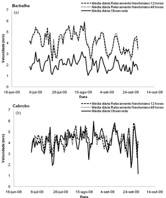
Figure 4-a presents the series of daily average wind speeds for simulated and observed data. It can be stated that varying the Newtonian relaxation time scale causes higher

bias errors in Barbalha/CE station, while the mean absolute and mean square errors also increase according to Table 4. There are low concordance indexes in this case, even though there are strong correlation coefficients in both time scales. It can be also seen that RAMS model presents better performance when configured with relaxation time of 12 h according to the presented methodology.

The results for Cabrobó/PE show that the simulated series follow the observed values (Fig. 4-b). According to Table 5, the highest weights for the statistical indexes occur when relaxation time scale of 12 h is considered for the sim-ulated data, thus providing the accurate representation of the wind regime in the study region.

3.3. Adjustment of the simulated series

wind fields in the study region. Although, the series of sim-ulated values presents bias and statistical errors, what

makes it diverge from the observed one. Therefore, once the goal is to approximate the simulated values to the

ob-Figura 4- Daily Average of wind speed simulated at 10 m high for the grade of 5 km for the quarter of July. August and September of 2009 for the locali-ties of Barbalha (a) and Cabrobo (b).

Tabela 5- Calculated Statistical Indexes. for the measurements of wind speed. for the model configurer with a Newtonian Relaxation time scale of 15 h (RN 12 h). And for a configuration of Newtonian Relaxation of 48 h (RN 48 h). in the locality of Barbalha and Cabrobó. The presented indexes are the sta-tistical bias (b). Mean Absolute Error (EAM). Mean Square Error (EQM). rate between Standard Deviation (R). Mean Absolute Error of the Deviations (EAMD). Mean Square Errors of the Deviations (EQMD). Concordance Index (Ic) and Correlation Index. The Total of Scores obtained by each variable are also shown.

Barbalha/CE b EAM EQM R EAMD EQMD Ic r Pesos

RN 12 h 2.11 2.11 2.19 0.59 0.47 0.56 0.34 0.77 11

RN 48 h 2.10 2.10 2.18 0.60 0.48 0.58 0.33 0.73 4

Cabrobó/PE

RN 12 h 0.16 0.53 0.69 1.16 0.51 0.67 0.78 0.63 12

gression comprehends the wind speed data obtained during July 2009 and August 2009. On the other hand, the valida-tion period aggregates the values corresponding to Septem-ber 2009. Once the curves are fitted, the statistical indexes for the adjusted series can be calculated.

The series of adjusted values have as a base the simu-lated values using the model configured with Mellor and Yamada’s parameterization and a Newtonian relaxation time scale of 12 h, since RAMS model has presented better performance when representing the wind speed fields in the investigated regions.

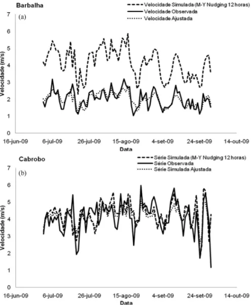
Figure 5 shows the series of simulated, observed and adjusted values by the linear regression method in the study regions. Table 5 presents the statistical indexes calculated

Newtonian relaxation time scale is 12 h.

Considering the comparison between the adjusted values and the obtained ones in the meteorological station of Barbalha/CE, it can be seen that curve fitting allows de-creasing the statistical bias between the series, and conse-quently higher values for the statistical correlation coeffi-cient (0.86) and the concordance index (0.89) could be obtained (Table 6).

The fitted curve for Cabrobó/PE causes the statistical bias to decrease, while a small increase occurs between the standard deviations. Besides, there is a slight decrease of the concordance index for the adjusted series if compared with the observed one (Table 6).

4. Conclusion

According to the obtained results, it can be concluded that the model is able to detect the variability tendency of the observed series of wind speeds in all the tested configu-rations, as the statistical correlation coefficient is classified from moderated to strong, with values higher than 0.5 in ev-ery case.

Considering the sensibility to the turbulence parame-terization where Mellor and Yamada’s and Smagorinsky’s schemes have been tested, the statistical analysis has shown that the first one presents better performance in the repre-sentation of wind speed fields.

Although values for the correlation coefficients could be classified from moderate to strong, the series of simu-lated values in the performed tests has presented apprecia-ble bias and statistical errors in some cases. This fact is evidenced by the differences between the curves in Figs. 3 and 4, which cause low values of concordance index.

The sensibility test to the Newtonian relaxation time scale has revealed slight differences between the simulated series with time scales of 12 and 48 h. In such cases, the simulated values overestimate the observed wind speeds in the stations, even though the series of simulated values seems to follow the variability tendency of the observed values graphically.

The statistical analysis has also demonstrated that the model configured with Newtonian relaxation time scale of 12 h is more accurate in the representation of the wind fields for two investigated regions because higher weights are assigned in this analysis.

Therefore, through the analysis of obtained results with sensibility tests performed using the RAMS model configured with the previously mentioned turbulence para-meterizations and Newtonian relaxation time scales, it can be stated that such regional model is able to represent the wind fields observed in the meteorological stations of Bra-calha/CE and Cabrobó/PE more accurately. For this pur-pose, Mellor and Yamada’s scheme (1974) and a Newto-nian relaxation time scale of 12 h are used. Such results are in accordance with the analysis carried out by Santiago de Maria (2008) and Oliveira and Costa (2011).

It can be also concluded that the application of the method proposed by Liraet al.(2011) for curve fitting pur-poses causes the statistical bias between the studied series to be reduced. This fact can be observed graphically in the presented curves, while the correlation coefficients

be-tween the series of adjusted and observed values are increased.

Finally, it is worth to mention that the analysis carried in this work evidences that the regional model RAMS can be used as an auxiliary tool in the prediction and planning for the energetic sector in SARNB, being able to assess po-tential sites for the installation of wind farms in agreement with the proposal of Martinset al.(2007).

References

ALCÂNTARA, C.R.; SOUZA, E.P. A thermodynamic theory for breezes: test using numerical simulations.Brazilian Jour-nal of Meteorology, v. 23, n. 1, p. 1-11, 2007.

ALVES, J.M.B.; BRISTOT, G.; COSTA, A.A.; MONCUNNIL, D.F.; SILVA, E.M.; SANTOS, A.C.S.; BARBOSA, W.L.; NÓBREGA, D.B.S.; SOUZA FILHO, V.P.; SOUZA, I.A. A technique applying downscaling dynamic in the northern sector of northeastern Brazil.Brazilian Journal of Meteo-rology, v. 18, n. 2. p. 161-180, 2003.

CHEN, C.; COTTON, W.R. The one-dimensional simulation of

the stratocumulus-capped mixed layer. Boundary-Layer

Meteorology, n. 25, p. 289-321, 1983.

COTTON, W.R.; ALEXANDER, G.D.; HERTENSTEIN, R.; WALKO, R.L.; McANELLY, R.L. Cloud venting - A re-view and some new global annual estimates.Earth-Science Reviews, v. 39, n. 3, p. 169-206, 1995.

CUADRA, S.V.; ROCK, R.P. Numerical simulation summer cli-mate on Brazil and its variability.Brazilian Journal of Me-teorology, v. 21, n. 2. p. 271-282, 2005.

DEVORE, D.L. Probability and statistics for engineering and sci-ence. São Paulo-Brazil: Thompson Learning Thomson Learning; 2006.

GOBBLE, J.L. Probability and Statistics for Engineering and Sci-ence. São Paulo: Thomson Learning. 702 p.

GOMES FILHO, M.F.; GALVÃO, C.O.; RICARTE, R.M.; SIL-VA, M.C.L.; BRIDGES, A. L.; BECKER, C.T. Convective systems Mesoscale with heavy precipitation in Paraíba: a case study.Brazilian Journal of Meteorology, v. 11, n. 1, p. 36-43, 1996.

KUO, H-L. Further studies of the parameterization of the influ-ence of cumulus convection on large-scale flow.Journal of the Atmospheric Sciences, v. 31, n. 5, p. 1232-1240, 1974.

LIMA, J.P.R.; ALVES, J.M.B. A study of dynamic downscaling of intraseasonal rainfall coupled to rainfall-runoff model in the upper-middle basin San Francisco.Brazilian Journal of Meteorology, v. 24, n. 3, p. 323-338, 2009.

LIRA, M.A.T.; SILVA, E.M.; ALVES, J.M.B. Estimation of wind resources in Ceará using the theory of linear

regres-sion. Brazilian Journal of Meteorology, v. 26, n. 3,

p. 349-366, 2011.

Tabela 6- Calculated statistical indexes. for the simulated and previewd by linear regression wind speed. in the locality of Barbalha. The presented in-dexes are the statistical bias (b). Mean Absolute Error (EAM). Mean Square Error (EQM). rate between Standard Deviation (R). Mean Absolute Error of the Deviations (EAMD). Mean Square Errors of the Deviations (EQMD). Concordance Index (Ic) and Correlation Index. The Total of Scores obtained by each variable are also shown.

b EAM EQM R EAMD EQMD Ic r

Barbalha/CE -0.07 0.20 0.24 1.35 0.20 0.23 0.89 0.86

wind energy. Journal of Physics Teaching, v. 30, n. 1, p. 1304, 2007.

MELLOR, G.L.; YAMADA, T. A hierarchy of turbulence closure models for planetary boundary layers.Journal of the At-mospheric Sciences, v. 31, n. 7, p. 1791-1806, 1974. MELO, M.L.D.; MARENGO, J.A. Middle Holocene climate

sim-ulations in South America with the general circulation model of the atmosphere of the CPTEC.Brazilian Journal of Meteorology, v. 23, n. 2, p. 190-204, 2007.

MENEZES NETO, O.L.; COSTA, A.A.; RAMALHO, F.P. Esti-mation of solar radiation via mesoscale atmospheric model-ing applied to northeastern Brazil. Brazilian Journal of Meteorology, v. 24, n. 3, 339-345, 2009.

OLIVEIRA, J.L.; COSTA, A.A. Wind Variability Study on sea-sonal scale over northeastern Brazil using the RAMS: cases of 1973-1974 and 1982-1983.Brazilian Journal of Meteo-rology, v. 26, p. 53-66, 2011.

PIELKE, R.A.; COTTON, W.R.; WALKO, R.L.; TREMBACK, C.J.; LYONS, W.A.; GRASSO, L.D.; NIEHOLLS, M.E.; MORAN, M.D.; WESLEY, D.A.; LEE, T.J.; COPELAND, J.H. A comprehensive Meteorological Modeling System

-RAMS. Meteorology and Atmospheric Physics, v. 49,

n. 1, p. 69-91, 1992.

PIELKE, R.A.; COTTON, W.R.; WALKO, R.L.; TREMBACK, C.J.; LYONS, W.A.; GRASSO, L.D.; NICHOLLS, M.E.;

Numerical modeling for high resolution prediction for wind power generation in Ceara.Brazilian Journal of Meteorol-ogy, v. 23, n. 3, p. 477-489, 2008.

SILVA, B.B.; ALVES, J.A.J.; CAVALCANTI, E.P.; VENTU-RA, E.D. Spatial and temporal variability of the wind poten-tial of the prevailing wind direction in northeast Brazil. Bra-zilian Journal of Meteorology, v. 19, n. 2, p. 189-202, 2004.

SMAGORINSKY, J. General circulation experiments with the

primitive equations: I. The basic experiment. Monthly

Weather Review, v. 91, n. 3, p. 99-164, 1963.

SOUZA, E.P.; SILVA, E.M. Impact of implementation of a shal-low convection parameterization in a mesoscale model. De-scription and scheme of susceptibility testing. Brazilian Journal of Meteorology, v. 18, n. 1, p. 33-42, June 2003.

WALKO, R.L.; TREMBACK, C.J.; BELL, M.J.H.Hybrid

parti-cle and concentration transport model. User’s guide, p. 80525-0466, 2001.

XAVIER, T.M.B.S.; XAVIER, A.F.S.; DIAS, P.L.S.; DIAS, M.A.F.S. The intertropical convergence zone - ITCZ and its relations with rain in Ceará (1964-98).Brazilian Journal of Meteorology, v. 15, n. 1, p. 27-43, 2000.