CERNE
Historic: Received 08/12/2017 Accepted 13/03/2018
Keywords: El-Nino La-Nina Forecast Co-integration SARIMA
1 Federal University of Uberlândia - Uberlândia/Monte Carmelo, MInas Gerais, Brazil, ORCID: 0000-0003-4542-0933 2 Federal University of Uberlândia - Uberlândia, MInas Gerais, Brazil, ORCID: 0000-0001-9651-9533
3 Federal University of Uberlândia - Uberlândia, MInas Gerais, Brazil, ORCID: 0000-0002-5497-5159 4 Federal University of Uberlândia - Uberlândia, MInas Gerais, Brazil, ORCID: 0000-0001-5213-2070
+
Correspondence: [email protected]
DOI: 10.1590/01047760201824012487
Claudionor Ribeiro da Silva1+, Sérgio Luís Dias Machado2, Aracy Alves de Araújo3, Carlos Alberto Matias de Abreu Junior4
ANALYSIS OF THE PHENOLOGY DYNAMICS OF BRAZILIAN CAATINGA SPECIES WITH NDVI TIME SERIES
SILVA, C. R.; MACHADO, S. L. D.; ARAÚJO, A. A.; ABREU JUNIOR, C. A. M. Analysis of the phenology dynamics of brazilian caatinga species with NDVI time series. CERNE, v. 24, n. 1, p. 48-58, 2018.
HIGHLIGHTS
The generation of time series of NDVI and Surface temperature generated from digital images (Landsat) that are available for free;
To present a detailed study about the Caatinga, which goes through a period of serious environmental degradation;
Promote prediction of vegetative behavior in at least one year, to subsidize the public and private bodies responsible for preserving this Biome in actions and decision-making;
Provide another study on the Caatinga, which is a biome that still lacks detailed studies.
ABSTRACT
In Brazil there are six well-defined biomes and the Caatinga represents 9.92% of the
total area. This biome is exclusively Brazilian and very rich in biodiversity. Because it has low resistance to human interference is necessary to know the important factors in monitoring the biome. Vegetation coverage and climate are two of these factors, as they indicate the intensity of human activity and the wear caused with time. Normalized Difference Vegetation Index (NDVI) has been recently explored in the description of tree phenology. In this study we sought to associate NDVI/Landsat values to a climatic variable (phenomena El-Nino and La-Nina - NINONINA) in order to describe the phenological behavior of the Caatinga in the Parque Nacional da Serra das Capivaras in the state of Piauí/Brazil. A time series analysis was carried out, describing the intrinsic parameters of the series (Seasonality and Trends), the forecast of NDVI values using SARIMA model and co-integration between NDVI and NINONINA series. The results showed that the NDVI series presents seasonally, but does not exhibit a trend. The forecasting process
presenting relatively low error at a 95% confidence interval. Finally, it was observed that
INTRODUCTION
Brazil has an enormous land area, approximately 8,500,000 km2, where you can verify very diverse weather, soils and vegetation coverage. Throughout the length of the country there are portions with similar
characteristics and continuous biodiversity, which defines
the so-called “biomes”. A biome is understood as a set of all living beings in a region that presents uniformity and a common history in its formation. There are six
well-defined biomes in Brazil (% in area): Amazon (49,29%), Cerrado (23,92%), Atlantic Forest (13,04%), Caatinga (9,92%), Pampa (2,07%) and Pantanal (1,76%) (IBGE,
2016). The Caatinga is an exclusively Brazilian biome.
Etymologically, the term Caatinga (Tupi-Guarani) means
white forest. This name stems from the whitened landscape, characterized by the appearance of the tree trunks in the dry season due to the almost total loss of
foliage. Nearly 10% of the national territory, occupied
by the Caatinga, encompasses part of the states of
Alagoas, Bahia, Ceará, Maranhão, Minas Gerais, Paraíba, Pernambuco, Piauí, Rio Grande do Norte and Sergipe.
Studies indicate that the Caatinga came about with the extinction of existing tropical forest in the area, which occurred at the end of the ice age, ten thousand years ago. These studies show that the Caatinga is heterogeneous, being very rich in biodiversity and endemic species.
Caatinga vegetation is classified as steppe savanna and
the landscape is quite different due to the sharp variation of rainfall, fertility and types of soil and topography. The particularity of the vegetation coverage of the Caatinga
allows for the classification of the landscape into two
distinct types: agreste (wild harsh lands) and sertão
(hinterlands). The first involves the transition between the dry area and the Atlantic Forest, which is dominated by
shrubby trees, with many interwoven branches; and the second (sertão/hinterlands) has more rustic vegetation. Despite its great wealth in biodiversity, the Caatinga is the most fragile Brazilian biome. The indiscriminate use of soil and natural resources, during the occupation/ exploitation process, has degraded the Caatinga. The uniqueness, fragility, unsustainable use, particular wealth and small extent express the need for studies which seek to preserve the biome (Leal et al., 2005).
One of the first major events open to discuss
global environmental issues was held in Stockholm (United Nations Conference on Environment) in 1972. However, it is only recently that research addressing environmental issues has gained highlights, especially due to the phenomena causing environmental degradation, environmental policy and the principles of environmental sustainability, with the purpose of seeking partial or total solutions for the problem (Almeida et al., 2012).
Originally, natural environments present themselves in a state of dynamic equilibrium, which is destabilized by anthropogenic actions (ROSS, 1994). The indiscriminate exploitation of exhaustible natural resources (such as water, soil, air, vegetation and minerals), for example, provides a serious environmental wear/deterioration, reaching irreversible cases. Land use change, particularly in a forested ecosystem, has a direct impact on the global carbon cycle. Consequently, the regional assessment of biomass and the understanding of its current spatial controls are research priorities
for regional ecology and land use (GASPARRI; BALDI,
2013). The Caatinga, being a fragile biome, has no strong resistance to such actions, being exposed to degradation
phenomena such as desertification. Depending on
the severity of the degradation, these resources are unavailable in quantity and/or in quality. In this context, given the particularity of the biome, it is necessary to know the factors that can contribute to the management, planning, handling and environmental monitoring locally, so as to establish a parallel between the exploitation of natural resources and the complex technological,
scientific and economic development of the country.
Vegetation coverage and climate are two fundamental elements in the study of environmental degradation behavior, as they indicate the intensity of human activity and wear over time. An extensively explored parameter for the analysis of vegetation coverage is the Normalized Difference Vegetation Index (NDVI) calculated with the use of digital images, more
specifically, the red and infrared bands of a multi-spectral
sensor. This index is a numerical indicator of the intensity of the presence of vegetation, ranging from [-1 +1], indicating with -1 (minus one) the absence of vegetation (low or nil chlorophyll content) and 1 (one), the presence of vegetation in its chlorophyll plenitude. Recently some studies have been made in order to show the applicability of NDVI values to describe the behavior of different plant vegetation types. In most of these studies low spatial resolution data are used, such as data from MODIS/NOAA satellites, or adjusted data NOAA/MODIS/Landsat (JIA, 2014; PINZON; TUCKER, 2014; LAMBERT et al., 2015). In addition to the NDVI (vegetation coverage), weather data are also important in the process of environmental degradation. The El-Nino and
La-Nina phenomena are climatic parameters that reflect the
series (trend, cycle, seasonality) are analyzed, as well as a prediction of their behavior being modeled. In addition, the co-integration between the series “NDVI” and “Climate” is analyzed, pointing out the interference of the weather in the variation of chlorophyll content of Caatinga vegetation. Knowledge of time series
elements allows for the identifi cation and understanding
of standards and ecological and evolutionary processes
that operate in the Caatinga. Given that the Caatinga
is the biome which is proportionately less studied and less protected in the country, the results of this research become important contributions to the elaboration of the management plan of the species in the region, avoiding problems such as the loss of unique species and
the formation of desertifi cation centers.
MATERIAL AND METHODS
Study Area
Study area is the Serra da Capivara National Park (PARNASC), which has 91,848.88 ha of protected area in the Southeast of Piauí State, in northeastern
Brazil (Figure 1). This area includes part of the
Municipalities of: São Raimundo Nonato, Coronel José Dias, Brejo do Piauí and João Costa. The PARNASC is bounded by the geographical coordinates (Datum:
SIRGAS2000): ( =08º30’00” S, =42º45’39,25” W) and ( =08º50’5,55” S, =42º19’15,14” W). It has a semi-arid climate and covers part of the sandstone plateau, dominated by tree-shrub Caatinga (location chosen for sampling-pixels). There are canyons in the area that contain enclaves of semi-deciduous forest and a rupicolous vegetation characteristic, displayed in
exposed fl agstones. The valleys of PARNASC are home
to Caatinga trees larger than 15 meters (Emperaire,
1989; Fumdham, 2016; Ribeiro-Neto et al., 2016).
In the Caatinga the average annual temperatures are high (25º-29ºC) with high solar radiation. The climate is semi-arid, mainly resulting from the predominance of stable air masses, pushed by the southeast trade winds, which have their origin in the South Atlantic anticyclone action. Consequently there is a low relative humidity rate and very high evapotranspiration potential. The soil which is derived from different types of rock is still shallow and stony. Droughts are cyclical and prolonged. The rainy season is short, starting at the beginning of the year and with lower and irregular rainfall. The occurrence
of catastrophic phenomena such as droughts and fl oods
are very common (Leal et al., 2003; Silva et al., 2016).
The Government has sought economic
development in the region, but always comes up against the problem of soil aridity and the instability of
rainfall. Farming is the main economic activity carried
out in Caatinga. The region has social problems such as low levels of income and schooling and high infant mortality rate. Some irrigation projects for agriculture
are developed in the valleys of the São Francisco and
Parnaíba rivers, which are the main rivers of the region
(Leal et al., 2005; Francisco, 2016).
Datasets
Due to the long running Landsat 5 (Thematic Mapper sensor - TM) we chose to use the images from this satellite, for generation of NDVI time series. However, due to a problem which occurred with the supply of images from Landsat 5, in 2002, images from Landsat 7 ETM + were used for that year. Although both the TM sensor and the ETM + generate 7 spectral bands (electromagnetic spectrum), this study used only bands 2 (green: 0.52-0.60 m), 3 (red: 0.63-0.69 m) and 4 (near infrared: 0.76-0.90 m). This trio of bands was collected monthly during the period from 1984 to 2010. The spatial resolution for these bands is 30 meters. All Landsat 5 TM and Landsat 7 ETM+ images were obtained free on
the site/web United States Geological Survey (USGS) in:
http://landsat.usgs.gov/landsat8.php.
The occurrence of the climatic phenomenon (El Niño and La Niña) is represented by indexes in quarterly
values. The fi rst index is JFM: January, February and March; second is FMA: February, March and April; third
is MAM: March, April and May, and so on. This index is based on the limit of ±0.5°C for the anomalous temperature at the sea surface (SST) in the Niño 3.4 region (5°N to 5°S latitude and 120°W 170°W longitude). The positive index refers to El Niño and negative for La FIGURE 1 Location of the Caatinga and the Serra da Capivara
Niña. These indexes were obtained free in: http://www. cpc.ncep.noaa.gov/ (Silva et al., 2011).
The ENVI 4.8 software image processing (Exelis Visual Information Solutions) is used to images preprocessing and to determine NDVI. The processing
of the temporal series was carried out using free
Gretl-2016c software.
Generation of NDVI and NINONINA Time Series
As the two sensors TM/ETM+ of the Landsat series are identical, it was not necessary to make adjustments in the NDVI values of one sensor in relation to the other. In addition, before the NDVI calculation
all images had been previously recorded (fi rst degree
polynomial model) so as to ensure the geometric consistency between the corresponding pixels of images
from different dates. For the recording of the images the
oldest image of 1984 was used as reference. Band 2 of the TM/ETM+ sensor was used only at that stage, so as to generate a color image, which facilitates the collection of the control points to record the scenes. Still in the preprocessing phase, all Landsat images were corrected for atmospheric effects. All of these preprocessing procedures were performed in the ENVI 4.8 software.
In the fi rst step of the processing, the NDVI was
calculated in all images used. The NDVI was selected
because of its effi ciency in recording the phenological
changes in vegetation (RAO et al., 2015). The method is widely recognized in literature and uses simple arithmetic calculations of spectral bands (Equation 1), where R and
IR are the red spectral and infrared bands, respectively.
Subsequently, in each NDVI image, the digital value of the pixel in the same geographic location, or the digital value of another pixel very close to it, was collected and stored in the form of a column vector forming the monthly NDVI time series. In this vector, the
fi rst twelve cells store the NDVI values of the fi rst year
(1984), in the order from January to December. The next twelve values refer to the subsequent year (1985), and so on. Storing in a vector shape is to facilitate entry of the
time series in the Gretl software.
Although the region presents characteristics of prolonged drought, in some years there are periods with heavy rainfall, resulting in images covered by many
clouds. This fact occurs in specifi c months, usually
from December to March. This problem was resolved [1]
in two ways: a) when the month before or after the month with clouds had two scenes, one was used for this problematic month; and b) when the previous case did not occurred, the NDVI values were interpolated by the kriging method. Kriging was chosen because it is an interpolation method already established in literature. There were few interpolated values. The time series is monthly and corresponding to a period of 27 years, 1984-2010.
The second time series, referring to the climatic phenomenon was easily stored in the same manner as the column vector, presenting the same size of NDVI vector. As shown in Silva et al. (2011), the quarterly values of the indices corresponding to the occurrence of El Niño and La Niña describe the behavior of these phenomena over time. Each year is punctuated by twelve quarters which overlap each other, for example,
DJF (December, January and February) is the fi rst
quarter, representing the month of January; the second
is JFM (January, February and March), representing the month of February, and so on. This index is based on
the limit of ±0.5°C for the anomalous temperature at the sea surface (SST) in the Niño 3.4 region (5°N to 5°S latitude and 120°W 170°W longitude). Positive values of this index show the occurrence of El Niño and negative values indicate the occurrence of La Niña. The values of the El Niño and La Niña indexes were obtained free of charge at: http://www.cpc.ncep.noaa.gov/.
Processing the NDVI and NINONINA Time Series
The processing of the NDVI and Climate (NinoNina) time series was used to evaluate the behavior
of the Caatinga vegetation covering over time. For this
purpose the functions of the package “time series” of the
Gretl-2016c software were used. This phase was divided
into three steps: a) analysis of the parameters/basic elements of the time series; b) analysis of NDVI series forecast and c) analysis of co-integration of the NDVI and NINONINA series.
Analysis of the basic elements of the NDVI and NINONINA time series
variables, events or phenomena in an interval of time after that observed. Before the calculation of the forecast it is necessary to carry out some tests in the series so as to verify the applicability as well as identifying features such as the stationarity of this series.
by means of Equation 5, where µ_t is the white noise term; and δ is the indicator where, if δ=0, the series does not have a unit root and the variable ∆Yt becomes equal to the white noise, which is by its very nature stationary. This
means that the fi rst differences of a time series of a random
walk are stationary (Enders, 1995). [2]
[3]
The trend expresses the long-term behavior and shows changes that occur in the average level of the series which may be deterministic (mathematical model) or stochastic (random process). The trend can be used both for predicting future values of the series and to assess the seasonal component.
Irregular variations are changes which were not foreseen in relation to the trend line, resulting from
unexpected events such as a fi re or deforestation in the
case of NDVI series, commonly referred to as white noise.
Cyclical or cycle variations are fl uctuations in the
form of long waves that occur around the trend line, referring to the values of variables, events or phenomena, and which repeat over time. These cycles allow for the detection of changes occurring in the series, such as
infl ection point, duration and frequency.
Seasonal variations are cyclical movements that are completed during a period and reproduce themselves
in other similar periods, defi ning regular patterns of the
series. In the study of a time series it is important that the
seasonal component be identifi ed and isolated so that it
can work with a deseasonalized series (free or seasonally adjusted). The deseasonalization process is based on Equation 4, where
adjusted). The deseasonalization process is based on is an estimate of the seasonality (St ) of the series.
[4]
There are several tests for analysis as to the existence of a unitary root. Analysis by means of correlogram, for example, is a straightforward and easy test to be interpreted. Another test which is widely used to test the δ coeffi cient signifi cance (there is unitary root) is the Augmented Dickey-Fuller (ADF) test. In this
test, if the null hypothesis Ho:δ=0 is rejected, the data series does not have a unitary root, in other words it is stationary. When the data series has unitary roots, it
is common to test if the fi rst differences are also
non-stationary, as shown in Equation 6, where β is the intercept and α_i is the regression coeffi cient.
[5]
[6]
Both time series (NDVI and Climate) will be analyzed in relation to their basic elements: trend (T), seasonal (S), cycle (C) and irregular variations (I), if any.
The ADF test will be applied in both series to verify the
existence of stationarity or not.
Forecast analysis of NDVI series
The autoregressive models which are integrated with a moving average (ARIMA) are widely used to forecast data using time series, especially because they are also used in non-stationary series. Such models are based on the theory that a variable Yt can be explained by the historical values of this variable itself, added to the stochastic error terms of the series.
Considering that the Yt time series is stationary with the application of d differences, the ARIMA model for prediction is given by Equation 7 (Enders, 1995).
Knowing the coeffi cients and , a prediction Yt+1 can be made by Et Yt+j= + Yt, in which the
fi rst term is the conditional expectation of Yt+j, given the
available information as to t. For other predictions in
periods 2, 3, ... j, use Equations 7 and 8. In a stochastic time series it is necessary to know
whether the randomness of the variables do not change in time, which characterizes a stationary process. In this way, a stochastic time series is said to be stationary when presenting average and constant variance in time and the covariance between two periods depends only on the distance or the gap between the two periods, and not on the effective time period in which the covariance is calculated (Box et al., 2015;
Gujarati, 2009; Enders, 1995).
The stationarity of a time series can be obtained by unit root tests. Considering the regression of the values of variable Yt on its out of date values Yt-1, obtained
[7]
trend variable and making an OLS regression. It was
verified that the time variable added to the model was not statistically significant. In addition to this test two
other experiments were also made to check the trend: one with the square of the time variable, previously created and another with the logarithm of the NDVI variable. In both cases it was also found that the series showed no trend.
The forecast for the NDVI series will be carried
out in two stages. In the first stage, the year 2010 will be
removed from the series for the 12-month forecast error analysis. In the second stage the year 2010 will be reinserted and the forecast will be determined for the year 2011.
Co-integration analysis between the NDVI and NINONINA series
To check if there is a long term equilibrium relationship between NDVI and NINONINA series, a co-integration analysis will be carried out between the two variables. The co-integration analysis can be performed
by the models proposed by Engle and Granger (1987) and Johansen (1988). In Engle and Granger (1987) model the integration order of the variables must be tested first; if
the order is the same, continue the test, otherwise, the variables are not co-integrated. If integration is zero order, there is no reason to test for co-integration. In this case, one must estimate a regression of Ordinary Least Squares (OLS) and test waste stationarity by using a test such as
Dickey-Fuller, Dickey-Fuller increased or Durbin-Watson.
RESULTS
Trend and Seasonality and Stationarity of NDVI Series
The analyzed series NDVI and NINONINA have 324 observations, covering the time period from January
1984 to December 2010. First of all, a graphic display was performed (Figure 2) of the data relating to the two
series, so as to perform an analysis of its basic elements.
By observing the graphs of the two series, we find that there are no outliers and not even a definite trend.
On the other hand, a possible seasonality is revealed on the NDVI series graph because of the uniform behavior
in the form of waves. To confirm the visual analysis,
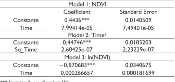
we proceeded to the trend and seasonality tests. The NDVI series, as shown in Table 1, did not really present a tendency. The test was carried out by adding a time
FIGURE 2 Location of the Graphical representation of NDVI and NINONINA series.
TABLE 1 Analysis of the trend of the NDVI series. Model 1: NDVI
Coefficient Standard Error Constante 0,4436*** 0,0140509
Time 7,99414e-05 7,49401e-05 Model 2: Time²
Constante 0,44746*** 0,0105203 Sq_Time 2,60425e-07 2,23229e-07
Model 3: ln(NDVI)
Constante −0,870683*** 0,0340675 Time 0,000266657 0,000181699
*** Statistically significant at 1%.
a.
b.
FIGURE 3 Periodogram of NDVI series spectrum: a) modeled; b) with seasonal component.
Based on the graph/periodogram (Figure 3a) the
presence of seasonality was observed. Then we tried to model this seasonality by seasonal lag. The seasonal effect
After the identifi cation of the seasonal component, the
correlogram test to identify the presence of a unit root
and the Augmented Dickey-Fuller test (ADF) in order to
identify if the time series in question is stationary were applied, in other words, if it does not have root unit. The results showed that the NDVI series is not stationary, as
the p-value calculated was > 5%, so it was not possible
to reject the null hypothesis (the series has a unit root). In order to make the series “stationary”, differentiations were made in series and once again the tests were carried
out. For the ADF test, after the second difference, a p-value <5% was obtained, demonstrating that the series was stationary. In addition to the ADF test, the correlogram analysis also confi rmed that the series has
become stationary.
Based on the defi nition of the stationarity order of the NDVI series the identifi cation of the autocorrelation fi lter (RA) and the median fi lter (MA) were made. Accordingly,
after analyzing the autocorrelation the estimated model is a SARIMA (1,2,2) x (0,1,2), whose result of the estimation is shown in Table 2.
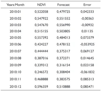
Based on Figure 4 it can be seen that the forecasted values are within the signifi cance areas and
are very close to the actual values of 2010. The actual and forecasted values, as well as the difference (error) between these values are shown in Table 3.
The reliability of the forecasting method used is guaranteed by the low value of the mean square error (0,00285) and by the modest value of the standard
deviation error (0,05036). Once confi rming the accuracy
of the forecasting method of NDVI values, the forecast was made for the year 2011, using all the NDVI (1984-2010) series. The forecasted values for 2011 are plotted
in Figure 5.
The predicted values (Figure 5) indicate
that there is a good adjustment of the forecast on a
confi dence interval of 95%. It is noticed that the
behavior of the NDVI series is consistent with the values of previous years.
TABLE 2 SARIMA Model (1,2,2)x(0,1,2).
Coeffi cient Standard Error
0,3587*** 0,0598
_1 -1,9305*** 0,0250
_2 0,9308*** 0,0250
Θ_1 -0,8571*** 0,0351
Θ_2 -0,0481*** 0,0183
*** Statistically signifi cant at 1%
TABLE 3 Actual and forecasted values of the NDVI series in 2010.
Years:Month NDVI Forecast Error
2010:01 0,522058 0,479725 0,042333
2010:02 0,547922 0,551552 -0,00363
2010:03 0,547670 0,556990 -0,00932
2010:04 0,515155 0,503805 0,01135
2010:05 0,557392 0,484013 0,073379
2010:06 0,424227 0,478152 -0,053925
2010:07 0,444444 0,375317 0,069127
2010:08 0,387016 0,372371 0,014645
2010:09 0,339312 0,316154 0,023158
2010:10 0,246572 0,308404 -0,061832
2010:11 0,468888 0,383575 0,085313
2010:12 0,596359 0,510888 0,085471 It is observed that all the variables of the estimated
model (Table 2) were signifi cant at 1% in the formulation
of the SARIMA model (1,2,2)x(0,1,2).
Forecast of the NDVI Series
The good specifi cation of the model, together
with the fact that the series became stationary, guarantees the forecast of the series in a safe manner. The forecast was made in two stages: a) the forecast for the year 2010, with the series reduced for the 1984-2009 period
(Figure 4); and b) the forecast for the year 2011, with all the values of the series (1984-2010). In the fi rst case, the
objective is to compare the forecasted values with the actual values of the NDVI series, recorded in the year
2010. Figure 4 presents both graphs, that of forecast and
real values.
Co-integration of the NDVI and NINONINA Series
After analyzing the NDVI series we preceded with the analysis in the same manner and parameters for the NINONINA series. The NINONINA series showed no
trend and no seasonality and the stationarity test (ADF)
showed that the series has become stationary after the
second differentiation, with a confidence level of 95%.
Subsequently, the co-integration test was carried out to check if there is a long-term equilibrium relationship between the two variables (NDVI x NINONINA). That is, verify if the series can move together in time and if the difference between them is stable (stationary).
To identify the presence of co-integration between
the two series, the Engle-Granger test was used. As
already mentioned above, the series are stationary with 2 lags, leading only to the need to check whether the waste of co-integration equation is stationary. By means
of the Engle-Granger test it was found that residues from
the co-integration regression are stationary, indicating that the two series are co-integrated.
Given that the two series are co-integrated, it
was possible to calculate the error correction vector based on the residues from the co-integration equation. After graphical analysis it was found that the residues have no tendency and can continue with the correction mechanism, since, when co-integration is observed, it
is confirmed that there is long term equilibrium ratio,
however the same is not true for the short term. By analyzing the error correction vector (0,02313) in the model having NINONINA as the dependent
variable, it is found that the same was significant,
indicating that the NINONINA series responds to the imbalance between both NINONINA and NDVI.
DISCUSSION
In Dong et al. (2015) is reported that the Landsat has become a major data source for people to conduct FIGURE 5 Forecast graph of the NDVI series for the year 2011.
time series image analysis. The sensors TM/ETM provides information at a higher spatial resolution (30m) and longer temporal range (since 1970s). However, there is no continuous series, because there are many images
covered by clouds and interpolation is required to fill the time series. In Fisher et al. (2006) is advised that it should
be aware that additional weight given to the bounding
points which guide the interpolation will be reflected in the final product. In this context, to validate the kriging
interpolation, several experiments were performed, validating the interpolation and real NDVI data taken from the series. In these experiments, the greatest differences between actual and interpolated values were 0.02, which is an acceptable value for the study.
The presence of the seasonal component in the NDVI time series was expected, since the intensity of the chlorophyll and foliage of the Caatinga tree species usually varies with the changes of the seasons, repeating each year. The analysis of the periodogram of the NDVI series made this premise clear by pointing individualized peaks, which represents the seasonality. Disregarding this parameter can cause losses in the results, as pointed out by Nassur et al. (2015).
The original NDVI series proved to be non-stationary. According to Diniz et al. (2016), seasonal time series or with linear or exponential trend are examples of time series with non-stationary behavior, which agrees with the result found in this study. However, most statistical procedures of time series assumes that the series are stationary, otherwise the original data must be transformed. In this study, the NDVI series was subjected to a lag, which was enough to make it stationary.
The NDVI forecast for the year 2010 showed that the method is effective, presenting a relatively low error. This reliable result allowed to determine the forecast for the year 2011, period without original data,
obtaining a satisfactory result in a confidence interval of 1%. It is worth noting that the prediction obtained in
this study corresponds to a period of one year, relatively long period, when compared to another study, which restricted the forecast in a few days (Nassur et al., 2015; Alhamad et al., 2007).
According to Gao et al (2017), phenology mapping
allows regionally monitor crop progress and condition
benefiting both crop management and production
benefits complementary to those discussed in Gao et al.
(2017), as the forecast of future production. Although not
detailed by Gao et al. (2017), the phenology dynamics
prediction technique is a primordial measure for the study of vegetation cover, important for the control and management in protected areas, because it allows controlling/avoiding the smooth and abrupt variations, such as the occurrence of pest or burn, respectively. Another important factor in this study is the use of similar sensor data (Landsat TM and ETM +) which avoids errors between different sensors; although there are approximations in the interpolation task used in this work.
Although this study analyzes the relationship
between NDVI and NINONINA, Fisher et al. (2006)
suggest topographic, coastal, and land-use controls
on phenology, since microclimates can influence the
onset of leaf growth and is of crucial importance in the interpretation of records in situ and in phenology interpolation from satellite data. The biome studied in this research meets these premises, because the Caatinga
is located in a region with a well-defined climate and is
at plateau, where the topographic variation is minimal. The changes in the NINONINA series cause variations in NDVI date. According to Barreto et al. (1996), the impact of the El Niño / La Niña in northeastern Brazil can only be assumed to date. However, based on the results obtained in this study, it can be said that this phenomenon is directly responsible for the plant health of the Caatinga. This means that long periods of El Niño can cause the degradation of the vegetation Biome, because this phenomenon is indicative of drier climates and consequently causes the reduction of the green value intensity (biomass), which leaves the most sensitive
region to fires and desertification.
The time series of vegetation index is often far from a simple pattern because environmental factors, mainly temperature and precipitation, control vegetation growth under natural conditions (Cao et al, 2015). According to these authors, the effect of temperature is smoother, while precipitation events are often temporarily unpredictable, directly affecting vegetation growth. The results obtained in the present study corroborate with the research by Cao
et al. (2015) which verified that precipitation has a strong
relationship with vegetation index and vegetation growth.
For these authors, the temperature affects vegetation
index more smoothly when compared to precipitation. In this sense, since NINONINA is directly related to the precipitation and temperature of a particular site it can to agree with the existence of cointegration of this phenomenon with the Caatinga NDVI, as pointed out in the results of this research.
For future work it is recommended to test new
interpolation methods to verify the quality of interpolated NDVI values. In the case of Caatinga, kriging method presented a good result, but for another biome or crop (vegetal cover) it may not be adequate.
CONCLUSIONS
According to Fisher et al. (2006), remote sensing
phenological models have been produced at coarse scales, ranging from kilometers (MODIS and AVHRR sensors). However, the Landsat TM and ETM+ data at 30m resolution has been used to classify the phenological behavior of agricultural crops over the course of a season and estimate productivity in forest stands. This motivated our study with the use of 26-year record (1984-2010) of Landsat 5TM and 7ETM+ data to model Caatinga forest phenologies in Brazil.
Different from this research, most of the studies carried out with a time series of vegetation index do not analyze the intrinsic parameters of the series, such as trend, seasonality, prediction, or even cointegration between series. In addition, many researches address the study of agricultural crop series, without an emphasis on
a particular biome (Dong et al., 2015; Gao et al., 2017;
Cao et al., 2015; Zheng et al., 2016).
The NDVI values relating to the Caatinga showed that when analyzed over time they are seasonal, but show no tendency. The results showed that it is possible to isolate the seasonality of the series for subsequent calculation of parameters such as forecasting and co-integration with other series.
The model used to forecast (SARIMA) was
shown to be efficient and with relatively low error. This
result is very important in the monitoring, management and recovery processes of areas of the Caatinga, as it indicates the health condition of the vegetation over the coming year. This information is an important aid for the governing body of the Conservation Unit under study, for planning actions focused on local biodiversity.
The results showed that the NDVI series is co-integrated with the NINONINA series. This co-integration points out the interference of the NINONINA phenomenon in the variation of chlorophyll content of the Caatinga vegetation. This factor may be useful in the absence of NDVI Caatinga data, as it will be possible to infer as to environmental actions based on NINONINA data.
The results show that the detailed spatial and temporal variability in Caatinga vegetation development
can be identified using interpolated Landsat TM and
ACKNOWLEDGMENTS
Minas Gerais State Research Foundation (FAPEMIG) is the agency for the induction and promotion of research and scientific and technological innovation in the State of Minas Gerais/Brazil. We thank FAPEMIG for the financial support given to our scientific project.
REFERENCES
ALHAMAD, M.N.; STUTHT, J.; VANNUCCI, M. Biophysical modelling and NDVI time series to project near-term forage supply: spectral analysis aided by wavelet denoising and ARIMA modelling. International Journal of Remote Sensing. v.28, p.2513-2548, 2007.
ALMEIDA, O.S.; MACEDO, D.F.; SANTOS, V.C.; ANJOS, K.F.
Environmental Education and Educational Practice: Study
In a State School of Divisa Alegre, Minas Gerais, Brazil.
Revista Metáfora Educacional. v.13, p.155-173, 2012.
BARRETO, A.M.F.; PESSENDA, L.C.R.; SUGUIO, K. Probable
drier Holocene climate evidenced by charcoal bearing middle
São Francisco River paleodunes, State of Bahia, Brazil. Anais
da Academia Brasileira de Ciências. v.68, p.43-48, 1996.
BOX, G.E.P.; JENKINS, G.M.; REINSEL, G.C. Time Series Analysis – Forecasting and Control. 5th ed.; John Wiley &
Sons: New Jersey, US. 2015. p.712.
CAO, R.; CHEN, J.; SHEND, M.; TANGA, Y. An improved
logistic method for detecting spring vegetation phenology in grasslands from MODIS EVI time-series data. Agricultural
and Forest Meteorology. v.200, p.9-20, 2015.
DINIZ, H.; ANDRADE, L.C.M.; CARVALHO, A.C.P.L.F.; ANDRADE, M.G. Previsão de séries temporais utilizando redes neurais artificiais e modelos de box e jenkins. Available
at: http://repository.usp.br/single.php?_id=000999625. Accessed in: 26 june 2016.
DONG, J.; XIAO, X.; KOU, W.; QIN, Y.; ZHANG, G.; LI, L.; JIN, C.; ZHOU, Y.; WANG, J.; BIRADAR, C.; LIU, J.;
MOORE, B. Tracking the dynamics of paddy rice planting area in 1986–2010 through time series Landsat images and phenology-based algorithms. Remote Sensing of Environment. v.160, p.99-113, 2015.
EMPERAIRE, L. Végetation et gestion des resources naturelles dans la caatinga du sud-est du Piauí (Brésil). 1989. Doctorat d’Etat ès Sciences Naturelles. Université Pierre et Marie Curie, Paris.
ENDERS, W. Applied econometric time series. John Wiley &
Sons: New York, US. 1995. p.433.
ENGLE, R.F.; GRANGER, C.W.J. Co-integration and
error-correction: Representation, estimation and testing. Econometrica. v.55, p.251-276, 1987.
FISHER, J.I; MUSTARD, J.F.; VADEBONCOEUR, M.A. Green leaf phenology at Landsat resolution: Scaling from the field
to the satellite. Remote Sensing of Environment. v.100, p.265-279, 2006.
Francisco, W.C.E. Caatinga. Brasil Escola. Available at: http://
brasilescola.uol. com.br/brasil/caatinga.htm. Accessed in: 26 june 2016.
FUMDHAM - THE AMERICAN MAN MUSEUM FOUNDATION. Available at: http://www.fumdham.org.
br/. Accessed in: 02 july 2016.
GAO, F.; ANDERSON, M.C.; ZHANG, X.; YANG, Z.; ALFIERI, J.G.; KUSTAS, W.P.; MUELLER, R.; JOHNSON, D.M.; PRUEGER, J.H. Toward mapping crop progress at field
scales through fusion of Landsat and MODIS imagery. Remote Sensing of Environment. v.188, p.9-25, 2017.
GASPARRI, N.I.; BALDI, G. Regional patterns and controls of
biomass in semiarid woodlands: lessons from the Northern Argentina Dry Chaco. Regional Environmental Change. v.13, p.1131-1144, 2013.
GUJARATI, D.M. Basic Econometrics. 6nd. McGraw-Hill Irwin:
Boston, Mass, US; 2009. p.922. ISBN 0071276254
IBGE - BRAZILIAN INSTITUTE OF GEOGRAPHY AND
STATISTICS. Available at: http://www.ibge.gov.br/. Accessed in: 25 june 2016.
JIA, K.; LIANG, S.; WEI, X.; YAO, Y.; SU, Y.; JIANG, B.; WANG, X. Land Cover Classification of Landsat Data with Phenological Features Extracted from Time Series MODIS
NDVI Data. Remote sensing. v.6, p.11518-11532, 2014.
JOHANSEN, S. Statistical analysis of cointegration vectors. Journal of Economic Dynamics and Control. v.12, p.231-254, 1988.
LAMBERT, J.; DENUX, J.P.; VERBESSELT, J.; BALENT, G.; CHERET, V. Detecting Clear-Cuts and Decreases in Forest
Vitality Using MODIS NDVI Time Series. Remote Sensing. v.7, p.3588-3612, 2015.
LEAL, I.R.; TABARELLI, M.; Silva, J.M.C. Ecologia e conservação
da caatinga. Ed. Universitária da UFPE, Recife/Brasil. 2003.
LEAL, I.R.; TABARELLI, M.; Silva, J.M.C.; LARCHER, T.E. Changing the course of biodiversity conservation in the Caatinga of Northeastern Brazil. Conservation Biology. v.19, p.701-706, 2005.
NASSUR, O.A.C.; FERREIRA, E.; SAFADI, T.; DANTAS, A.A.A. Monitoramento e Projeção Futura da Vegetação no Parque
Nacional do Itatiaia Através de Sensoriamento Remoto. Cerne. v.21, p.511-517, 2015.
RAO, Y.; ZHU, X.; CHEN, J.; WANG, J. An Improved Method
for Producing High Spatial-Resolution NDVI Time Series Datasets with Multi-Temporal MODIS NDVI Data and Landsat TM/ETM+ Images. Remote Sensing. v.7, p.7865-7891, 2015.
RIBEIRO-NETO, J.D.; ARNAN, X.; TABARELLI, M.; LEAL, I.R. Chronic anthropogenic disturbance causes homogenization of plant and ant communities in the Brazilian Caatinga. Biodiversity and Conservation. v.25, p.943-956, 2016.
ROSS, J.L.S. Análise empírica dos ambientes naturais e
antropizados. Revista do Departamento de Geografia-USP.
v.8, p.63-74, 1994.
SILVA, C.R., BOTREL, R.T., MARTINS, J.C.; MACHADO, J.S.
Identification and Analysis of Burned Areas in Ecological
Stations of Brazilian Cerrado. In: Biodiversity Loss in a Changing Planet. InTech, 2011, p.185-200.
SILVA, S.R.; MEDEIROS, M.B.; LIMA, V.V.F.; PEIXOTO, M.R.; AONA, L.Y.S. Patterns of Cactaceae Species Distribution in A Protected Area in the Semiarid Caatinga Biome of North-Eastern Brazil. Edinburgh Journal of Botany. v.73, p.157-170, 2016.
ZHENG, Y.; WU, B.; ZHANG, M.; ZENG, H. Crop Phenology
Detection Using High Spatio-Temporal Resolution Data
Fused from SPOT5 and MODIS Products. Sensors. v.16,