Article
*e-mail: [email protected]
Basic Validation Procedures for Regression Models in QSAR and QSPR Studies:
Theory and Application
Rudolf Kiralj and Márcia M. C. Ferreira*
Laboratory for Theoretical and Applied Chemometrics, Institute of Chemistry, State University of Campinas, P.O. Box 6154, 13083-970 Campinas-SP, Brazil
Quatro conjuntos de dados de QSAR e QSPR foram selecionados da literatura e os modelos de regressão foram construídos com 75, 56, 50 e 15 amostras no conjunto de treinamento. Estes modelos foram validados por meio de validação cruzada excluindo uma amostra de cada vez, validação cruzada excluindo N amostras de cada vez (LNO), validação externa, randomização do vetor y e validação bootstrap. Os resultados das validações mostraram que o tamanho do conjunto de treinamento é o fator principal para o bom desempenho de um modelo, uma vez que este piora para os conjuntos de dados pequenos. Modelos oriundos de conjuntos de dados muito pequenos não podem ser testados em toda a sua extensão. Além disto, eles podem falhar e apresentar comportamento atípico em alguns dos testes de validação (como, por exemplo, correlações espúrias, falta de robustez na reamostragem e na validação cruzada), mesmo tendo apresentado um bom desempenho na validação cruzada excluindo uma amostra, no ajuste e até na validação externa. Uma maneira simples de determinar o valor crítico de N em LNO foi introduzida, usando o valor limite de 0,1 para oscilações em Q2 (faixa de variações em único LNO e dois desvios padrões
em LNO múltiplo). Foi mostrado que 10 - 25 ciclos de randomização de y ou de bootstrapping são suficientes para uma validação típica. O uso do método bootstrap baseado na análise de agrupamentos por métodos hierárquicos fornece resultados mais confiáveis e razoáveis do que aqueles baseados somente na randomização do conjunto de dados completo. A qualidade de dados em termos de significância estatística das relações descritor - y é o segundo fator mais importante para o desempenho do modelo. Uma seleção de variáveis em que as relações insignificantes não foram eliminadas pode conduzir a situações nas quais elas não serão detectadas durante o processo de validação do modelo, especialmente quando o conjunto de dados for grande.
Four quantitative structure-activity relationships (QSAR) and quantitative structure-property relationship (QSPR) data sets were selected from the literature and used to build regression models with 75, 56, 50 and 15 training samples. The models were validated by leave-one-out crossvalidation, leave-N-out crossvalidation (LNO), external validation, y-randomization and bootstrapping. Validations have shown that the size of the training sets is the crucial factor in determining model performance, which deteriorates as the data set becomes smaller. Models from very small data sets suffer from the impossibility of being thoroughly validated, failure and atypical behavior in certain validations (chance correlation, lack of robustness to resampling and LNO), regardless of their good performance in leave-one-out crossvalidation, fitting and even in external validation. A simple determination of the critical N in LNO has been introduced by using the limit of 0.1 for oscillations in Q2, quantified as the variation range in single LNO and two
standard deviations in multiple LNO. It has been demonstrated that it is sufficient to perform 10 - 25 y-randomization and bootstrap runs for a typical model validation. The bootstrap schemes based on hierarchical cluster analysis give more reliable and reasonable results than bootstraps relying only on randomization of the complete data set. Data quality in terms of statistical significance of descriptor - y relationships is the second important factor for model performance. Variable selection that does not eliminate insignificant descriptor - y relationships may lead to situations in which they are not detected during model validation, especially when dealing with large data sets.
Introduction
Multivariate regression models in chemistry and other sciences quantitatively relate a response (dependent) variable y to a block of predictor variables X, in the form of a mathematical equation y = f(X), where the predictors can be determined experimentally or computationally. Among the best known of such quantitative-X-y relationships (QXYR) are quantitative structure-activity relationships (QSAR)1-3
and quantitative structure-property relationships (QSPR),4,5
in which y is a biological response (QSAR) or physical or chemical property (QSPR), and any of the predictors, designated as descriptors, may account for a microscopic (i.e., determined by molecular structure) or a macroscopic
property. QSAR has become important in medicinal chemistry, pharmacy, toxicology and environmental science because it deals with bioactive substances such as drugs and toxicants. QSPR has become popular in various branches of chemistry (physical, organic, medicinal, analytical etc.) and materials science. There are many other types of QXYR, some of which represent variants of or are closely related to QSAR or QSPR. It is worth mentioning quantitative structure-retention relationship (QSRR),6
adsorption-distribution-metabolism-excretion-toxicity (ADMET) relationship,7 quantitative composition-activity
relationship (QCAR),8 linear free energy relationship
(LFER),9 linear solvent energy relationship (LSER)10 and
quantitative structure-correlations in structural science.11,12
QXYR are also found in cheminformatics,13 for example,
using z-scales or scores of amino-acids or nucleotides as
molecular descriptors,14,15 and in bioinformatics where the
primary sequence of nucleic acids, peptides and proteins is frequently understood as the molecular structure for generation of independent variables.16-18 Other QXYR deal
with relationships among various molecular features19 and
parameters of intermolecular interactions20 in computational
and quantum chemistry, and correlate various chemical and physical properties of chemicals in chemical technology.21,22
In this work, all types of QXYR will be termed as QSAR and QSPR rather than molecular chemometrics23 because
X can be a block of macroscopic properties which are not calculated from molecular structure.
Continuous progress of science and technology24 is
the generator for a vast diversity of QSAR and QSPR approaches via new mathematical theories, computational
algorithms and procedures, and advances in computer technology, where chemometrics is the discipline for merging all these elements. Health problems, search for new materials, and environmental and climate changes give rise to new tasks for QSAR and QSPR, as can be noted in the literature. Mathematical methodologies employed
in QSAR and QSPR cover a wide range, from traditional regression methods25-28 such as multiple linear regression
(MLR), principal component regression (PCR) and partial least squares (PLS) regression to more diverse approaches of machine learning methods such as neural networks29,30
and support vector machines.31 Modern computer programs
are capable of generating hundreds and even thousands of descriptors for X and, in specific kinds of problems even variables for y, in a very easy and fast way. Time for and costs of testing chemicals in bioassays, and several difficulties in physical and chemical experiments are the reasons for more and more variables being computed instead of being measured. Regression models y = f(X) are obtained from these descriptors with the purpose of comprehensive prediction of values of y. Finally, the statistical reliability of the models is numerically and graphically tested32-34 in
various procedures called by the common name of model validation,35-38 accompanied by other relevant verifications
and model interpretation.3-5,39
Even though the terms validation and to validate are
frequent in chemometric articles, these words are rarely explained.40 Among detailed definitions of validation in
chemometric textbooks, of special interest is that discussed by Smilde et al.,32 who pointed out that validation includes
theoretical appropriateness, computational correctness, statistical reliability and explanatory validity. According to Brereton,41 to validate is equivalent to “to answer
several questions” on a model’s performance, and for Massart et al.,42 to validate a model means “to verify
that the model selected is the correct one”, “to check the assumptions” on which the model has to be based, and “to meet defined standards of quality”. Validation for Snee43
is a set of “methods to determine the validity of regression models.”
The purpose of this work is to present, discuss and give some practical variants of five validation procedures which are still not-so-commonly used44 in QSAR and
QSPR works: leave-one-out crossvalidation, leave-N-out
crossvalidation, y-randomization, bootstrapping (least known among the five) and external validation.23,38,40,44-46
This statistical validation is the minimum recommended as standard in QSAR and QSPR studies for ensuring reliability, quality and effectiveness of the regression models for practical purposes. Unlike instrumental data generated by a spectrometer, where a huge set of predictors of the same nature (intensities, in general of the same order of magnitude) are highly correlated among themselves and to the dependent variable (analyte concentration) via
of magnitude and, therefore careful variable selection and rigorous model validation are crucial.
Five Basic Validation Procedures
The basic statistical parameters, such as root mean square errors (standard deviations), “squared form” correlation coefficients which are regularly used in QSAR and QSPR, and the respective Pearson correlation coefficients that can be also found in several studies, are described in detail in Table 1.
The purpose of validation is to provide a statistically reliable model with selected descriptors as a consequence of the cause-effect and not only of pure numerical relationship obtained by chance. Since statistics can never replace chemistry, non-statistical validations (chemical validations5) such as verification of the model in terms
of the known mechanism of action or other chemical knowledge, are also necessary. This step becomes crucial for those cases where no mechanism of action is known and also for small and problematic data sets, when some statistical tests are not applicable but the mechanism of action of compounds is well known so that the selected descriptors may be justified a priori.
Requirements for the structure of data sets
Statistical validation of the final model should start with all samples in random order and a ready and “clean” data set, i.e., where variable selection has been already
performed and outliers removed. Randomness is important since a user-defined samples’ order frequently affects the validation, because regularly increasing or decreasing values of variables may be correlated to the position of samples within the set or its blocks (subsets). The structure of such data sets can be characterized by their size, data set split, statistical distribution of all descriptors and the dependent variable, and structural diversity of samples.
From the statistical point of view, small data sets, i.e.
data sets with a small number of samples, may suffer from various deficiencies like chance correlation, poor regression statistics and inadequacy for carrying out various statistical tests as well as unwanted behavior in performed tests. Any of those may lead to false conclusions in model interpretation and to spurious proposals for the mechanism of action of the studied compounds. Working with small data sets is delicate and even questionable, and it should be avoided whenever possible.
The number of predictor variables (descriptors) also defines the data size. It is generally accepted that there must be at least five samples per descriptor (Topliss ratio) for a
simple method as MLR.38,44 However, PCR and PLS allow
using more descriptors, but too many descriptors may cause difficulties in model interpretability. Besides, using several factors (principal components or latent variables) can make model interpretation tedious and lead to a problem similar to that just mentioned about MLR (using too many factors means low compression of original descriptors).
Data set split is another very important item which strongly depends on the size of the whole set and the nature and aim of the study. In an ideal case, the complete data set is split into a training (learning) set used for building the model, and an external validation set (also called test or prediction set) which is employed to test the predictive power of the model. The external validation set should be distinguished from a data set additionally created only to make predictions. This data set, which is sometimes also called prediction set, is blind with respect to eventual absence of dependent variable and has never participated in any modeling step, including variable selection and outlier detection. In cases of small data sets and for special purposes, it is necessary to build first the model with all samples and, a posteriori, construct an analogous one
based on the split data. In this article, the former and latter models are denominated as the real and auxiliary models, respectively. The aim of the auxiliary model is to carry out validations that are not applicable for the real model (external validation and bootstrapping). Since the auxiliary model has fewer samples than the real, it is expected that its statistics should be improved if the validations were performed on the real model.
It is expected that variables in QSAR and QSPR models follow some defined statistical distribution, most commonly the normal distribution. Moreover, descriptors and the dependent variable should cover sufficiently wide ranges of values, the size of which strongly depends on the nature of the study. From our experience, biological activities expressed as molar concentrations should vary at least two orders of magnitude. Statistical distribution profile of dependent and independent variables can easily be observed in simple histograms which are powerful tools for detection of badly constructed data sets. Examples include histograms with too large gaps, poorly populated or even empty regions, as well as highly populated narrow intervals. Such scenarios are an indication that the studied compounds, in terms of molecular structures, were not sufficiently diverse, i.e., on the one hand, one or more
groups of compounds are characterized by small structural differences and on the other hand, there are structurally specific and unique molecules. A special case of such a molecular set is a degenerate (redundant in samples) set,37
and very similar molecules. These samples will probably have very similar or equal values of molecular descriptors and of the dependent variable, which can contribute to poor model performance in some validation procedures. This is the reason why degenerate samples should be avoided whenever possible. Furthermore, a data set may
contain descriptors that have only a few distinct numerical values (two or three), which is not always a consequence of degenerate samples. These descriptors behave as qualitative variables and should be also avoided, to reduce data degeneracy (variable redundancy). For this purpose, two cases should be distinguished. The first is of so-called
Table 1. Basic statistical parameters for regression models in QSAR and QSPR
Parameter Definitiona
Number of samples (training set or external validation set) M
Number of factors (LVs or PCs) or original descriptors k
Root mean square error of crossvalidation (training set)
Root mean square error of calibration (training set)
Root mean square error of prediction (external validation set)
Crossvalidated correlation coefficient b (training set)
Correlation coefficient of multiple determinationc (training set)
Correlation coefficient of multiple determinationc (external validation set)
Correlation coefficient of external validationd,e (external validation set)
Pearson correlation coefficient of validation (training set)
Pearson correlation coefficient of calibration (training set)
Pearson correlation coefficient of prediction (external validation set)
aBasic definitions: i - the summation index and also the index of the i-th sample; y
e - experimental values of y; yc - calculated values of y, i.e., values from
calibration; yp - predicted values of y, i.e., values from the external validation set; yv - calculated values of y from an internal validation (LOO, LNO or y-randomization) or bootstrapping; <ye>, <yc> and <yv> - average value of ye, yc and yv, respectively.
bAlso known as (LOO or LNO) crossvalidated correlation coefficient, explained variance in prediction, (LOO or LNO) crossvalidated explained variance,
and explained variance by LOO or by LNO. The attributes LOO and LNO are frequently omitted in names for this correlation coefficient.
cAlso known as coefficient of multiple determination, multiple correlation coefficient and explained variance in fitting. dAlso known as external explained variance.
eThe value w = <y
indicator variables,47,48 which, by their definition, possess
only a few distinct values. The very few values of indicator variables should have approximately equal frequency; this way, model validation should always yield reasonable results. The second accounts for other types of descriptors, which, according to their meaning, should contain several distinct numerical values (integers or real numbers), but because of problem definition, computational difficulties, lack of sufficient experimental data, etc., become highly degenerate. When this occurs, one should replace these descriptors by others, or even consider redefining the problem under study.
Leave-one-out crossvalidation
Leave-one-out (LOO) crossvalidation is one of the simplest procedures and a cornerstone for model validation. It consists of excluding each sample once, constructing a new model without this sample (new factors or latent variables are defined), and predicting the value of its dependent variable, yc. Therefore, for a training set of M
samples, LOO is carried out M times for one, two, three,
etc. factors in the model, resulting in M predicted values for
each number of factors. The residuals, yc - ye (differences
between experimental and estimated values from the model) are used to calculate the root mean square error of crossvalidation (RMSECV) and the correlation coefficient of leave-one-out crossvalidation (Q2), as indicated in
Table 1.
The prediction statistics of the final model are expressed by the root mean square error of calibration (RMSEC) and the correlation coefficient of multiple determination (R2), calculated for the training set. Since LOO represents
certain perturbations to the model and data size reduction, the corresponding statistics are always characterized by the relations R2 > Q2 and RMSEC < RMSECV. The minimum
acceptable statistics for regression models in QSAR and QSPR include conditions Q2 > 0.5 and R2 > 0.6.44,49 A large
difference between R2 and Q2, exceeding 0.2 - 0.3, is a clear
indication that the model suffers from overfitting.38,46
Leave-N-out crossvalidation
Leave-N-out (LNO) crossvalidation,45,50,51 known also
as leave-many-out, is highly recommended to test the robustness of a model. The training set of M samples is
divided into consecutive blocks of N samples, where the
first N define the first block, the following N samples is the
second block, and so on. This way, the number of blocks is the integer of the ratio M/N if M is a multiple of N; otherwise
the left out samples usually make the last block. This test
is based on the same basic principles as LOO: each block is excluded once, a new model is built without it, and the values of the dependent variable are predicted for the block in question. LNO is performed for N = 2, 3, etc., and the
leave-N-out crossvalidated correlation coefficients Q2LNO
are calculated in the same way as for LOO (Table 1). LNO can be performed in two modes: keeping the same number of factors for each value of N (determined by LOO for
the real model) or with the optimum number of factors determined by each model.
Contrary to LOO, LNO is sensitive to the order of samples in the data set. For example, leave-two-out crossvalidation for even M means that M/2 models are
obtained, but this is only a small fraction (0.5·(M – 1 )–1)
of all possible combinations of two samples M!/(M – 2)! = M(M – 1). To avoid any systematic variation of descriptors
through a data set or some subset what would affect LNO, the samples should be randomly ordered (in X and y simultaneously).
It is recommended that N represents a significant
fraction of samples (like leave-20 to 30% - out for smaller data sets40). It has been shown recently52 that repeating the
LNO test for scrambled data and using average of Q2LNO
with its standard deviation for each N, is statistically
more reliable than LNO being performed only once. This multiple LNO test can be also performed in the two modes, with fixed or optimum number of factors. The critical N is
the maximum value of N at which Q2
LNO is still stable and
high. It is primarily determined by the size of a data set and somewhat less by its quality. For a good model, Q2
LNO
should stay close to Q2 from LOO, with small variations at
all values for N up to the critical N. For single LNO, these
variations can be quantified in the following way. Variations for single LNO are expressed as the range of Q2
LNO values,
which shows how much Q2LNO oscillates around its average
value. By our experience, this range for single LNO should not exceed 0.1. In case of multiple LNO, a more rigorous criterion should be used, where two standard deviations should not be greater than 0.1 for N = 2, 3, etc., including
the critical value of N.
y-Randomization
The purpose of the y-randomization test45,46,50,53,54 is
consists of several runs for which the original descriptors matrix X is kept fixed, and only the vector y is randomized (scrambled). The models obtained under such conditions should be of poor quality and without real meaning. One should be aware that the number of factors is kept the same as for the real model, since y-randomization is not based on any parameter optimization. The basic LOO statistics of the randomized models (Q2
yrand and R2yrand) should be
poor, otherwise, each resulting model may be based on pure numerical effects.
Two main questions can be raised regarding y-randomization: how to analyze the results from each randomization run and how many runs should be carred out? There are various approaches to judge whether the real model is characterized by chance correlation. The simple approach of Eriksson and Wold53 can be summarized as a
set of decision inequalities based on the values of Q2yrand
and R2
yrand and their relationship R2yrand > Q2yrand:
Q2
yrand < 0.2 and R2yrand < 0.2 → no chance correlation;
any Q2yrand and 0.2 < R2yrand < 0.3 → negligible chance
correlation;
any Q2yrand and 0.3 < R2yrand < 0.4 → tolerable chance
correlation;
any Q2yrand and R2yrand > 0.4 → recognized chance
correlation.
Therefore, the correlation’s frequency is counted as the number of randomizations which resulted in models with spurious correlations (falsely good), which is easily visible in a Q2yrand against R2yrand plot that also includes Q2 and R2
values for the real model.
In another approach,54 the smallest distance between the
real model and all randomized models in units of Q2 or R2 is
identified. This minimum distance is then expressed relative to the respective standard deviation for the randomization runs. The distinction of the real model from randomized models is judged in terms of an adequate confidence level for the normal distribution. A simple procedure proposed in the present work, is to count randomized models which are statistically not distinguished from the real model (confidence levels are greater than 0.0001).
There is another approach to quantify chance correlation in the literature,46 based on the absolute value of the Pearson
correlation coefficient, r, between the original vector y and randomized vectors y. Two y randomization plots r - Q2
yrand
and r - R2yrand are drawn for randomized and real models,
and the linear regression lines are obtained:
Q2
yrand = aQ + bQr (1)
R2yrand = aR + bRr (2)
The real model is characterized as free of chance correlation when the intercepts are aQ < 0.05 and aR < 0.3.
These intercepts are measures for the background chance correlation, i.e., intrinsic chance correlation encoded in X, which is visible when statistical effects of randomizing the y vector are eliminated, i.e., the correlation between original
and randomized y vectors is equal to zero (r = 0).
The number of randomized models encoding chance correlation depends primarily on two statistical factors. It strongly increases with the decrease of the number of samples in the training set, and is increased moderately for large number of randomization runs.54 Chemical factors,
such as the nature of the samples and their structural similarity, data quality, distribution profile of each variable and variable intercorrelations, modify to a certain extent these statistical dependences. The approach of Wold and Eriksson53 consists of ten randomization runs for any data
set size. This is a sufficiently sensitive test because models based on chance correlation easily fail in one or more (i.e.,
at least 10%) randomization runs. Several authors propose hundreds or thousands of randomizations independent of the data set size, while others argue that the number of randomizations should depend on the data size. The authors of this work have shown recently55 that 10 and 1000
randomization runs provide the same qualitative information and, moreover, that the statistics for these two approaches are not clearly distinguished when the linear relationships (1) and (2) and that one between Q2
yrand and R2yrand are
inspected. Accordingly, it is expected that poor models will show unwanted performance in y-randomization, while good models will be free from chance correlation even for a small number of randomizations, as will be shown by the examples in this work.
Bootstrapping
Bootstrapping56,57 is a kind of validation in which the
complete data set is randomly split several times into training and test sets, the respective models are built and their basic LOO statistics (Q2
bstr and R2bstr) are calculated
and compared to that of the real model. Unlike validations (LOO and LNO) where each sample is excluded only once, in bootstraping a sample may be excluded once, or several times, as well as never. Since in each bootstrap run a new model is built, it is expected that the values of Q2bstr
and R2
bstr satisfy the minimum acceptable LOO statistics
in all bootstrap runs, and that they oscillate around the real Q2 and R2 (the LOO statistics of the real model)
There are two issues to be considered when performing this validation. One is the procedure for making the bootstrappings i.e., data splits or resamplings, and the
other is their number. Different number of splits have been proposed in the literature, ranging from low (ten) to high (hundreds). By its basic conception, bootstrapping does not require that the data split is based on high structural similarity between the training and test sets. The literature proposes random selection of samples for the training set by means of algorithms frequently coupled to various statistical procedures and also a rational split based on data subsets (clusters) in hierarchical cluster analysis (HCA).25,28 The size
of the complete data set is the main factor that influences bootstrap procedures. In general, a small data set is difficult to split and exclusion of significant portion of its samples may seriously harm the model’s performance. Exclusion of about 30% of samples from the complete set is a reasonable quantity for smaller sets40 consisting of a few clusters of
samples, some of which are poorly populated. Therefore, purely random procedures that do not take into account the structure and population of the clusters may produce unrealistically good or poor models in particular bootstrap runs. Random sampling within each HCA cluster, or within other types of clusters as, for example, obtained from y distribution (low, moderate and highly active compounds), better reflects the chemical structure of the complete data set. In large data sets, highly populated clusters will be always well represented in any random split, making clear why such sets are practically insensitive to exclusion of a significant portion of samples (more than 50%), independent of the type of random split employed.
External validation
Unlike bootstrapping, the external validation test requires only one split of the complete data set into structurally similar training and external validation sets. The purpose of this validation is to test the predictive power of the model. Basic statistical parameters that are used to judge the external validation performance (Table 1) are the root mean square error of prediction (RMSEP), the correlation coefficient of external validation (Q2
ext) and
the Pearson correlation coefficient of prediction (Rext). Q2ext
quantifies the validation and is analogous to Q2 from LOO,
with exception of the term w (see Table 1), which is the
average value of the dependent variable y for the training set and not the external validation set. Rext is a measure of
fitting for the external validation set and can be compared to R for the training set.
When performing external validation, two issues have to be dealt with. One is the number of samples in
the external validation set and the other is the procedure for selecting them. It is recommended to use 30% of samples for the external validation of smaller data sets40
and to keep the same percentage of external samples in bootstrapping and external validation.43 There are various
procedures for selecting external samples. All of them have to provide chemical analogy between the training and external samples, structural proximity between the two data sets (similar variable ranges and variable distributions as a consequence of similar molecular diversities), and to provide external predictions as interpolation and not extrapolation. A reasonable approach for splitting the complete data set, which takes all these items into account is to use HCA combined with principal component analysis (PCA)25,28 scores, y distribution (e.g., low, moderate and
high biological activity) and other sample classification.
Methods
Data sets
Four data sets of different dimensions were selected from the literature.5,39,53-55 Basic information about them,
including splits adopted and validations performed in this work, are presented in Table 2. The complete data sets are in Supplementary Information (Tables T1-T4). The new splits performed in this work were based on exploratory analysis of autoscaled complete data sets, always using clusters from HCA with complete linkage method,25
combined with PCA, y distribution and some sample classification known a priori. The regression models, MLR
and PLS, were built using data previously randomized and autoscaled.
The QSAR data set 1 comprises five molecular descriptors and toxicity, -log[IGC50/(mol L-1)], against
a ciliate T. pyriformis for 153 polar narcotics (phenols).
This data set was originally defined by Aptula et al.,58 and
it was used for the first time to build a MLR model by Yao
et al.59 who also made a modest data split (14% samples
out for the external validation). In this work, the real MLR model is based on a rather radical split (51% out) in order to show that even data sets of moderate size can enable good splitting and model performance in all validations.
The data set 2 is from a quantitative genome/structure-activity relationship (QGSAR) study,39 a hybrid of QSAR
and bioinformatics, in which the resistance of 24 strains of the phytopathogenic fungus P. digitatum against four
demethylation inhibitors was investigated by PLS models. This data set consists of toxicity values -log[EC50/(mol L–1)]
of some molecular and genome features. The reader may look at the original work39 for the definition of the matrix
X. A new data split was applied in this work (35% out), which is more demanding than in the original publication. The purpose of this example is to show that even modest data sets can be successfully validated without using an auxiliary regression model.
The data set 3 is from a QSPR study on the carbonyl oxygen chemical shift (18O) in 50 substituted benzaldehydes,5
comprising eight molecular descriptors and the shifts δ/ppm. Two literature PLS models, the real and the auxiliary model (20% out), are inspected in more details with respect to the validations carried out, especially bootstrapping.
The smallest data set 4 is from a series of QSAR studies based on MLR models,60 and it was used to predict
mouse cyclooxigenase-2 inhibition by 2-CF3-4-(4-SO2 Me-phenyl)-5-(X-phenyl)-imidazoles. It consists of three molecular descriptors and the anti-inflammatory activity -log[IC50/molL–1] for 15 compounds. Only a very modest
split (13% out) could be applied in this example, to show that very small data sets cannot provide reliable statistics in all the applied validations.
All chemometric analyses were carried out by using the software Pirouette® 61 and MATLAB®.62
Validations
Samples in all data sets were randomized prior to any validation. All single and multiple (10 times) leave-N-out
(LNO) cross-validations were carried out by determining the optimum number of factors for each N when using
PLS. For each data set, 10 and 25 randomizations were tested, to show the effect of the number of runs on chance correlation statistics. The same data split was used in external validation and bootstrapping, as suggested in the literature,43 to allow comparison between the respective
statistics. At least two different bootstrap split schemes were applied for each data set, where the randomized selection of the training samples was made from the complete set, from subsets (clusters) in HCA, and other types of subsets (PCA clusters, y distribution, or some other sample classification). To demonstrate the effect of the number of resamplings on bootstrap statistics, 10 and 25 runs were carried out for each split scheme.
Inspection of data quality versus data set size
Data set size is the primary but not the sole factor that affects model performance. To evaluate how much the data quality, i.e., descriptors and their correlations with y, affect the model performance, the following investigations were carried out. First, data sets 1, 2 and 3 were reduced to the size of data set 4 (15 samples) according to the following principles: a) all descriptors possessed at least three distinct values; b) samples were selected throughout the whole range of y; c) very influential samples were avoided; and d) one or more samples were selected from each HCA cluster already defined in bootstrapping, proportionally to cluster size. Eventually formed subsets were subject to all validations in the very same way as data set 4. Second, the relationships between descriptors and y were inspected for all data sets and subsets in the form of the linear regression
Table 2. Data sets used, real and auxiliary regression models built and corresponding validations carried out in this work
Data seta Typeb References Real modelc,d,e Auxiliary modelc,d,e
1: X(153×5) QSAR [MLR] Ref. 58, 59 75 (tr) + 78 (ev), 51% out:
LOO, LNO, YRD, BSR, EXTV
-2: X(86×8) QGSAR [PLS] Ref. 39 56 (tr) + 30 (ev), 35% out:
LOO, LNO, YRD, BSR, EXTV
-3: X(50×8) QSPR [PLS] Ref. 5 50 (tr) + 0:
LOO, LNO, YRD
40 (tr) + 10 (ev), 20% out: LOO, BSR, EXTV
4: X(15×3) QSAR [MLR] Ref. 60 15 (tr) + 0:
LOO, LNO, YRD
13 (tr) + 2 (ev), 13% out: LOO, (BSR), (EXTV)
aData sets 1-4 with respective dimensions of the descriptors matrix X for the complete data set.
bTypes of study in which the data sets were originated: quantitative structure-activity relationship (QSAR), quantitative genome/structure-activity relationship
(QGSAR) (a combination of QSAR and bioinformatics) and quantitative structure-property relationship (QSPR). Regression models in these studies are multiple linear regression (MLR) and partial least squares regression (PLS).
cThe real model is the model of main interest in a study, built for practical purposes. The auxiliary model is the model with a smaller number of samples
than the real model, used to perform external validation and bootstrapping.
dData split: the number of samples in the training set (tr) + the number of samples in the external validation set (ev), and the percentage (%) of samples
excluded from building the model but used for external validation and bootstrapping.
eValidations: leave-one-out cross-validation (LOO), leave-N-out cross-validation (LNO), y-randomization (YRD), bootstrapping (BSR), and external
equation y = a + bx, and the following statistical parameters were calculated by using MATLAB® and QuickCalcs63
software: statistical errors for a (σa) and b (σb), respective t-test parameters (t
a and tb), Pearson correlation coefficient
between a descriptor and y (R), explained fitted variance
(R2), F-ratio (F), and normal confidence levels for
parameters ta, tb and F. This way, the interplay between data
set size and quality could be rationalized and the importance of variable selection discussed.
Results and Discussion
Data set 1: QSAR modeling of phenol toxicity to ciliate T. pyriformis
Yao et al.59 have explored the complete data set of 153
phenol toxicants by building a MLR model (reported:
R = 0.911 and RMSECV = 0.352; calculated in the present
work: Q2 = 0.805, R2 = 0.830, RMSEC = 0.335 and Q = 0.897), and also another MLR model with 131 training
samples (reported: R = 0.924 and RMSEC = 0.309;
calculated in this work: Q2 = 0.827, R2 = 0.854, RMSECV =
0.328, Q = 0.910, Q2ext = 0.702, R2ext = 0.696, RMSEP =
0.459 and Rext = 0.835). This set is larger than those
commonly used in QSAR studies and, therefore, various statistical tests could be performed. This was the reason to make a rather radical split into 75 and 78 compounds for the training and external validation sets (51% out), based on HCA analysis (dendrogram not shown). The LOO (Q2 = 0.773, R2 = 0.830, RMSECV = 0.403, RMSEC = 0.363,
Q = 0.880 and R = 0.911) and external validation
statistics (Q2
ext = 0.824, R2ext = 0.824, RMSEP = 0.313 and
Rext = 0.911) obtained were satisfactory. To test the
self-consistency of the data split, the training and external validation sets were exchanged and a second model with 78 training samples was obtained. Its LOO (Q2 = 0.780,
R2 = 0.838, RMSECV = 0.349, RMSEC = 0.313, Q = 0.884 and R = 0.915) and external statistics (Q2
ext = 0.817, R2ext = 0.817,
RMSEP = 0.362 and Rext = 0.908), were comparable to
that of the first model. Results from other validations of the real MLR model are shown in Table 3, Figures 1-3 and Supplementary Information (Tables T5-T9 and Figures F1 and F2).
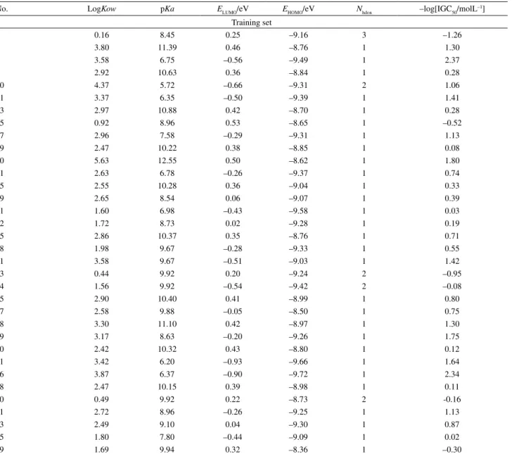
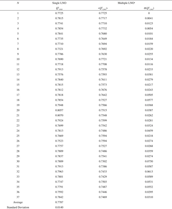
Among the validations performed for the real model (Table 2), the single LNO statistics shows an extraordinary behavior, with critical N = 37 (49% out), because the values
of Q2LNO stay high (Figure 1) and do not oscillate significantly
around the average value (Table T5) even at high N. Multiple
LNO shows slow but continuous decrease of average Q2LNO
and irregular increase of the respective standard deviations along N, so that up to N = 17 (23% out) two standard
deviations (±σ) are not greater than 0.1. (Table T5). In other words, the training set with 75 training toxicants is rather stable, robust to exclusion of large blocks (between 17 and 37 inhibitors), and the data split applied is effective.
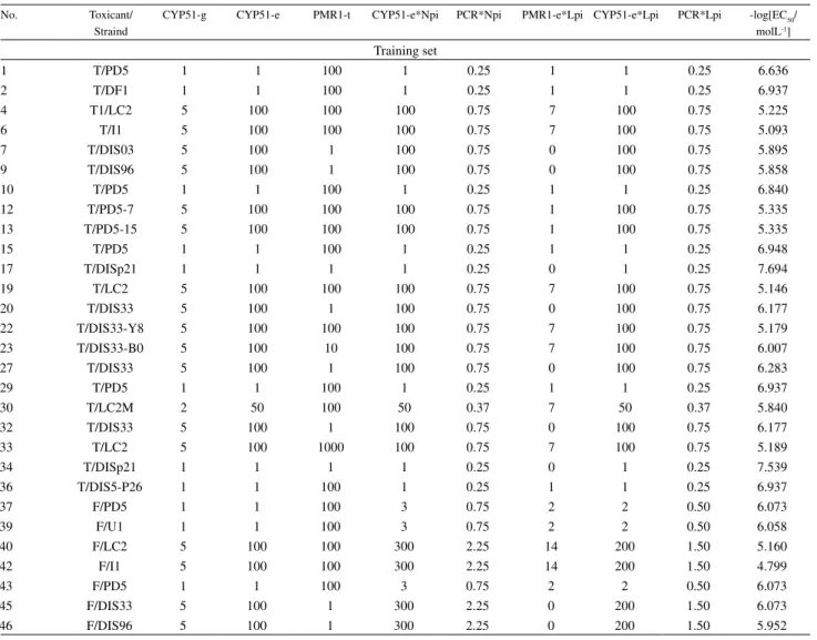
Three bootstrap schemes for 10 and 25 runs were applied (Tables T6 and T7) to form training sets: by random selection of 75 toxicants from the complete data set, from HCA clusters (10 clusters at the similarity index of 0.60), and from PCA groups (plot not shown). In fact,
Figure 1. Leave-N-out crossvalidation plot for the MLR model on data set 1. Black - single LNO, red - multiple LNO (10 times). Single LNO: average Q2 - dot-dash line, one standard deviation below and above the
average - dotted lines. Multiple LNO: one standard deviation below and above the average - red dotted curved lines.
Figure 2. A comparative plot for bootstrapping of the MLR model
three PCA groups were detected in the scores plot, based on three distinct values of descriptor Nhdon (see Table T1).
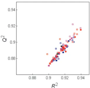
Classes of y were not applied since no gaps in the statistical distribution of y had been noticed. The graphical presentation of the results (Figure 2) shows that the data points are well concentrated along a R2 - Q2 diagonal, with
negligible dispersion in the region defined by R2 < 0.85
and Q2 < 0.80. The real model (the black point) is placed
in the middle of the bootstrap points. Careful comparison of the three bootstrap schemes indicates that HCA-based bootstrapping has certain advantages over the other two schemes. It is less dispersed and more symmetrically distributed around the real model. This would be expected, since each bootstrap training set originating from the HCA contains toxicants that represent well the complete data set in terms of molecular structure and descriptors.
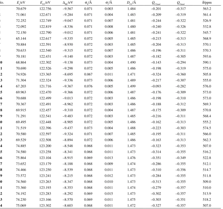
The real MLR model shows excellent performance in y-randomization with 10 and 25 runs (Tables T8 and T9). There are no randomized models in the proximity of the real model in the Q2 - R2 plot (Figure 3) since they are all
concentrated at Q2 < 0 and R2 < 0.2. A significantly larger
number of randomization runs should be applied to get some randomized models approaching the real model. This example illustrates how many randomized runs are necessary to detect a model free of chance correlation:
the choice of 10 or even 25 runs seems reasonable, which agrees with the method of Eriksson and Wold.53 When
the Q2 - r and R2 - r plots are analyzed (Figures F1 and
F2), it can be seen that the randomized models are placed around small values of r so that the intercepts of the linear
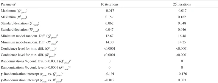
Table 3. Comparative statistics of 10 and 25 y-randomizations of the MLR model on data set 1
Parametera 10 iterations 25 iterations
Maximum (Q2
yrand) -0.017 -0.017
Maximum (R2
yrand) 0.157 0.182
Standard deviation (Q2
yrand) 0.062 0.048
Standard deviation (R2
yrand) 0.047 0.046
Minimum model-random. Diff. (Q2
yrand)b 12.67 16.48
Minimum model-random. Diff. (R2
yrand)b 14.30 14.25
Confidence level for min. diff. (Q2
yrand)c <0.0001 <0.0001
Confidence level for min. diff. (R2
yrand)c <0.0001 <0.0001
Randomizations %, conf. level > 0.0001 (Q2
yrand)d 0 0
Randomizations %, conf. level > 0.0001 (R2
yrand)d 0 0
y-Randomization intercept (ryrandvs.Q2
yrand)e –0.191 –0.176
y-Randomization intercept (ryrandvs.R2
yrand)e –0.012 0.003
aStatistical parameters are calculated for Q2 from y-randomization (Q2
yrand) and R2 from y-randomization (R2yrand).
bMinimum model-randomizations difference: the difference between the real model (Table 1) and the best y-randomization in terms of correlation coefficients
Q2
yrand or R2yrand, expressed in units of the standard deviations of Q2yrand or R2yrand, respectively. The best y-randomization is defined by the highest Q2rand or
R2 rand.
cConfidence level for normal distribution of the minimum difference between the real and randomized models. dPercentage of randomizations characterized by the difference between the real and randomized models (in terms of Q2
yrand or R2yrand) at confidence levels
> 0.0001.
eIntercepts obtained from two y-randomization plots for each regression model proposed. Q2
yrand or R2yrand is the vertical axis, whilst the horizontal axis is
the absolute value of the correlation coefficient ryrand between the original and randomized vectors y. The randomization plots are completed with the data
for the real model (ryrand = 1.000, Q2 or R2).
Figure 3. The y-randomization plot for the MLR model on data set 1:
regressions (1) and (2) are very small (aQ < –0.15 and aR ≤ 0.003, Table 3).
All the validations for the real MLR model confirm the self-consistency, robustness and good prediction power of the model, its stability to resamplings and the absence of chance correlation. The primary reason for this is the number of compounds. One out of five descriptors (the number of hydrogen bond donors, Nhdon, Table T1) shows
degeneracy, i.e., it has only three distinct integer values,
but it did not affect the model’s performance noticeably in this case.
Data set 2: QGSAR modeling of fungal resistance (P. digitatum) to demethylation inhibitors
Kiralj and Ferreira39 have used five latent variables
to model the complete data set of 86 samples using PLS (96.8% variance, Q2 = 0.851, R2 = 0.874, RMSECV =
0.286, RMSEC = 0.271, Q = 0.922 and R = 0.935), and also
for the data split with 56 training samples when building the auxiliary PLS model (97.1% variance, Q2 = 0.841, R2 = 0.881, RMSECV = 0.305, RMSEC = 0.279, Q = 0.917,
R = 0.939, Q2ext = 0.844, R2ext = 0.843, RMSEP = 0.272 and Rext = 0.935). The split (35% out) was done based on six
HCA clusters at a similarity index of 0.65. In this work, the model for 56 training samples was considered as the real model and it was further validated by bootstrapping. Results from validations for data set 2 are shown in Table 4 and in the Supplementary Information (Tables T10-T15 and Figures F3-F7).
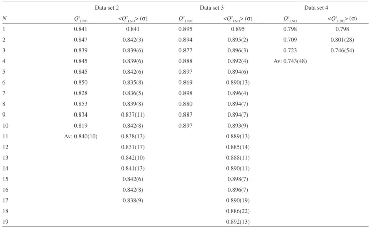
The single and multiple LNO statistics (Table 4, Table T10 and Figure F3) show that the critical N is 10
(leave-18%-out) and 17 (leave-30%-out), respectively. The variations of Q2
LNO in single LNO are uniform and less
than 0.1, and the same is valid for two standard deviations in multiple LNO. Therefore, the real model is robust to exclusion of blocks in the range of 10 - 17 samples, which is reasonable for a data set of this size.40
Four bootstrap schemes were applied (Tables T11 and T12) to randomly select 56 training samples from the following sets: 1) the complete data set; 2) the six HCA clusters; 3) three classes of y, based on its statistical distribution (low, moderate and high fungal activity referred to intervals 4.55-5.75, 5.76-6.75, and 6.76-7.70,
Table 4. Important resultsa of single (Q2
LNO)b and multiple (<Q2LNO> (σ))c leave-N-out crossvalidations for regression models on data sets 2, 3 and 4
Data set 2 Data set 3 Data set 4
N Q2
LNO <Q2LNO> (σ) Q2LNO <Q2LNO> (σ) Q2LNO <Q2LNO> (σ)
1 0.841 0.841 0.895 0.895 0.798 0.798
2 0.847 0.842(3) 0.894 0.895(2) 0.709 0.801(28)
3 0.839 0.839(6) 0.877 0.896(3) 0.723 0.746(54)
4 0.845 0.839(6) 0.888 0.892(4) Av: 0.743(48)
5 0.845 0.842(6) 0.897 0.894(6)
6 0.850 0.835(8) 0.869 0.890(13)
7 0.828 0.836(5) 0.898 0.896(4)
8 0.853 0.839(8) 0.880 0.894(7)
9 0.834 0.837(11) 0.887 0.894(7)
10 0.819 0.842(8) 0.897 0.893(9)
11 Av: 0.840(10) 0.838(13) 0.889(13)
12 0.831(17) 0.885(14)
13 0.842(10) 0.888(11)
14 0.841(13) 0.890(11)
15 0.842(6) 0.898(7)
16 0.842(8) 0.896(7)
17 0.838(9) 0.890(19)
18 0.886(22)
19 0.892(13)
aPartial results are shown for values of N at which Q2 is stable and high. bResults of single LNO: Q2
LNO - Q2 for a particular N, Av - average of Q2 with standard deviation in parenthesis (given for the last or last two digits). cResults of multiple LNO: <Q2
respectively); and 4) three MDR (multidrug resistance) classes of fungal strains with respect to pesticides (resistant, moderately resistant and susceptible).39 The graphical
presentation of the bootstrap models when compared to the real model (Figure F4), is very similar to that from data set 1. A new observation can be pointed out here, that the bootstrap models become more scattered as the number of runs increases, which is statistically expected. Resamplings based on HCA and y distribution seems to be the most adequate bootstrap schemes, because they are more compact and better distributed around the real model than those for the other two bootstrap schemes.
Results from 10 and 25 y-randomization runs (Tables T13 and T14) were analyzed numerically (Table T15) and graphically by means of the Q2 - R2 plot
(Figure F5), and Q2 - r and R2 - r plots (Figures F6 and F7).
The results are very similar to those from data set 1, leading to the same conclusion that the explained variance by the real PLS model is not due to chance correlation. In cases like this one, the results from a huge number of randomization runs18 would concentrate mainly in the region of these 10
or 25 randomizations, confirming the conclusions that the real PLS model is statistically reliable.
Data set 3: QSPR modeling of carbonyl oxygen chemical shift in substituted benzaldehydes
Kiralj and Ferreira5 have used two latent variables to
build the real PLS model for the complete data set of 50 benzaldehydes (92.3% variance, Q2 = 0.895, R2 = 0.915,
RMSECV = 9.10 ppm, RMSEC = 8.43 ppm, Q = 0.946
and R = 0.957), and also for the data split with 40 training
samples to construct an auxiliary PLS model (92.6% variance, Q2 = 0.842, R2 = 0.911, RMSECV = 9.59 ppm,
RMSEC = 8.83 ppm, Q = 0.942, R = 0.954, Q2ext = 0.937, R2
ext = 0.936, RMSEP = 6.79 ppm and Rext = 0.970). This
split (20% out) was done based on five HCA clusters with a similarity index of 0.70. In this work, these real and auxiliary models were further validated and the validation results were analyzed in detail.
The LNO statistics5 (Table 4, Table T16 and Figure F8)
show that Q2 stays high and stable up to the value of
N = 10 (leave-20%-out) in single LNO and N = 19
(leave-38%-out) in multiple LNO, after which it starts to decrease and oscillate significantly. This is a very satisfactory result for a modest data set of fifty samples.
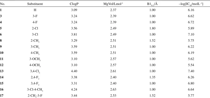
Three resampling schemes were applied in bootstrap validation (Tables T16 and T17) to exclude 10 from 50 samples randomly from the following sets: 1) the complete data set; 2) the five HCA clusters; and 3) three classes of y, based on statistical distribution of y (low, moderate and high chemical
shifts).5 Figure 4 shows the Q2 - R2 plot taking into account
all the resampling schemes for 10 and 25 runs. Unlike the analogues for data sets 1 and 2, a different type of dispersion of the bootstrap models is observed in the plot. In fact, the data points are not well distributed along a diagonal direction but are substantially scattered in the orthogonal direction, along the whole range of values of Q2 and R2. The auxiliary model (the
green point) is not in the centre of all bootstrap models, whilst the real model (the black point) is out of the main trend due to the different size of the training set. On the other hand, the plot still shows small variations in Q2 and R2, and no qualitative
changes in this scenario are expected when increasing the number of bootstrap runs. Differences with respect to the analogue plots from data sets 1 and 2 may be a cumulative effect of diverse factors, as for example, smaller training set size, different ranges and statistical distribution profile of y, and the nature of y (chemical shifts against negative logarithm of molar concentrations). The common point in the three data sets is the performance of HCA-bootstrapping over the other schemes.
Results from 10 and 25 y-randomization runs (Tables T18 and T19) were analyzed numerically (Table T20) and graphically (Figures F9 - F11). The Q2 - R2
plot (Figure F9) shows no chance correlation. It is likely that the results from a larger number of randomization runs would be concentrated in the region already defined. The
Q2 - r and R2 - r plots (Figures F10 and F11) also show the
absence of chance correlation, which is reconfirmed by numerical approaches in Table T20.
Figure 4. A comparative plot for bootstrapping of the PLS model on
The real model has somewhat weaker statistics than the previous one, but its statistics is still acceptable and in accordance to the data set size and recommendations for the five validation procedures.
Data set 4: QSAR modeling of mouse cyclooxigenase-2 inhibition by imidazoles
Hansch et al.55 have built a MLR model for this small
data set containing 15 inhibitors, with acceptable LOO statistics (reported: Q2 = 0.798, R2 = 0.886 and RMSEC =
0.212; calculated in this work: RMSECV = 0.241, Q = 0.895
and R = 0.941). Besides the real model, an auxiliary model
was constructed in this work, by considering inhibitors 4 and 10 (Table T4 in Supporting Information) as external validation samples. This data split, reasonable for such a small data set (13% out), was performed according to the HCA analysis which resulted in one large and one small cluster with 13 and 2 samples, respectively (dendrogram not shown). The two inhibitors selected were from the large cluster. The auxiliary model shows improved LOO statistics with respect to that of the real model (Q2 = 0.821,
R2 = 0.911, RMSECV = 0.239, RMSEC = 0.202, Q = 0.908
and R = 0.954). The external samples 4 and 10 are reasonably well predicted with calculated activities 6.52 and 6.49, respectively, compared to their experimental values 6.72 and 6.19, respectively, which means less than 5% error. The downside of this external validation is that it is not justified to calculate RMSEP, Q2ext or other statistical
parameters for a set of two inhibitors.
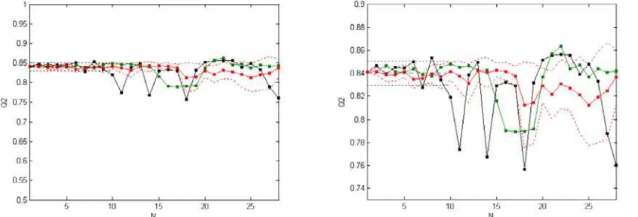
Both single and multiple LNO statistics (Table 4, Table T21 and Figure F12) show that the model is stable for
N = 1 - 3 (leave-20%-out). The values of Q2LNO in this interval
of N oscillate within the limit of 0.1 (see Figure F12). These
results indicate that the model is reasonably robust in spite of the data size.
The bootstrap tests for the MLR model were performed by eliminating two inhibitors by random selection from the complete data set and from the large HCA cluster. Other resampling schemes were not applied in this example due to the data size and its y distribution. The results obtained (Tables T22 and T23), when compared to that from the auxiliary model of the same data size (Figure 5), show rather unusual behavior. The data points in the R2 - Q2 plot
are not well distributed along some diagonal direction as in the analyses for data sets 1 and 2, but are rather dispersed in the orthogonal direction, especially at lower values of Q2
around 0.6. This suggests that Q2 would easily overcome
the limit of 0.65 with increasing the number of resamplings. The auxiliary model (the green point), which should be closer to the bootstrap models than the real model, is placed
too high with respect to the centroids of these models. The plot shows an unusual, “asymmetric” aspect unlike the analogue plots for data sets 1 - 3 (Figures 2 - 4), due to the pronounced differences between Q2 and R2 (see Tables
T22 and T23).
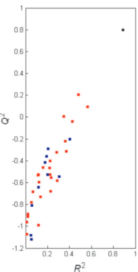
Results from 10 and 25 y-randomization runs (Tables T24 and T25), when presented graphically (Figure 6), show a large dispersion of the data points. The points are placed along a R2 - Q2 diagonal and also spread around
it. Furthermore, it is evident that a slight increase in the number of y-randomization runs would result in falsely good models that would be very close to the real model, meaning that this final model is based on chance correlation, and thus, is invalid. Compared to the previous y-randomization plots for data sets 1 - 3 (Figures 3, F5 and F9), a systematic increase of the dispersion of the data points can be observed. This trend is followed by the appearance of highly negative values of Q2 for the randomized models: about –0.2, –0.3,
–0.6 and –1.1 for data sets 1, 2, 3, and 4, respectively. To be more rigorous in this validation, further calculations were carried out, as shown in Table 5 and Figures F13 and F14. The smallest distance between the real model and randomized models is significant in terms of confidence levels of the normal distribution (<0.0001), both in Q2 and R2. The situation is even more critical when
all distances are expressed in terms of the confidence level, since more than 40% of the randomized models are not statistically distinguished from the real model in Q2
units, and much less but still noticeable in R2 units (for
more than 10 runs). These tendencies seem to be more
Figure 5. A comparative plot for bootstrapping of the MLR model on data
obvious when increasing the number of randomization runs. However, when the linear regression equations (1) and (2) are obtained, the intercepts do not approach the limits (aQ
< 0.05 and aR < 0.3) and the validation seems apparently
acceptable. It is obvious that this inspection is not sufficient by itself to detect chance correlation in the model and so, one has to investigate the spread of the data points in the region around the intercept in both Q2 - r and R2 - r plots. If
this spread is pronounced in the way that several data points are situated above the limits for intercepts, then the chance correlation is identified, which is exactly the situation in the present plots (Figures F13 and F14). In fact, the MLR model published by Hansch et al.60 has certainly failed in
y-randomization, confirming that small data sets seriously tend to incorporate chance correlation. The other possible reason, although of less impact, is data degeneration (redundancy) in columns and rows of the data matrix X (see Table T4 in Supporting Information). The cumulative results of y-randomization and the other validations show that the real MLR model is not statistically reliable.
Data quality versus data set size: data subset 3
The comparative discussion of models’ performance in previous sections was based on data set size. In this section,
Table 5. Comparative statistics of 10 and 25 y-randomizations of the MLR model on data set 4
Parametera 10 iterations 25 iterations
Maximum (Q2
yrand) –0.202 0.206
Maximum (R2
yrand) 0.404 0.563
Standard deviation (Q2
yrand) 0.316 0.341
Standard deviation (R2
yrand) 0.115 0.153
Minimum model-random. Diff. (Q2
yrand)b 3.16 1.74
Minimum model-random. Diff. (R2
yrand)b 4.19 2.10
Confidence level for min. diff. (Q2
yrand)c 0.0016 0.0819
Confidence level for min. diff. (R2
yrand)c <0.0001 0.0357
Randomizations %, conf. level > 0.0001 (Q2
yrand)d 40% 48%
Randomizations %, conf. level > 0.0001 (R2
yrand)d 0 24%
y-Randomization intercept (ryrandvs.Q2
yrand)e –0.989 –0.739
y-Randomization intercept (ryrandvs.R2
yrand)e –0.011 0.077
aStatistical parameters are calculated for Q2 from y-randomization (Q2
yrand) and R2 from y-randomization (R2yrand). Values typed bold represent obvious
critical cases.
bMinimum model-randomizations difference: the difference between the real model (Table 1) and the best y-randomization in terms of correlation coefficients
Q2
yrand or R2yrand, expressed in units of the standard deviations of Q2yrand or R2yrand, respectively. The best y-randomization is defined by the highest Q2rand or
R2 rand.
cConfidence level for normal distribution of the minimum difference between the real and randomized models. dPercentage of randomizations characterized by the difference between the real and randomized models (in terms of Q2
yrand or R2yrand) at confidence levels
> 0.0001.
eIntercepts obtained from two y-randomization plots for each regression model real. Q2
yrand or R2yrand is the vertical axis, whilst the horizontal axis is the
absolute value of the correlation coefficient ryrand between the original and randomized vectors y. The randomization plots are completed with the data for
the real model (ryrand = 1.000, Q2 or R2).
Figure 6. The y-randomization plot for the MLR model on data set 4: