The FORBIO Climate data set for climate analyses

(1)

www.adv-sci-res.net/12/103/2015/ doi:10.5194/asr-12-103-2015

The FORBIO Climate data set for climate analyses

C. Delvaux, M. Journée, and C. Bertrand

Royal Meteorological Institute of Belgium, Brussels, Belgium

Correspondence to:C. Delvaux (charles.delvaux@meteo.be)

Received: 13 January 2015 – Revised: 23 April 2015 – Accepted: 20 May 2015 – Published: 3 June 2015

Abstract. In the framework of the interdisciplinary FORBIO Climate research project, the Royal Meteorologi-cal Institute of Belgium is in charge of providing high resolution gridded past climate data (i.e. temperature and precipitation). This climate data set will be linked to the measurements on seedlings, saplings and mature trees to assess the effects of climate variation on tree performance. This paper explains how the gridded daily tem-perature (minimum and maximum) data set was generated from a consistent station network between 1980 and 2013. After station selection, data quality control procedures were developed and applied to the station records to ensure that only valid measurements will be involved in the gridding process. Thereafter, the set of unevenly distributed validated temperature data was interpolated on a 4 km×4 km regular grid over Belgium. The per-formance of different interpolation methods has been assessed. The method of kriging with external drift using correlation between temperature and altitude gave the most relevant results.

1 Introduction

The interdisciplinary FORBIO Climate research project wants to scrutinize the adaptive capacity of tree species and predict the future performance of tree species in Belgium under different scenarios of climate change. Towards this objective, the Royal Meteorological Institute of Belgium is in charge of providing high resolution gridded past climate data (i.e. temperature and precipitation) between 1980 and 2013. The gridded daily temperature (minimum and maxi-mum) data set was generated from the network of climato-logical stations administrated by the Royal Meteoroclimato-logical Institute of Belgium (RMI) since the end of the 19th century. In order to provide the high resolution gridded data set from the data of the station network, data quality control proce-dures were developed and the performance of different inter-polation methods has been assessed.

The RMI network relies on voluntary observers, profes-sional observers on civil and military aerodromes, federal agents, regional agents and employees of private companies. RMI supplies any voluntary observers with a manual rain gauge and a meteorological shelter in about 3/5 of the sta-tions. Air temperature is measured in a shaded enclosure (i.e., Stevenson screen) at a height of approximately 1.5 m above the ground. Maximum and minimum temperatures, for the

previous 24 h, are recorded at 08:00 LCT (local clock time). Minimum temperature is recorded against the day of the ob-servation, and the maximum temperature against the previ-ous day. Temperature records from both voluntary and syn-optic stations were considered to generate the 34-year-long (1980–2013) high resolution daily gridded temperature data set over Belgium. Within this period, 278 time series from the RMI database of climate observations contain at least one temperature record. However, a large number of time series contain missing observations. The total number of available observations per day varies between 109 and 175 over the considered time period (see Fig. 1, left panel). The spatial distribution of the corresponding stations within the Belgian territory is provided on the right panel in Fig. 1. Stations for which less than 5 % of the temperature records are missing over the considered time period are referred to as reference stations (i.e. 65 stations, see black dots in Fig. 1). The mean temperature over the 34 years obtained using the daily tem-perature observations from the 65 reference stations are pro-vided in Fig. 2 forTNandTX, respectively. Because no mea-suring technique is perfect and errors can run in meteorolog-ical observations for a wide variety of reasons (e.g. Aguilar et al., 2003), data were first quality controlled.

(2)

con-104 C. Delvaux et al.: The FORBIO Climate data set for climate analyses

Figure 1.Evolution of the number of available observations per day for the period 1980 to 2013 (left panel) and location of the stations in operation between 1980 and 2013 with the division into 4 climate zones (right panel). Reference stations (i.e. less than 5 % of missing temperature records) are indicated by a black dot while the other stations are represented by a yellow diamond.

3 4 5 6 7 8

10 11 12 13 14 15 16

Figure 2.Averaged temperature over the 34 years [◦C] forTN(left panel) andTX(right panels) using reference station records only. The interpolation was made using ordinary kriging method (see Sect. 3). The missing data are estimated by spatial interpolation.

trol (QC) procedures developed. Section 3 presents the considered interpolation methods. Results are presented in Sect. 4 and additional discussions are provided in Sect. 5. Final conclusions are given in Sect. 6.

2 Quality control procedures

2.1 Definition of quality control zones

For quality control purposes, geographical zones of similar temperature characteristics were defined based on the refer-ence stations temperature records. These zones will be used to compare stations of the same zone to each other and to de-fine quality control thresholds specific to each zone. The dif-ferent zones were identified byk-means clustering approach (Hair, 2009) based on mean and variability of the reference stationsTXandTNtime series.

A division into 4 zones was selected (see the right panel in Fig. 1). These zones broadly correspond to the Belgian coast (red), Flanders (green), Ardenne (purple) and the rest of Wallonia (blue).

2.2 Preliminary tests (time series evaluation)

In the first instance, two preliminary tests are applied on 1-year long time series to ensure the validity of the studied sta-tion. The first test (variability test) compares the data’s stan-dard deviationσ of the given station for a time period of one year to the expected limits. The minimum (maximum) limit corresponds to the half (double) of the reference sta-tions mean standard deviation. Ifσ lies outside the minimum and maximum thresholds, the entire time series is consid-ered as not usable. The second test (lag test) verifies that no one-day time lag is affecting the data. Each 1-year long tem-perature record with and without lag (forwards or backwards) were compared to neighboring stations. If the data fit is better with a lag, the entire time series is considered as not usable.

2.3 Daily data quality control

(3)

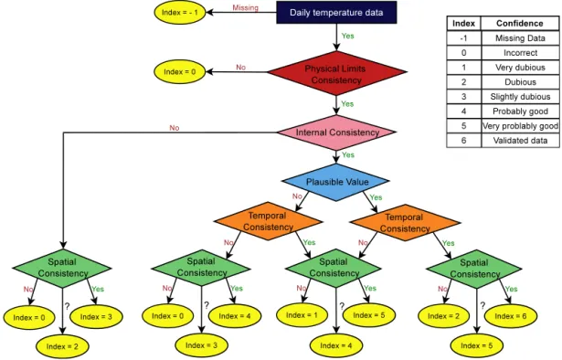
Figure 3.Automated QC applied to temperature records and associated confidence index.

temperature values for more subtle errors. Implementation of the automated QC is diagrammed in Fig. 3. Data are checked for internal consistency, plausible value test (using adapted limits to reflect climatic conditions more precisely than in the first range test), temporal consistency and spatial consis-tency. At the end of the process, a confidence index ranging from−1 to 6 (i.e. missing data to validated data) is attributed to each datum.

2.3.1 Physical limit consistency test

The aim of the physical limit consistency test is to ensure that temperature records stays within acceptable range limits using extreme climatological boundaries. These boundaries are based on the extreme values of the reference stations for each season and climate zone. To account for extreme values within the different zones, the boundaries are adjusted with a tolerance of 3◦C. Lower and upper limits for the four seasons are given for the Flanders and Ardenne zones in Table 1 for illustration.

2.3.2 Internal consistency test

The internal consistency test ensures that for a given dayTN

is not higher thanTX. Such an incoherence is technically pos-sible because TN is recorded one day later thanTX but is attached to the same day asTX.

Table 1. Extreme climatological boundaries for the Flan-ders/Ardenne zones per seasons used in the physical limit consis-tency test.

Lower limit Upper limit Lower limit Upper limit

TN[◦C] TN[◦C] TX[◦C] TX[◦C]

winter −26.5/−27.6 16.5/15.8 −15.2/−17.6 26.8/25.7

spring −12.8/−15.4 25.7/24 −2.8/−5.9 39.4/36

summer −1/−5.4 26/25.3 6.8/6 41.2/40

autumn −18.2/−23.2 21/18.2 −13.9/−14.2 31/29.9

2.3.3 Plausible value test

For the plausible value test, dailyTNandTXvalues are com-pared to daily lower and upper bounds. For each of the 4 cli-mate zones, lower and upper bounds for a given temperature data series (i.e.TNandTX) are constructed by retrieving the highest and lowest daily values on each calendar daydof the year from 34 years of data. Assuming that the annual temper-ature variations follow a sinusoidal wave, a fit of the annual variation of these extreme temperatures is defined using wave functionTL/U(d). An observation succeeds the test if it stays within the lower and upper bounds of the corresponding day (Sciuto et al., 2013).

2.3.4 Temporal consistency test

(4)

pre-106 C. Delvaux et al.: The FORBIO Climate data set for climate analyses

Table 2.Percentage of the different indexes obtained after the QC procedures. Note that to maintain a good comparison between both types of stations, the “missing data” are not included in the index percentage of index 0 to 6.

Index percentage

Index Reference Other stations stations

[%] [%]

−1 3.32 61.22

0 0.001 0.002 1 0.003 0.005 2 0.008 0.008 3 0.029 0.036 4 0.008 0.014 5 0.593 0.640 6 99.358 99.301

ceding acceptable level. The maximum probable change is based on the 99th percentile change for the 34 years of data. The test is applied by season and climate zone with a one-day time step. Similarly a persistence test (1min) flags the measurements that fail to change by more than a minimum amount.

2.3.5 Spatial consistency test

The spatial consistency test compares the observations at a given station with the observations of the same day made at neighboring stations. The result is suspicious (represented by a question mark in Fig. 3) if the station record differs for more than 2.5◦_{C from each of its 3 closest neighboring} stations or by more than 4◦_{C of the averaged values of the} 3 closest neighboring stations. The observation fails the spa-tial consistency tests if the two values above become respec-tively 5 and 7◦C (these values are based on the expertise of the well qualified RMI’s data quality agents). A nearby sta-tion is considered only if the difference in elevasta-tion with the studied station is below 150 m.

2.4 Confidence Index

More than 5 millions of temperature records (TN andTX) were faced to the data quality control protocol described above. More than 99.3 % of the analyzed records have suc-ceeded the different tests (confidence index of 6). The pro-portion of data classified as at least “very probably good” (confidence index greater than 5) was of 99.95 %. Table 2 compares the results in terms of attributed confidence index obtained at the reference stations and at the other stations.

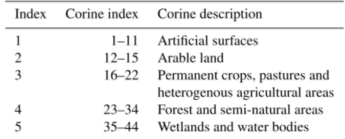
Table 3.Correspondance between Corine Land Cover database and the five land cover types used in this study.

Index Corine index Corine description

1 1–11 Artificial surfaces 2 12–15 Arable land

3 16–22 Permanent crops, pastures and heterogenous agricultural areas 4 23–34 Forest and semi-natural areas 5 35–44 Wetlands and water bodies

3 Interpolation methods

Long-term climate patterns observed across the globe are a result of a combination of many different processes that man-ifest themselves at many spatial scales. It is assumed that most of those patterns occur at scales large enough to be ad-equately reflected in the station data, and thus are not explic-itly accounted for by the major interpolation methods. The main physiographic features affecting spatial patterns of cli-mate are terrain and water bodies (e.g., Daly, 2006). Several additional spatial climate foreigns factors are most important at scales of less than 1 km but may also have effects at larger scales. These factors include slope and aspect, riparian zones and land use/land cover (Lookingbill and Urban, 2003; Mc-Cutchan and Fox, 1986; Bolstad et al., 1998; Dong et al., 1998).

For each day of the considered 34-year-long time period (i.e. 1 January 1980 to 31 December 2013), all the validated (i.e. confidence index of 6) stations temperature records (i.e.TNandTX) were interpolated on a regular 4 km×4 km grid over Belgium. To predict the unknown values from the unevenly distributed temperature records observed at known locations, the performance of different interpolation meth-ods has been assessed: inverse distance weighting (IDW), or-dinary kriging (OK) and kriging with external drift (KED; Wackernagel, 1995) that is able to handle densely sampled auxiliary variables highly correlated with the parameter of interest. In this study, KED was used with either the orogra-phy (KED1) or land cover types (KED2) as a drift, as well as

simultaneously with the two drifts (KED12). For the kriging

methods, the parameters used to estimate the semivariogram were fixed in order to have an exact interpolation at the sta-tion locasta-tion (i.e. the estimasta-tion satisfies the observasta-tion at the station location) with a fixed range of 50 km and an ex-ponential semivariogram model.

(5)

0 100 200 300 400 500 600 700 1 2 3 4 5

Figure 4.4 km resolution orography of Belgium [m] (left panel) and 4 km resolution CORINE Land Cover in Belgium (right panel).

● ● ● ● ● ● ●● ● ● ● ● ● ● ● ● ● ● ● ● ● ● ● ● ● ● ● ● ● ● ● ● ● ● ● ● ● ● ● ● ● ● ● ● ● ● ● ● ● ● ● ● ● ● ● ● ● ● ●

0 100 200 300 400 500 600 700

3 4 5 6 7 8 Mean TN Altitude [m] T emper ature [°C] ●● ● ● ● ● ● ●●● ●● ● ● ●● ● ● ● ●● ● ● ● ● ● ● ● ● ● ● ● ● ● ● ● ● ● ● ● ● ● ● ● ● ● ● ● ● ● ● ● ● ● ● ● ● ● ●

0 100 200 300 400 500 600 700

10 12 14 16 Mean TX Altitude [m] T emper ature [°C]

Figure 5. Correlation between station elevation and daily mean temperature (for the reference stations). The correlation coefficients are of−0.85 and−0.93 forTNandTX, respectively.

dominant land cover class within a given grid point is at-tributed to the entire grid point).

The various interpolation approaches are validated by leave-one-out cross-validation. For each day of the con-sidered period, the cross-validation root mean square error (RMSEcv) is computed from the differences between the

pre-dictionP and the actual measurementsMat thenstations:

RMSEcv=

s 1 n n P i=1

(P(xi)−M(xi))2 where {xi}i=1,...,n is

the location of the climate stations.

To determine the best performing method, two indices are derived from the daily RMSEcv. First, the averaged over the

34 years (i.e. RMSEAVG_cv ) and second, the frequency of the method providing the best daily RMSEcv over the 34 years

(i.e. RMSEFREQcv ).

4 Results

Table 4 summarizes the performance of the investigated in-terpolation methods in terms of RMSEAVG_cv and RMSEFREQcv

index for bothTNandTX, respectively. Results indicate that for TN all methods perform quite similarly: the averaged accuracy (RMSEAVGcv ) ranges from 0.867 for the “worst”

method (IDW) to 0.818 for the best one (KED1). By

con-trast the interpolatedTXfields appear more sensitive to the considered methods. As forTN, the best performing method is KED1and the worst one is IDW but the magnitude of the

difference between the two methods in terms of RMSEAVGcv

is larger (i.e. 0.14◦C vs. 0.05◦C forTN). This difference be-tweenTNandTXcan be explained by the larger correlation found over our domain between the elevation andTXthan for

TN(see Fig. 5).

Accounting for the land cover type in the interpolation scheme does not improve the results for bothTN and TX. The difference in terms of RMSEAVG_cv between OK and KED2

is clearly negligible (i.e. 0.852◦C vs. 0.854◦C forTN and 0.721◦C vs. 0.723◦C forTX). Similarly using the land cover type in addition to the orography in the kriging with ex-ternal drift approach does not significantly modify the per-formance obtained when only considering the orography as drift (e.g. RMSEAVGcv of 0.818◦C for KED1vs. 0.820◦C for

KED12in the case ofTNand 0.601◦C for KED1vs. 0.605◦C

for KED12 in the case of TX, respectively). This is not so

surprising in view of the spatial resolution adopted for the gridding (e.g. 4 km×4 km) as the land use/land cover varia-tions are expected to be most important below 1 km. Analysis of the RMSEFREQcv provided in Table 4 confirm that the best

performing interpolation method in terms of RMSEcvis the

kriging using the orography as external drift (KED1) for both

TNandTX(e.g. RMSEFREQcv of 43 % forTNand RMSEFREQcv

of 77.1 % forTX). What is interesting to note regarding the RMSEFREQcv in Table 4 is the score obtained by the kriging

using the land cover type as external drift (KED2). Indeed,

for bothTNandTX, the value of this index for the KED2is

(6)

108 C. Delvaux et al.: The FORBIO Climate data set for climate analyses

Table 4.Overall performance of the different interpolation methods over the entire time period expressed in terms of RMSEAVG_cv and RMSEFREQ_cv for bothTXandTN.

RMSEAVG_cv RMSEAVG_cv RMSEFREQcv RMSEFREQcv

(TN)[◦C] (TX)[◦C] (TN)[%] (TX)[%]

IDW 0.867 0.738 14.5 0.6

OK 0.852 0.721 15.1 1.1

KED₁ 0.818 0.601 43 77.1

KED₂ 0.854 0.723 7.9 0.3

KED₁₂ 0.820 0.605 19.5 20.9

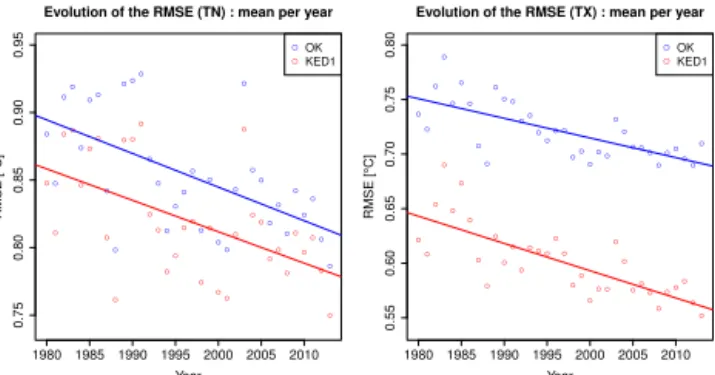
Finally, Fig. 6 displays the time evolution of the annual mean daily RMSEcv over the considered 34-year-long time

period obtained by using the OK and the KED1daily

inter-polation methods, respectively. Both methods present a clear reduction of the RMSEcv throughout the time forTX with

the largest reduction obtained by the KED1 approach (see

left panel in Fig. 6). Similar behavior is also observed forTN

while for this parameter the dispersion is a bit more larger than forTX(see right panel in Fig. 6). The reduction of the annual mean daily RMSEcvhas to be put in connection with

the increasing number of stations involved in the interpola-tion process with time (see Fig. 1, left panel).

5 Discussion

As an additional validation exercise, the newly developed FORBIO climate data set was compared to existing data sets. Towards this objective, the RMSE results presented in Sect. 4 are compared to these obtained from the HYRAS data set which cover Germany (Frick et al., 2014). This data set has a similar resolution (5 km) and use the Optimal Interpola-tion method. The fivefold cross-validaInterpola-tion of HYRAS gives an averaged RMSE of 1.39◦C versus values from 0.601◦C to 0.867◦C for the FORBIO climate data set. The better sta-tion density and the smaller elevasta-tion differences between stations can explain the better results obtained in the FOR-BIO data set.

The new FORBIO data set can also be compared to the ex-isting E-OBS data set (version 10.0) (Haylock et al., 2008), which provides daily temperature data for the period 1950– 2013 on a regular 0.25◦grid (approximately 25 km). 16 Bel-gian synoptic stations are used in the E-OBS data set. To al-low a comparison at the same resolution, the FORBIO data set was first degraded at the E-OBS resolution. Figure 7 shows the differences between the two data sets using the mean maximum temperature over the 34 years. The benefit of the original FORBIO data set spatial resolution is evident for the user. At the degraded resolution, a major difference between the two data sets (>1◦C) appears in the Hainaut Province. Only one station located in the Hainaut Province is considered with the E-OBS data set (i.e. the Chièvre syn-optic station, black dot in Fig. 7) and this station appears

● ● ● ● ● ●● ● ● ●●● ● ● ● ● ● ● ● ● ● ● ● ● ● ● ● ● ● ● ● ● ● ●

1980 1985 1990 1995 2000 2005 2010

0.75

0.80

0.85

0.90

0.95

Evolution of the RMSE (TN) : mean per year

Year RMSE [°C] ● ● ●● ● ● ● ● ● ● ● ● ● ● ● ● ●● ● ● ● ● ● ● ● ● ● ● ● ● ● ● ● ● ● ● OK KED1 ● ● ● ● ● ● ● ● ● ● ● ● ●● ● ● ● ● ●● ● ●● ● ● ● ● ● ● ●● ● ● ●

1980 1985 1990 1995 2000 2005 2010

0.55 0.60 0.65 0.70 0.75 0.80

Evolution of the RMSE (TX) : mean per year

Year RMSE [°C] ● ● ● ● ● ● ● ● ● ● ● ● ● ● ● ● ● ● ● ● ● ● ● ● ● ●●● ● ●●● ● ● ● ● OK KED1

Figure 6.Evolution of the averaged annual RMSEcvand regression

line using ordinary kriging (OK) and kriging with external drift us-ing orography (KED1) forTN(left panel) andTX(right panel).

too cold compared to the neighboring climatological stations used in the FORBIO data set in addition to the Chièvre sta-tion records. This comparison is also true for minimum tem-perature.

6 Conclusions

To meet the needs of the FORBIO Climate research project, a 34-year-long (1980–2014) daily gridded temperature (min-imum and max(min-imum) has been produced over Belgium at a 4 km×4 km spatial resolution. Because no measuring tech-nique is perfect and errors can run in meteorological observa-tions for a wide variety of reasons, data quality control pro-cedures were developed and applied to temperature records performed within the Belgian climatological station network operated by RMI prior to undergo the daily gridding pro-cess. More than 5 millions of daily temperature records (TN

andTX) were analyzed in depth and about 0.7 % of these were discarded. The performance of 5 different interpola-tion methods was assessed over the Belgian domain ranging from the simple inverse-distance weighting approach to the kriging with external drift methods. Two auxiliary drifts have been considered (i.e. the orography and the land cover type) either individually or in combination. Because of the spatial resolution of 4 km×4 km adopted for the data set, it has been found that accounting for the land cover type in the interpo-lation process of temperature over Belgium is not relevant. By contrast using the orography as external drift in the krig-ing interpolation scheme provides the best results in term of RMSEcvand RMSEFREQcv for bothTXandTN. It is however

(7)

●

11 12 13 14 15

●

11 12 13 14 15

●

11 12 13 14 15

●

−1.0 −0.5 0.0 0.5 1.0

Figure 7.Averaged value forTXover the 34 years [◦C]: FORBIO (4 km resolution), FORBIO (25 km resolution), E-OBS (25 km resolution), differences between FORBIO and E-OBS. The black dot corresponds to the Chièvre station.

the Hainaut province where the E-OBS data set is colder. A minimum of 80 stations per day were always used in the grid-ding process for bothTNandTX. Note that in average over the 34 years a bit more stations were involved in the spatial interpolation ofTXthan forTN(i.e. 137 vs. 132 stations, re-spectively). Finally, because the number of stations involved in the daily gridding process has increased with time (even if the total number of available stations has started to decrease in the last decade covered by the dataset), the daily RMSEcv

present a clear reduction as a function of time for bothTX

andTN. As an example, the annual mean daily RMSEcvhas

decreased by 0.085◦C from 1980 to 2013 for TX and by 0.068◦C forTN.

Acknowledgements. This work was supported by the Belgian Science Policy Office (BELSPO) through the BRAIN-be program contract NR BR|132|A1|FORBIO CLIMATE “Adaptation potential of biodiverse forests in the face of climate change”. We acknowl-edge the E-OBS dataset from the EU-FP6 project ENSEMBLES (http://ensembles-eu.metoffice.com) and the data providers in the ECA & D project (http://www.ecad.eu). The “gstat” Package (version 1.0-22) in R (Pebesma, 2004) was used for geostatistical interpolation.

Edited by: I. Auer

Reviewed by: three anonymous referees

References

Aguilar, E., Auer, I., Brunet, M., Peterson, T., and Wieringa, J.: Guidelines on climate metadata and homogenization, World Cli-mate Programme Data and Monitoring WCDMP-No. 53, WMO-TD No. 1186, World Meteorological Organization, Geneva, 2003.

Bolstad, P. V., Swift, L., Collins, F., and Régnière, J.: Measured and predicted air temperatures at basin to regional scales in the south-ern Appalachian mountains, Agr. Forest Meteorol., 91, 161–176, 1998.

Bossard, M. and Feranec, J.: Otahel, Jaffrain, Gabriel, CORINE Land Cover technical guide – Addendum 2000, Tech. rep., Tech-nical Report 40, EEA, Copenhagen, http://www.eea.eu.int (last access: 8 January 2015), 2000.

Boulanger, J.-P., Aizpuru, J., Leggieri, L., and Marino, M.: A pro-cedure for automated quality control and homogenization of his-torical daily temperature and precipitation data (APACH): part 1: quality control and application to the Argentine weather service stations, Climatic Change, 98, 471–491, 2010.

Daly, C.: Guidelines for assessing the suitability of spatial climate data sets, Int. J. Climatol., 26, 707–721, 2006.

Dong, J., Chen, J., Brosofske, K., and Naiman, R.: Modelling air temperature gradients across managed small streams in western Washington, J. Environ. Manage., 53, 309–321, 1998.

Feng, S., Hu, Q., and Qian, W.: Quality control of daily meteorolog-ical data in China, 1951–2000: a new dataset, Int. J. Climatol., 24, 853–870, 2004.

Frick, C., Steiner, H., Mazurkiewicz, A., Riediger, U., Rauthe, M., Reich, T., and Gratzki, A.: Central European high-resolution gridded daily data sets (HYRAS): Mean temperature and rela-tive humidity, Meteorol. Z., 23, 15–32, 2014.

Hair, J. F.: Multivariate data analysis, Prentice Hall, Upper Saddle River, 2009.

Haylock, M., Hofstra, N., Klein Tank, A., Klok, E., Jones, P., and New, M.: A European daily high-resolution gridded data set of surface temperature and precipitation for 1950–2006, J. Geo-phys. Res.-Atmos., 113, D20119, doi:10.1029/2008JD10201, 2008.

Lookingbill, T. R. and Urban, D. L.: Spatial estimation of air tem-perature differences for landscape-scale studies in montane envi-ronments, Agr. Forest Meteorol., 114, 141–151, 2003.

McCutchan, M. H. and Fox, D. G.: Effect of elevation and aspect on wind, temperature and humidity, J. Clim. Appl. Meteorol., 25, 1996–2013, 1986.

Pebesma, E. J.: Multivariable geostatistics in S: the gstat package, Comput. Geosci., 30, 683–691, 2004.

Sciuto, G., Bonaccorso, B., Cancelliere, A., and Rossi, G.: Proba-bilistic quality control of daily temperature data, Int. J. Climatol., 33, 1211–1227, 2013.