*e-mail: [email protected]
Received: 26 February 2013 / Accepted: 05 November 2013
A maximum margin-based kernel width estimator and its application
to the response to neoadjuvant chemotherapy
Maria Fernanda Barbosa Wanderley*, Luiz Carlos Bambirra Torres, René Natowicz, Antônio Pádua Braga
Abstract Introduction: Function induction problems are frequently represented by afinity measures between the elements of the inductive sample set, and kernel matrices are a well-known example of afinity measures. Methods: The objective of the present work is to obtain information about the relations between data from a calculated kernel matrix by initially assuming that those geometric relations are consistent with known labels. To assess the relation between the data structure and the labels, a classiier based on kernel density estimation (KDE) was used. The performance of the selected width using the method presented in this paper was compared to the performance of a method described in the literature; the literature method was based on minimizing error minimization and balancing bias and variance. The main case study, which was to predict the response to neoadjuvant chemotherapy treatment, consists of evaluating whether a set of training data from genomic expression data from breast tumors and the genomic expression from the tumor of one patient can be used to determine whether there will be a pathological complete response. Results: For the tested databases, the proposed method showed statistically equivalent results with the literature method; however, in some cases, the proposed method had a better overall performance when considering both large and small classes. Conclusion: The results demonstrate the feasibility of selecting models by directly calculating densities and the geometry from the class separation.
Keywords Kernel, Classiication model, Maximum margin, Neoadjuvant chemotherapy.
Introduction
Induction of function problems are frequently represented by afinity measurements, or distance metrics, between the elements of the set of inductive samples. Inductive approximations are based on the relative similarity measures between the training samples and their labels. The use of kernel matrices to represent afinities became widespread after the popularization of support vector machines (SVMs) (Vapnik, 1999), where kernels are used to represent the inductive sample set in the feature space (Cortes and Vapnik, 1995; Vapnik, 1999) through non-linear mappings. The kernel matrix, where the non-linear transformation is performed, also contains the similarity measures between the samples and groups of samples for all the elements of the inductive set.
Non-parametric kernel density estimation (KDE) uses those matrices to deduce a function from the structural information contained in data; this method only uses the kernel function width as a parameter and does not require a priori assumptions about the
generating function.
In this work, we propose a method to estimate the kernel width based on the concept that the separation region between classes must occur at a low density location (Chapelle et al., 2006), thus minimizing the
model error. Simultaneously, we aim to control the complexity of the model, characterizing the problem as bi-objective.
The proposed method does not aim to construct a universal classiication model; instead, the method aims to explore the possibility of deducing functions from the geometric information in data that are obtained from the kernel function. We show that the results are comparable to those obtained from a method that assumes that the data were generated from a Gaussian function and attempts to balance the bias and variance of the model; this inding conirms the hypothesis of consistency between assigned labels and the function that generated the data.
Methods
Given a set Du = {xi}N
i=1, where N is the sample size,
the elements aij form an afinity matrix A = [aij] that
contains a measure of the afinity (or similarity) between the samples (xi, xj) (Scott and
Longuet-Higgins, 1990). Similarities measures are usually relexive; thus, the matrix A is generally symmetric, that is, aij = aji. There are many ways to represent
clustering methods (Johnson, 1967), and kernels. The Gaussian kernel is represented in Equation 1, as follows
2
i j
x x h i j k(x , x )= e
−
−
(1)
where h is the radius or standard deviation of the
Gaussian function, and k(xi, xj) = aij.
For a given value of h, the N×N kernel matrix
that results from Equation 1 contains the relexive relationships for all pairs (xi, xj) and can be represented as a diagonal block matrix, as shown in Equation 2,
11 12 1c
21 22 2c
c1 c2 cc
K = K K K
K K K
K K K
…
…
…
…
(2)
where c is the number of clusters from the sample
set Du = {xi}N i=1.
Each of the sub-matrices Kij from Equation 2 contains the afinity measures between the elements of groups i and j from the sample set. Therefore, the
representation as clusters also allows other important information to be extracted from the kernel matrix, such as information about the data distribution and the relationship between the samples and sample sets. In Figure 1, 150 bidimensional vectors are presented; these vectors were sampled from 5 Gaussian distributions with means m1 = [1, 4], m2 = [3, 4],
m3 = [4, 4], m4 = [2, 2], and m5 = [4, 2] and standard deviation 0.3. Figure 2 represents the Gaussian kernel matrix that results from the samples of Figure 1; the samples were ordered according to the generating distributions, which were known beforehand for this example. Figure 2 shows that the afinity relationship between elements from the same group and from different ones is visually distinguishable in this type
of representation, demonstrating the power of the information contained inside the kernel matrix.
The representation of afinities as a kernel matrix allows classiication and regression models to be deduced from data (Cortes and Vapnik, 1995). Furthermore, the matrix contains the information for deducing an estimator for f (x), the generating density
function of the set Du = {xi}N i=1.
Kernel density estimators, which will be described in the next sub-section, utilize relexive relationships
k(xi, xj) = kij to make local estimations of the density
function f (x), the function that generates the data.
Those non-parametric estimators only have one adjustable parameter; this parameter is usually related to the kernel smoothness, for example, the h parameter of Equation 1. Although kernel density estimators only rely on one global parameter, neither the number of variables nor the approximating multimodal density functions are limited. Thus, kernel density estimators are potentially attractive for applications where the samples and a priori information about the density
function that generated the data are scarce; these two situations frequently occur in bioinformatics problems.
Kernel Density Estimator – KDE
A kernel density estimator, or KDE (Parzen, 1962), is obtained by the superposition of kernel functions, as described in Equation 1, that are centered on each of the elements xi(i = 1...N) from the sample set.
The density estimator ^f (x
t) at xt depends only on the spatial relationship between xt and the elements of
the sample xi(i = 1...N); this relationship is quantiied
by the metric embedded in the kernel function. In general, Equation 3 describes a univariate kernel density estimator.
Figure 1. Bidimensional data sampled from ive distinct distributions
with means m1 = [1, 4], m2 = [3, 4], m3 = [4, 4], m4 = [2, 2], and
m5 = [4, 2] and standard deviation 0.3.
1 ˆ
t t i
f(x )= K(x , x )
Nh∑ (3)
In Equation 3, N is the sample size, h is the kernel
smoothing parameter, and K(xt, xi) is the kernel
operator, whose integral ∫K(u)du must be unitary. The
argument of the function K(.) is, in fact, the point xt
where one wants to make the estimation, given that the samples xi(i = 1...N) are ixed and known beforehand.
An example of an estimation with a KDE is shown in Figure 3. This igure shows a histogram representation and the continuous estimation of Equation 3 for data sampled from two normal distributions with means at –4 and 4. The KDE estimation represents the joint distribution of two modes of the generating function. Utilizing the parametric model of this bimodal distribution requires inding the two generating partitions, modeling each of them individually and then mixing them to obtain the joint distribution. In addition, the clustering parameters, such as the number of partitions, and the parameters of each individual distribution must be estimated. The estimation with KDE only requires determining the parameter h, which is associated with the spread of the Gaussian function.
Multidimensional KDE
If the input variables are independent, a multivariate density estimation with KDE, as described by Equation 3, can be obtained directly through multidimensional kernel functions, which are described in Equation 1. However, in the case of dependency, the KDE estimation also considers using different values of h for each of the dimensions of the vector x.
Consider that an arbitrary vector xj can be represented with its n dimensions as xj = (xj1, xj2, ..., xjn). Consequently, the general form of the multidimensional KDE is presented in Equation 4.
( )
(
)
1
1 2 1
1
ˆ N t1 i1 tn in
t
i=
n n
x x x x
f x = K , ,
N h h h h h
− … −
∑
∗ ∗…∗ (4)
An alternative to a multidimensional kernel function is the multiplicative kernel (Scott, 1992). In this case, a unidimensional kernel is used for each of the dimensions, and each kernel has its own width
h. Thus, the n-dimensional kernel is represented by
the product of kernels in each of the n univariate dimensions, resulting in Equation 5.
( )
1 1
1 1
ˆ N n j ij
h
j=
i= j j
x x
f x = K
N h h
−
∑ ∏
(5)
Assuming independence and the same width h for all dimensions, the Gaussian KDE density estimation of a given arbitrary point xi may be obtained through the
sum of the cumulative products in all dimensions for
all variables of the sample set. Re-writing the product and considering that the summation of Equation 5 corresponds to the sum of all elements of a line (or column) of the Gaussian kernel matrix K(xi, xk) = [kij] with width h, Equation 6 is obtained.
( )
(
)
1
1
ˆ N
h i n i k
k= f x = K x , x
Nh ∑ (6)
At this point, it is important to stress that the Gaussian kernel for density estimation using the multiplicative method and the one used for building inductive models, such as SVMs, have the same shape and only differ by the parameter h. Thus, the same
parameter h might be able to satisfy both problems
(Queiroz et al., 2009) when the density is estimated by KDE using a multiplicative kernel.
According to Equation 6, the density estimation ^
fh(xi) decreases upon locating the h value that
satisies some restriction of the objective function. However, determining the characteristics of the objectives that are used to estimate density functions is not as straightforward once the problem becomes unsupervised. Previously, Silverman (1986) described a method for estimating h by assuming that the generative
functions are Gaussians. Aiming to approximate the Gaussian function that generated the data and to balance the bias and variance (Geman et al., 1992) of the model, the author deined an objective function to determine h.
In contrast to Silverman’s (1986) approach, in this work, data normality is not assumed when determining
h through an objective function. The basic principle of
the approach presented in the following sub-sections is that structural information of the data, which are contained in the sample set D = {xi, yi}N
i=1, is suficient
to determine h. This principle seems to be valid,
particularly given that the same kernel can represent Figure 3. Density estimation performed with a histogram and with
the data structure and serve as a basic element for deducing models such as SVMs, as stated in previous paragraphs. The challenge of this approach, however, is to obtain coherent structural information using only the sample set and to describe this information using a quantitative measure that can be used to determine
h.The method that will be presented is based on the idea that the solution to the classiication model should be located in a low density region; this principle is one of the assumptions of semi-supervised learning (Chapelle et al., 2006). The model is smoothed by adjusting h based on the consistency of the responses
to the kernel function at the separation region, and this smoothing allows for control of the bias and variance and the separation margin between classes (Vapnik, 1999; Geman et al., 1992).
Selection method
Constructing generative classiiers by estimating the density of the generative functions relies on coherence between the labels that are given to data and the functions that have generated the data. Thus, according to this principle, the estimated generative functions, i.e., KDE, should be consistent with the labels yi given a sample set D = {xi, yi}N
i=1. For
Bayesian classiiers, the a posteriori probability
P(Cj | xi)that a pattern belongs to a given class Cj
should be greater for the class to which the pattern has been assigned. This principle not only guarantees the minimization of the empiric risk (Vapnik, 1999) of the data set but also guarantees the robustness of the model before its application to the test set. For binary classiication problems with two classes, C1
and C2, the ratio between the posterior probabilities
determines the classiier represented in Equation 7.
( )
(
(
1)
)
21
2
2
P x C N Class x = C ,if >
P x C N1
C ,otherwise.
(7)
Based on labeling information, the likelihoods
P(x | C1) and P(x | C2) for the classes C1 and C2, respectively, can be estimated with KDE, and a inal classiication can be performed. As discussed in the previous sub-sections, a consistent estimation of the densities by KDE will depend on the chosen value of h for Gaussian kernels. Nevertheless, knowing the
labels yi allows for analysis of the problem based on
the coherence between the generative density function and the labels given to each sample.Consider the sample set shown in Figure 4 and its matrix K for
h = 1, as presented in Figure 5. Although this example
is synthetic and well controlled, it represents the problem in a general way.
Visualizing the kernel matrix that corresponds to the data clearly allows for the identiication of four
distinct sub-matrices that form the kernel, which will be termed K11, K12, K21 and K22. Those two
data groupings represent two distinct classes: the sub-matrices K11 and K22 contain the intra-class
relationships, and the sub-matrices K12 and K21
contain the interclass relationships. Thus, the density estimation according to Equation 6 can be re-written by determining the estimated densities for the adjacent matrices, as in Equations 8 and 9. In these equations, the terms P({xi, yi = –1} | C1), P({xi, yi = –1} | C2),
P({xi, yi = +1} | C1) e P({xi, yi = +1} | C2) represent the P(xi | Ci) estimated for the labels yi.
{ }
( 1) ( )1 ({ } 2) ( )2
1 2
, 1 | , 1 |
1 11 12
1 1
1 1
ˆ ( ) ( , ) ( , )
i i i i
P x y C P C P x y C P C
N N
i n i k n i p
k p
f x C K x x K x x
Nh Nh
= − = −
= =
∈ = ∑ + ∑
(8)
{ }
( 1) ( )1 ({ } 2) ( )2
1 2
, 1 | , 1 |
2 21 22
1 1
1 1
ˆ ( ) ( , ) ( , )
i i i i
P x y C P C P x y C P C
N N
i n i k n i p
k p
f x C K x x K x x
Nh Nh
= =
= =
∈ = ∑ + ∑
(9) Figure 4. Data sampled from two Gaussian distributions with means m1 = [2, 2]T and m
2 = [4, 4] T.
P(C1) and P(C2) are known; therefore, it is possible
to estimate the likelihood of the patterns for each of the classes, C1 and C2, using Equations 10 through 13.
For a binary classiication problem, the probabilities estimated by Equations 10 and 12 are expected to be maximized and those estimated by Equation 11 and 13 are expected to be minimized for each pattern
xi∈D. Indeed, maximizing the difference between
those two quantities provides a method of minimizing the approximation error of the data set using only the coherence of the labeling and the estimated densities.
{
}
(
)
1(
)
1 11 1 1 1 1 N
i i n i k
k= P x , y = | C = K x , x
N h
− ∑ (10)
{
}
(
)
2(
)
2 12 1 2 1 1 N
i i n i k
k= P x , y = | C = K x , x
N h
− ∑ (11)
{
}
(
)
1(
)
1 21 1 1 1 1 N
i i n i k
k= P x , y = + | C = K x , x
N h ∑ (12)
{
}
(
)
2(
)
2 22 1 2 1 1 N
i i n i k
k= P x , y = + | C = K x , x
N h ∑ (13)
The labels yi, ∀xi∈ D are known; thus, the
density estimation by KDE according to Equation 6 is expected to be capable of maximizing the posterior probabilities P(C1 | xi∈C1) and P(C2 | xi∈C2) while
also minimizing the cross probabilities P(C1 | xi∈C2) and P(C2 | xi∈C1). In other words, the KDE should
ind the maximum of the functions represented in Equations 14 and 15.
(
)
(
)
1 1
11 21
1 1 1
1 1
1 N 1 N
C n i k n i k
k= k=
f = K x , x K x , x
N h ∑ −N h ∑ (14)
(
)
(
)
2 2
22 12
2 1 1
2 2
1 N 1 N
C n i k n i k
k= k=
f = K x , x K x , x
N h ∑ −N h ∑ (15)
Thus, the width h that is used should maximize
the cost functions represented in Equations 14 and 15; however, in practice, the maximization of the differences leads to a range of values for h. This
behavior was expected because the general problem of approximation requires not only error minimization but also minimization of the model complexity; thus, this is a bi-objective problem in terms of optimization (Okabe et al., 2003; Teixeira et al., 2000). In a manner similar to that for the procedure adopted by Silverman (1986), the goal of this method is not only the maximization of the cost function represented by Equations 14 and 15 but also minimization of the structural risk (Vapnik, 1999) by maximizing the separation margin between classes. Therefore, in this work, the value of h is selected in two steps. Initially, a range of h values is deined based on an
allowed error value e, which is obtained through the cost functions represented by Equation 14 and 15. In the next step, the h value that leads to the greatest
margin separation between classes is selected from the
values of the previous step.The methodology adopted in this work to select h using two objective functions;
this procedure is similar to that described for other learning models, such as artiicial neural networks, SVMs or even polynomial approximation. In those models, an error function and a complexity function are minimized. The method described here is based on the structure of the data and on the separating the low density region; therefore, it does not require an exhaustive search for the parameter h once the
cost functions are described for the error and the model’s response smoothness. Moreover, the error function is limited by e; thus, the bi-objective problem (Okabe et al., 2003; Teixeira et al., 2000) is described as mono-objective sub-problems. The model is based on an a priori consideration of the characteristics of
the separation margin; thus, the performance of the model will depend on the validity of this assumption for each speciic problem. Of course, due to the basis on the a priori consideration of a characteristic split
range, the performance of the model depends on the validity of this interpretation of the problem at hand. However, even other learning machines, such as SVMs, are based on some type of ad hoc principle, such as
the maximization of the separation margin. Presenting a general method for classiier construction is not the objective of this work because many of the results from the literature are already near the performance limit for the available data sets. The aim in this work is to explore the consistency between the geometry of the problem and the results deduced by learning machines, particularly in the case of binary classiiers.
Selection method: decision rule
To identify the points of the margin separation region for which the densities will be calculated, a previously described method (Torres et al., 2012), which is based on the Gabriel graph (De Berg, 2000), was used. This method was originally proposed for selecting large margin neural models of multi-objective learning (Teixeira et al., 2000; Torres et al., 2012); this method includes a stage that identiies the midpoints between samples of two classes. In this work, the midpoints will be used as reference points for the separation region at which the densities should be evaluated to select the parameter h. From the midpoints, the densities are individually calculated using the KDE with values of h that satisfy the
function 1 1 11
(
)
1 21(
)
1 1
1 1
1 N 1 N
i k i k
n n
k= k=
J = K x , x K x , x
N h ∑ −N h ∑ +
(
)
(
)
2 2
22 12
1 1
2 2
1 1
,
N N
i k i k
n n
k= k=
K x , x K x , x
N h ∑ −N h ∑ which is
subjected to a smoothing condition that is described as a restriction on a second function J2, which is given
in Equation 16.
1 max
2
Arg J
subjected to J < δ (16)
The general form presented in Equation 16 resembles the one described in many other inductive methods, such as SVMs or neural networks; in these methods, a function of the empirical error is minimized while subjected to a condition that somehow imposes a restriction on the effective capacity of the model (or error, in the case of SVMs). In the general formulation of the training of SVMs and also in the multi-objective learning of neural networks, the cost function that represents the model complexity, such as J2, is related to the norm of the weights, thus
guaranteeing maximization of the separation margin. In both approaches, a decision stage is necessary for selecting the inal model. An example of the decision method for neural networks is the large margin based on the Gabriel graph decision method (Torres et al., 2012); a more common decision method for SVMs is an exhaustive search by cross validation or a grid-search (Van Gestel et al., 2004). Although the problem of quadratic programming (QP) that characterizes SVM learning has one global solution, it is solved for a given constant value of regularization, which is selected beforehand. Thus, in a manner analogous to other learning models, the function J2 of Equation 16 will represent the selection model to which some a priori criteria will be applied.
When the function J1 is minimized, a range of values of h is obtained; these values all satisfy the error
tolerance from Equation 16, [hmin, herror ≤ ε], where hmin
is the smallest width that minimizes J1, and herror ≤ ε is the largest width that minimizes J1 subjected to a slack
variable e. Any value of h within the range satisies
the restriction on J1; however, the restriction on J2
will determine which value of h is chosen.
Consider PM to be the matrix of coordinates
of the midpoints that is calculated according to the method of Torres et al. (2012) and consider D to be the matrix of estimated densities that is calculated according to Equation 6 at the midpoints for all values of h that belong to the interval. Because the
densities should be minimized in the separation region (Chapelle et al., 2006), the selected value of h must guarantee minimization on PM. The decision criteria
must make the behavior of all points of PM coherent;
thus, the selected criterion is the one described by Equation 17, which guarantees minimization for all midpoints.
0,
dD
p PM
dh< ∀ ∈ (17)
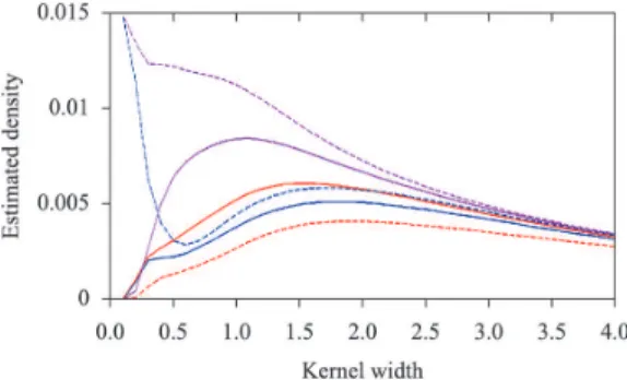
As seen in Figure 6, the decision criterion of Equation 17 leads to consistency in the behavior of the densities with respect to h.The direct minimization of the sum of the densities of all points, for example, may not be a good decision criterion because the density values may differ from the values observed in the graph. The decision criterion of Equation 17 guarantees a condition of minimum coherence for the values of the densities at the midpoints, that is, the approximation function tends to smoothness at all midpoints.
Experimental Stages
The experiments performed in the present work may be divided into two stages, which will be presented below.
Data modeling and selection of the Kernel Width h
After normalization of the data to use the kernel width estimated by the proposed method for all data variables, the midpoints between the classes are calculated. At the midpoints, the density is calculated for different width values of a Gaussian kernel, as seen in Figure 6.
The method for choosing h considers the behavior
of the densities for the utilized value of the width. The goal is to avoid small width values, which lead to complex separation curves that are over itted to the data; these types of curves have little generalization power. Similarly, large values should be avoided because they produce overly smooth responses of the model. Therefore, the chosen h is the one for which
the derivative at all midpoints is negative, indicating
Figure 6. Density variation at the margin points with respect to the
that the density curves downward, as described in Equation 17.
Classiication and performance analysis with respect to Width
After the kernel width estimation, the performance of the resulting model is compared with the performance of the method proposed by Silverman (1986). For this comparison, the KDE-Bayes method (Wanderley et al., 2010), which consists of a probabilistic classiier based on Bayes Theorem, was used. This method is divided into two stages: the non-parametric density estimation for each class (KDE stage) and data classiication using the Bayesian decision rule and the densities of the irst stage (Bayes stage).
The performance of the classiier for each value of width is then evaluated according to three metrics: accuracy (Ac), speciicity (Sp) and sensitivity (Se). Next, an analysis of variance (ANOVA) is performed to determine whether the means of each metric are substantially different.
Databases
For this work, the experiments were conducted using two types of databases. The initial tests, using 7 public databases (Table 1) from the University of California, Irvine (http://archive.ics.uci.edu/ml/), were performed to verify the behavior of the proposed method.
Next, experiments were conducted on genetic expression data from tumor cancer cells (available at http://bioinformatics.mdanderson.org/pubdata. html). The clinical trial was conducted at the Nellie B. Connally Breast Center, M.D. Anderson Cancer Center, University of Texas (Hess et al., 2006). Data were collected from 82 patients in Houston, USA and 51 patients in Villejuif, France; all patients had breast cancer that was between stages I – III. Before the beginning of the neoadjuvant treatment, samples from the tumor were collected by ine needle aspiration. By the end of the treatment, all patients underwent surgeries for tumor bed resection to determine whether the pathologic response was complete. For each patient, 22283 probes were obtained from the genetic
expression of tumor samples using a microarray technique.
For each dataset, 100 repetitions of 3-fold cross validation were made in which the performance was analyzed for the kernel width proposed by Silverman (1986) and for the method proposed in this paper that considers that maximum margin between classes. To train the model, 2/3 of the data from the 7 public databases was used, and the other 1/3 of the data was used for the test. For the neoadjuvant chemotherapy, the data from Houston were used for training, and the data from Villejuif were used for the test. The results were evaluated according to mean and standard deviation of the accuracy, sensibility and speciicity, which were calculated from the results for each repetition of cross validation. For a statistical comparison of the results obtained with KDE-Bayes for each of the proposed h values, an analysis of variance (ANOVA) was performed on the means of the metrics used for evaluating the performance of the width h.
Results
All databases
Table 2 presents the results of the KDE-Bayes classiier for the proposed width using this work (Ac, Sp, Se, Ac Test, Sp Test, Se Test) and using the method of Silverman (Acs, Sps, Ses, Acs Test, Sps Test, Ses Test). The values shown in the table are the mean and standard deviation of the results obtained for cross validation executions using the training and test sets.
Bioinformatics
Similarly, Table 3 presents the results for the problem of predicting the effectiveness of the neoadjuvant chemotherapy for the breast cancer patients. The indicated metrics and values are the same as those used for the experiments presented in Table 2.
Discussion
The analysis of variance (ANOVA) (Scheffé, 1959) using the results presented in Tables 2 and 3 indicated statistical equivalence between the values obtained using the two methods of estimating kernel width: the method proposed in this paper and the one proposed by Silverman (1986). These results support the goal of this work, which is discussed in the Methods section, and indicate that the data labeling and the function that generates the data are consistent. Although the results are statistically equivalent, the performances Table 1. Summary of the UCI Datasets that were used.
Name No. of
characteristics Class 1 Class 2
ACR 14 383 307
BLD 6 145 200
ION 33 225 126
SNR 60 97 111
TTT 9 626 332
WBC 9 444 239
for the larger and smaller classes are better balanced using the proposed method, while Silverman’s method performs better for the large class.
For predicting the effectiveness of neoadjuvant chemotherapy (Table 3), the two methods have similar performance using the training set; however, the proposed method is slightly superior with the test set. Because this problem aims to determine whether patients should be treated before surgery, the number of false negatives should be as small as possible, even
if the number of false positives is slightly larger. The value of h proposed by Silverman misses 36% of the
cases, compared with 30% for the value selected in the present study.
Because the presented method is based on the existence of a low density region between classes, it has some limitations. This method is mainly applicable to binary classiication problems because of its dificulty in determining the separation margin for three or more classes. Similarly, it is Table 2. UCI Datasets: results of 3-fold cross validation using the kernel width chosen by the proposed method (error limited on 0.05) and
the width chosen the method of Silverman. Ac = Accuracy, Sp = Speciicity, Se = Sensitivity, Acs = Accuracy Silverman, Sps = Speciicity Silverman, Ses = Sensitivity Silverman.
ACR
Ac Sp Se Ac Test Sp Test Se Test
0.993 ± 0.002 0.999 ± 0.001 0.986 ± 0.004 0.802 ± 0.010 0.837 ± 0.016 0.759 ± 0.009
Acs Sps Ses Acs Test Sps Test Ses Test
0.986 ± 0.002 0.999 ± 0.002 0.970 ± 0.006 0.819 ± 0.011 0.859 ± 0.012 0.769 ± 0.015
BLD
Ac Sp Se Ac Test Sp Test Se Test
0.980 ± 0.006 0.975 ± 0.010 0.983 ± 0.009 0.631 ± 0.016 0.529 ± 0.043 0.705 ± 0.027
Acs Sps Ses Acs Test Sps Test Ses Test
0.901 ± 0.010 0.812 ± 0.027 0.966 ± 0.006 0.636 ± 0.025 0.442 ± 0.049 0.777 ± 0.028
ION
Ac Sp Se Ac Test Sp Test Se Test
0.997 ± 0.001 0.996 ± 0.001 0.999 ± 0.003 0.862 ± 0.012 0.983 ± 0.007 0.646 ± 0.024
Acs Sps Ses Acs Test Sps Test Ses Test
0.996 ± 0.002 0.998 ± 0.001 0.992 ± 0.000 0.882 ± 0.009 0.988 ± 0.006 0.694 ± 0.032
SNR
Ac Sp Se Ac Test Sp Test Se Test
1.000 ± 0.000 1.000 ± 0.000 1.000 ± 0.000 0.847 ± 0.013 0.792 ± 0.035 0.895 ± 0.030
Acs Sps Ses Acs Test Sps Test Ses Test
1.000 ± 0.000 1.000 ± 0.000 1.000 ± 0.000 0.842 ± 0.013 0.785 ± 0.031 0.892 ± 0.035
TTT
Ac Sp Se Ac Test Sp Test Se Test
1.000 ± 0.000 1.000 ± 0.000 1.000 ± 0.000 0.883 ± 0.010 1.000 ± 0.000 0.662 ± 0.030
Acs Sps Ses Acs Test Sps Test Ses Test
1.000 ± 0.000 1.000 ± 0.000 1.000 ± 0.000 0.921 ± 0.007 1.000 ± 0.000 0.771 ± 0.020
WBC
Ac Sp Se Ac Test Sp Test Se Test
0.996 ± 0.002 0.998 ± 0.004 0.993 ± 0.004 0.957 ± 0.005 0.977 ± 0.005 0.921 ± 0.014
Acs Sps Ses Acs Test Sps Test Ses Test
0.991 ± 0.001 1.000 ± 0.000 0.975 ± 0.003 0.961 ± 0.005 0.976 ± 0.004 0.933 ± 0.014
HEA
Ac Sp Se Ac Test Sp Test Se Test
1.000 ± 0.000 1.000 ± 0.000 1.000 ± 0.000 0.782 ± 0.019 0.803 ± 0.026 0.757 ± 0.033
Acs Sps Ses Acs Test Sps Test Ses Test
0.999 ± 0.002 1.000 ± 0.000 0.997 ± 0.004 0.788 ± 0.018 0.807 ± 0.025 0.764 ± 0.022
Table 3. Breast Cancer Problem: results of 3-fold cross validation to the kernel width chosen by the proposed method (error limited on
0.05) and the width chosen by the method of Silverman. Ac = Accuracy, Sp = Speciicity, Se = Sensitivity, Acs = Accuracy Silverman, Sps = Speciicity Silverman, Ses = Sensitivity Silverman.
Ac Sp Se Ac Test Sp Test Se Test
1.000 ± 0.000 1.000 ± 0.000 1.000 ± 0.000 0.753 ± 0.039 0.783 ± 0.032 0.668 ± 0.064
Acs Sps Ses Acs Test Sps Test Ses Test
also dificult to use semi-supervised learning for cases in which the class is composed of two or more clusters, which could be considered a multiple class problem.
The results support the proposed hypothesis: this work provides an alternative to model selection and is based on the problem geometry and the known labels for each class.
The principle that the separation region is located in a low density area has been used in other studies to guide the construction of large margin classiiers. This principle suggests that the maximum margin separator and the minimum error of the inductive data set should be located in a region of low density. Although this is the general principle of large margin classiiers, such as SVMs, the densities at separation points are not directly calculated. Generally, a region of low density is identiied as the result of the maximization of the separation margin through an objective function that is associated with the magnitude of the parameters (weights) of the model. In this work, however, an approach was presented that aimed to irst identify the low density region that would be used for the selection criterion to obtain an adequately smooth separation surface, thus leading to a large margin separator. By constructing appropriate kernel matrices and geometrically identifying the separation midpoints through the Gabriel graph, objective functions for minimizing the classiication error were described. The smoothness of the response of the minimum error model is obtained by utilizing a selection method that is based on calculating the densities at the midpoints. The inal model was evaluated using several databases and was shown to be robust for the test set, suggesting that a good balance between bias and variance is obtained indirectly through the selector based on the densities calculation. The results are compatible with the ones obtained by methods that explicitly control the bias and variance, such as the one proposed by Silverman (1986). Many of the results are within the limit of the benchmarking for the databases that were used for the tests. This work was not designed to develop a new methodology that outperforms the current methods, which may not even be possible for the used databases. Thus, in this work, a new method was described; this method was capable of selecting models using direct density calculations and the geometry of the separation problem. Focusing on the point densities instead of the direct calculation of the separation margin is a viable alternative for constructing generative models of separation.
Acknowledgements
This work was supported by CNPq, Conselho Nacional de Desenvolvimento Cientíico e Tecnológico – Brazil.
References
Chapelle O, Schölkopf B, Zien A. Semi-supervised learning. MIT Press Cambridge; 2006. http://dx.doi.org/10.7551/ mitpress/9780262033589.001.0001
Cortes C, Vapnik V. Support vector networks. Machine Learning. 1995; 20(3):273-97. http://dx.doi.org/10.1007/ BF00994018
De Berg M, Cheong O, Van Kreveld M, Overmars M. Computational geometry: algorithms and applications. Springer; 2000.
Geman S, Bienenstock E, Doursat R. Neural networks and the bias/variance dilemma. Neural computation. 1992; 3(1):1-58. http://dx.doi.org/10.1162/neco.1992.4.1.1
Hess KR, Anderson K, Symmans WF, Valero V, Ibrahim N, Mejia JA, Booser D, Theriault RL, Buzdar AU, Dempsey PJ, Rouzier R, Sneige N, Ross JS, Vidaurre T, Gómez HL, Hortobagyi GN, Pusztai L. Pharmacogenomic predictor of sensitivity to preoperative chemotherapy with paclitaxel and luorouracil, doxorubicin, and cyclophosphamide in breast cancer. Journal of Clinical Oncology. 2006; 24(26):4236-44. PMid:16896004. http://dx.doi.org/10.1200/JCO.2006.05.6861 Johnson SC. Hierarchical clustering schemes. Psychometrika. 1967; 32(3):241-54. PMid:5234703. http:// dx.doi.org/10.1007/BF02289588
Okabe T, Jin Y, Sendhoff B. A critical survey of performance indices for multi-objective optimisation. In: CEC 2003: Proceedings of the IEEE Congress on Evolutionary Computation; 2003 Dec 8-12; Canberra, Australia. Canberra; 2003. p. 878-85.
Parzen E. On estimation of a probability density function and
mode. Annals of Mathematical Statistics. 1962; 33(3):1065-76. http://dx.doi.org/10.1214/aoms/1177704472
Queiroz FAA, Braga AP, Pedrycz W. Sorted kernel matrices as cluster validity indexes. In: Carvalho JP, Dubois D, Kaymak U, Sousa JMC, editors. Proceedings of the Joint 2009 International Fuzzy Systems Association World Congress and 2009 European Society of Fuzzy Logic and Technology Conference; 2009 Jul 20-24; Lisbon, Portugal. Lisbon; 2009. p. 1490-5.
Scheffé H. The analysis of variance. Wiley; 1959. Scott DW. Multivariate density estimation. Wiley Online Library; 1992. http://dx.doi.org/10.1002/9780470316849 Scott GL, Longuet-Higgins HC. Feature grouping by relocalisation of eigenvectors of the proximity matrix. Proceedings of British Machine Vision Conference; 1990. p. 103-8. PMid:2313271.
Teixeira RA, Braga AP, Takahashi RHC, Saldanha RR. Improving generalization of MLPs with multi-objective optimization. Neurocomputing. 2000; 35(1):189-94. http:// dx.doi.org/10.1016/S0925-2312(00)00327-1
Torres LCB, Castro CL, Braga AP. A computational geometry
approach for pareto-optimal selection of neural networks. In: ICANN 2012: Proceedings Artiicial Networks and Machine Learning; 2012 Sep 11-14; Lausanne, Switzerland. Lausanne; 2012. p. 100-7.
Van Gestel T, Suykens JAK, Baesens B, Viaene S, Vanthienen J, Dedene G, De Moor B, Vandewalle J. Benchmarking least squares support vector machine classiiers. Machine
Learning. 2004; 54(1):5-32. http://dx.doi.org/10.1023/ B:MACH.0000008082.80494.e0
Vapnik V. The nature of statistical learning theory. Springer; 1999.
Wanderley MFB, Braga AP, Mendes EMAM, Natowicz R,
Rouzier R. Non-parametric kernel density estimation for the prediction of neoadjuvant chemotherapy outcomes. In: Annual International Conference of the IEEE 2010: Proceedings Annual International Conference of the IEEE; 2010 Aug 31-Sep 4; Buenos Aires, Argentina. Engineering in Medicine and Biology Society - EMBC; 2010. p. 1775- 8. PMid:21096419.
Authors
Maria Fernanda Barbosa Wanderley*, Luiz Carlos Bambirra Torres
Graduate Program in Electrical Engineering, Federal University of Minas Gerais – UFMG, Av. Antônio Carlos, 6627, CEP 31270-901, Belo Horizonte, MG, Brazil.
René Natowicz
ESIEE-Paris, University of Paris-Est, Noisy-le-Grand, France.
Antônio Pádua Braga
Erratum
In the article “A maximum margin-based kernel width estimator and its application to the response to neoadjuvant chemotherapy”, DOI http://dx.doi.org/10.4322/rbeb.2014.007, published in Revista Brasileira de Engenharia Biomédica (previous title of the Research on Biomedical Engineering Journal), v. 30 n. 1, p. 17-26, 2014, on page 25,
Where it reads:
“Acknowledgements
This work was supported by CNPq, Conselho Nacional de Desenvolvimento Cientíico e Tecnológico - Brazil.”
It should be read:
“Acknowledgements
![Figure 1. Bidimensional data sampled from ive distinct distributions with means m 1 = [1, 4], m 2 = [3, 4], m 3 = [4, 4], m 4 = [2, 2], and m 5 = [4, 2] and standard deviation 0.3.](https://thumb-eu.123doks.com/thumbv2/123dok_br/18855764.416886/2.765.371.659.770.1003/figure-bidimensional-sampled-distinct-distributions-means-standard-deviation.webp)

![Figure 4. Data sampled from two Gaussian distributions with means m 1 = [2, 2] T and m 2 = [4, 4] T .](https://thumb-eu.123doks.com/thumbv2/123dok_br/18855764.416886/4.765.372.659.103.361/figure-data-sampled-gaussian-distributions-means-t-t.webp)