en 0104 530X gp 0104 530X2288 15

http://dx.doi.org/10.1590/0104-530X2288-15

Resumo

Neste estudo, considera-se um problema de dimensionamento e programação de lotes de produção de bebidas não alcoólicas à base de frutas. O problema é caracterizado por horizonte de planejamento com múltiplos períodos, processo de produção com máquinas distintas, restrições de capacidades de produção e tempos de preparação das máquinas independentes da sequência de produção, além de condições especiais de preparações, como limpezas obrigatórias das máquinas dentro de limitações de tempo de produção. Para tratar o problema, propõe-se uma abordagem de solução baseada em modelos de programação matemática e uso de softwares de otimização. Os modelos são modiicações de modelos de programação linear inteira mista conhecidos na literatura de dimensionamento e programação de lotes de produção. Porém, ao invés de considerar múltiplas máquinas em paralelo, os modelos propostos exploram outras possíveis conigurações de máquinas para representar apropriadamente os processos de produção envolvidos na produção de bebidas à base de frutas. A abordagem proposta é validada por meio de um estudo realizado em uma fábrica de sucos e néctares de frutas no interior do Estado de São Paulo, em que as soluções obtidas pelos modelos foram testadas e analisadas em situações realistas da empresa. Os resultados mostram que a abordagem tem bom potencial de aplicação prática.

Palavras-chave: Indústria de bebidas não alcoólicas; Planejamento da produção; Programação inteira mista; Dimensionamento de lotes.

Abstract

This study considers a production lot-sizing and scheduling problem of non-alcoholic fruit juice beverages. The problem is characterized by a multi-period planning horizon, a production process with different machines, capacity constraints and setup times independent from the production sequence, as well as special conditions regarding required machines clean-in-place (CIP) within production time periods. To deal with this problem, we propose a solution approach based on mathematical programming and using optimization software. The models are modiications of mixed integer programming models known in the lot sizing and scheduling literature. However, instead of considering multiple parallel machines, the proposed models explore other possible conigurations of machines to properly represent the production processes involved in producing fruit beverages. The proposed approach is validated by a study carried out in a fruit juice company located in the interior of Sao Paulo State, Brazil, in which the solutions obtained by the models were tested and analyzed in real situations at the company. The results show that the approach is potentially good for practical applications.

Keywords: Non-alcoholic fruit juice beverage industry; Production planning; Mixed integer programming; Lot sizing and scheduling problem.

Optimizing the production scheduling of fruit juice

beverages using mixed integer programming models

Otimização da programação da produção de bebidas à base de frutas por meio de modelos de programação inteira mista

Marina Sanches Pagliarussi1

Reinaldo Morabito1

Maristela Oliveira Santos2

1 _{Departamento de Engenharia de Produção, Universidade Federal de São Carlos – UFSCar, Rod. Washington Luiz, Km 235,}

CEP 13565-905, São Carlos, SP, Brazil, e-mail: mari.paglia@gmail.com; morabito@ufscar.br

2 _{Instituto de Ciências Matemáticas e de Computação, Universidade de São Paulo – USP, Av. Trabalhador São-Carlense, 400,}

CEP 13560-970, São Carlos, SP, Brazil, e-mail: mari@icmc.usp.br Received May 15, 2015 - Accepted Nov. 15, 2015

Financial support: CAPES, CNPq and FAPESP.

1 Introduction

Over the last few years, there has been a signiicant growth in the production of non-alcoholic drinks in Brazil

(ABIR, 2010; Diário Econômico, 2011). The potential increase in the consumption of these products, the

growth of the number of items manufactured by the industry, as well as the competition and demands of

this market has resulted in companies being concerned

in areas directly involved with production, such as production planning and control. In 2015, it was estimated that there will be a growth in the production

of the entire drink sector, according to the Beverage

Production Control System - SICOBE (SICOBE, 2005). One of the recurrent challenges in this sector

is to obtain eficient production programs, which

should consider the time available for production, the input availability, the demands of every period, the machines to be set up and the changeovers between

items to be produced. It is also important to take into

consideration the synchrony between the two main

production phases: preparing syrups and packaging beverages. Some studies about non-alcoholic drink companies in Brazil, more speciically concerning the production of soft drinks and other carbonated drinks

(Toledo et al., 2007; Ferreira et al., 2009) and fruit

juice drinks highlight the dificulty in determining

effective production plans (generally manually). During the development of this research, various visits to typical companies of the beverage industry in the State of São Paulo were made. During these visits, the production managers and programmers of

these companies reafirmed the dificulty in taking

lot sizing and scheduling decisions. Such challenges

were also observed in fruit juice drink production lines, which are the object of this study. Having the

collaboration of these companies, we chose one of these lines in order to meet the objectives of this study. The selected company has typical characteristics of other production lines of beverage companies.

The fruit-based drink production line was selected because this type of drink has shown increasing trends

over recent years (ABIR, 2010). The consumption

of ready-to-drink fruit-based beverages is still below the consumption of soft drinks. On the other hand,

this is seen by some authors as an indication of its growth potential (Pirillo & Sabio, 2009).

The lot sizing and scheduling problem in the fruit juice beverage industry consists of determining the lot size of different types of fruit juices (items) to

meet the demands in each period of a inite planning

horizon. Each beverage production line has its own characteristics. In the fruit juice line studied in this

work, the setup time, for instance, is not sequence dependent, unlike other beverage production lines. In most studies, such as in carbonated drinks, the

setup operations in the production lines are widely dependent on the sequence of production (Toledo et al., 2007; Ferreira et al., 2009). In addition, in fruit juice

production, tanks and illing machines must be cleaned

within production time constraints. It is mandatory to clean the lines (this is called CIP - Clean-in-Place) after a certain time of production, regardless of whether

there is change of beverage lavor or not in the fruit juice line. If there is a change of lavor (item), the

same cleaning is required, and the cleaning time does

not vary with the lavor of the product. A preliminary

study in a fruit juice production line can be found in Leite (2008), where machine setups do not depend on the result of production batches.

The lot sizing problem and its extensions have been

widely investigated by the scientiic community and

by consultants related to businesses, motivated by applications in industrial environments. Comprehensive reviews about lot sizing can be found in Drexl & Kimms (1997), Karimi et al. (2003), Jans & Degraeve

(2008), Buschkühl et al. (2010) and Glock et al.

(2014). Among the lot sizing models, linear models such as the Capacitated Lot Sizing Problem (CLSP)

and the General Lot Sizing and Scheduling Problem (GLSP) stand out. CLSP is characterized by being big bucket, meaning that several items can be produced in

each period. The problem considers that the limited resources are used for production and to set up machines. The CLSP with capacity constraints and setup times can be found, for example, in Trigeiro et al. (1989).

The GLSP was proposed by Fleischmann & Meyr

(1997) and Meyr (2002). It consists of determining lot sizes of several products and scheduling them in a single machine or parallel machines subject to capacity constraints. Each macro period is divided into smaller periods called micro periods. The duration of each micro period is so short that only one type

of item can be manufactured in it. Hence, we obtain

the sequence in which each item should be produced in each macro period.

The lot-sizing and scheduling problems have been widely used in several productive sectors (e.g., Araujo et al., 2008; Almada-Lobo et al., 2008; Luche et al., 2009; Toso et al., 2009; Santos & Almada-Lobo, 2012; Marinelli et al., 2007; Kopanos et al., 2010, among many others). Some studies are found

in the production of non-alcoholic drinks such as soft drinks, water, tea and juice, but most of these studies consider soft drink production lines. For example,

Toledo et al. (2007) presented an integrated model

for a lot sizing and scheduling problem in a soft drink industry based on the GSLPPL (GSLP with parallel

machines) from Meyr (2002). The production involves two interdependent levels with decisions concerning the storage of raw materials and bottling beverages. The aim was to determine the design and programming

of raw materials in the tanks to produce syrups and bottle packaging in the lines where times and costs

depend on the type of item previously stored and

packaged. In the bottling lines, the setup time and

cost depend on the type of previously stored and bottled item. Other related studies can be found in Toledo et al. (2009, 2014, 2015).

Clark (2003) explores several heuristic solution

approaches for a mixed integer programming model, based on the CLSP, to address the production problem

and the process of illing the mixed liquid in cans

was chosen for a pilot project. In Rangel & Ferreira (2003), a mixed integer programming model is also

developed, nonetheless based on GLSP, for a lot sizing and scheduling problem in a soft drink company with

sequence-dependent setup costs and setup times. In Ferreira et al. (2009), these studies have been

extended to deal with cases in the soft drink industry with several illing lines and with several available tanks to prepare syrups. Regarding the problem, the production bottleneck alternates between the liquid

preparation stage and the bottling one, therefore synchronization of the production between these stages is required. Other related studies appear in Ferreira et al. (2010, 2012) and Defalque et al. (2011).

Leite (2008) is the only study found in the literature review that deals with the production problem of a line of fruit beverages. A preliminary study was

conducted in a beverage industry to ind out about

the particularities of the production lines involved, and a model based on Ferreira et al. (2009) and the

GLSP were developed to analyze it. In this study, three identical illing machines serviced by a single tank were identiied. Thus, the three machines can ill only one type of drink lavor at a time.

In this paper, we consider a lot sizing and scheduling problem in beverage plants which produce fruit beverages with some similarities to the problem

studied in Leite (2008). However, although the

characteristics of the product are the same (with setup time and setup cost that are non-dependent from the production sequence), the attributes of the production line are different as the process is different

and involves various illing machines and more tanks, mixers and pasteurizing, as presented below. In this paper, the illing machines will be presented as packaging machines for the sake of simpliication.

The problem is initially represented by a mathematical

model based on GLSPPL (Meyr, 2002), used to avoid

the problem of maximum lot sizes in these types of companies, due to mandatory cleaning within production time constraints. The obtained solution by the model consists of determining the lot sizes of items and the production sequence, however these lots can be interchanged within each period without loss of generality, due to the fact that the setup is sequence independent of the production of the items. Considering the previous model, a simpler model is developed to represent the problem based on the CLSP. This new model also considers all characteristics of the production process such as mandatory cleaning,

but simpliies decisions about scheduling lots. Both

models are solved by CPLEX software using generated examples based on realistic data from the company

with planning horizons of a few weeks.

The structure of the paper is as follows. The next

section briely describes the production process of

fruit beverages according to the reality of the studied company and also provides information about how the production planning is carried out in this company. The proposed mathematical models are presented in Section 3. The computational results are described in Section 4. Finally, in Section 5, the conclusions and perspectives for future research are discussed.

2 Production process

This research was supported by the cooperation of a factory in São Paulo. This factory produces soft

drinks and fruit juice drinks. The need for a more

effective production planning technique was observed due to the demand and type of product, especially on the line related to the group of non-carbonated and

fruit juice products. This line is the market leader

in its sector, and in this study it is renamed Line 1.

Line 1 produces ive different lavors of fruit juice drinks (pineapple, orange, passion fruit, strawberry

and grape) and it is different from the other lines of the factory due to the fact that its setup time is sequence

independent, unlike the soft drink lines, for example.

On the other hand, the product has characteristics

whereby the tanks and bottling machines need to

be cleaned every 48 hours, which is not absolutely

necessary for the other drinks. The cleaning process

consists of different cycles that are recirculated through

the tanks, pumps, valves and other equipment in the process low. It is important to note that once the

line has been cleaned, production should be started as soon as possible because the line is not perfectly hermetic. Production can be continuous, which means the production can be resumed in the last period.

The production of drinks generally has two main stages: liquid lavor preparation and bottling (packaging). In the irst stage, the main raw material, the liquid lavor or syrup, is prepared in tanks of different capacities. The tanks should work with a

minimum liquid quantity to ensure its homogeneity.

To properly mix the necessary ingredients, the tank

propeller must be completely covered. In the second stage, the liquid is bottled in the production lines. A production line is made up of a conveyor belt

and machines that wash the bottles, ill them with a combination of liquid lavor and water (carbonated or non carbonated) and then seal, label and pack them.

The two stages are shown in Figure 1. The syrup and water are put into the mixer in order to homogenize the two components. The mixture is then put into

the preparatory tank and, afterwards the buffer tank. The preparatory tank and the buffer tank maintain

the mix homogeneous as both have helixes at the

constantly provided by the preparatory tank. It takes approximately two hours to ill the preparatory tank for the irst time and ifty minutes to ill the buffer. After that, the supply is constant. The bottleneck of this line production is the packaging machines.

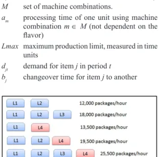
In Figure 1, the four packaging machines are called L1, L2, L3 and L4.

It can be observed in Figure 1 that the preparatory

tank has a capacity of 12m3 _{and it supplies two buffer}

tanks with capacities of 12 m3 each. Buffer tank 1 only

serves the L1, L2 and L3 machines, each one with a

packaging capacity of 6,000 packages per hour, and buffer tank 2 supplies the L4 machine, with a capacity of 7,500 packages per hour. Pasteurizers 1 and 2 shown in the igure, whose function is to destroy bacteria,

have various capacities. The maximum capacities

are 18,700 packages per hour and 32,500 packages

per hour, respectively. On the other hand, these maximum capacities are not reached because the L1, L2 and L3 machines have total nominal capacities of

18,000 packages per hour. The cleaning process of these packaging machines is generally simultaneous and it always takes more time than cleaning the tanks, therefore when the machines are ready to work, the buffer tank will be full.

In this study, we also studied a change in the productive process described in Figure 1 including

a new bottling machine, called L5, with a packaging capacity of 11,200 packages per hour, supplied by

buffer 2 with machine L4. Buffer 2 also supplies the L4 machine. This process with the L5 machine went into the adaptation phase in the company while developing this study, therefore it is also considered

in the study. However, not all the combinations of the

machines are feasible for operation in Figure 1 or in the

second coniguration of this production process with

machine L5. For example, with a limited capacity, it is

not feasible to produce less than 12,000 packages/hour,

which means that at least two of the machines L1, L2 or L3 must be connected (if machines L4 and L5 are off). Similarly, it is not feasible to produce only using machine L4 or at least machine L5 connected (if machines L1, L2 and L3 are turned off), both with

smaller capacities than 12,000 packages/hour. As can be seen, buffer tank 1 supplies the L1, L2 and L3 packaging machines, and buffer 2 supplies the

L4 machine as shown in Figure 1 and the L4 and L5

machines in the modiied coniguration. It is worth mentioning that although the buffer tanks have the same

capacity, the capacities of the pasteurizers are different: the pasteurizer connected to machines L1, L2 and L3

have a maximum capacity to process 18,700 packages

of 200 ml per hour, while the pasteurizer connected to machines L4 and L5 have a processing capacity

of 32,500 packages per hour. The washing process of

all the machines is generally done at the same time

and takes four hours. According to the production programmer, it would take approximately two hours

to clean only one machine, while the cleaning time of all the machines is four hours. Therefore, there was no reason to carry out the washing process in only one machine at a time.

The buffer tanks supply two different groups of packaging machines. Once we consider that the capacity of the tanks is large enough for the purposes

of scheduling the production, the problem considered in this article can be considered as single-stage, considering that there is always enough syrup to

supply the packaging machines. Hence, we approach

the problem of lot sizing and scheduling the fruit

based drinks considering a mixer and a preparatory tank that supply two buffers as shown in Figure 1.

The production scheduling in the company is done manually. The demand data of the 5 products are obtained through a second company (which is a partner to the same business group) that purchases products made by Line 1. Considering the demand data, the production programmer distributes the

obtained demand of the month in weeks. These

demand data are shared with the liquid preparation sector. These amounts are then passed to the syrup

sector, which calculates the amount of kits needed to

meet the demand. A relevant feature of Line 1 is that production lots generally last 48 hours. Production

lexibility is achieved by changing the number of

machines designated to that “batch” and by the speed

of the pasteurizer. Stock quantities do not interfere

in the production planning.

The stock created by the production planning is

controlled by a partner of the business group that

monitors the stock levels and labor distribution in the factory. Therefore, the task of optimizing lot sizing and scheduling is not affected by stock numbers.

Consequently, the product programmer aims to meet the demand considering setup times without

backlogging, but with no focus on inventory. On the

other hand, it is advantageous to schedule lots that last at least 48 hours in order to avoid unnecessary setups.

The lexibility of the lot size production consists of sending one of the packaging machines for maintenance

and reducing the speed of the pasteurizer, so that

the product is not wasted by excessive cooking.

Therefore, this results in the lot of 48 hours having a lower number of products. The programmer forwards the schedule to the production line supervisor, who

places the quantities in lots of 48 hours. However,

it is not always possible to meet the demand in lots

of 48h. In this case, the production supervisor asks

for the lowest nearest multiple demand and consults the programmer about the possibility of producing another lot.

Fractions of kits can be used in the plant, which

is the measurement of syrup used. The minimum

fraction is pre-set at 0.25 kit, as there must be a minimum amount of liquid in the tank so that the helix for the mixture can rotate. However, the fraction

normally used by the production programmer is

0.5 kit, except for the strawberry and orange lavors.

The correspondences can be seen in Table 1. These

fractions are used because the tanks have a capacity

of 12m3_{. If the calculated amount does not provide}

a whole number of fractions of kits or batches, the manager in charge of the syrup makes the largest

whole number of batches contained in the calculated

amount and consults the scheduler about making one

more batch to cover the fraction or leave it for the

following week, i.e. rounding it up or down.

For example, consider that the programmer sent a

production of 120,000 boxes of grape lavor, which is

equivalent to 12×120×103 _{units of 200mL = 1,440,000}

packages of grape lavored drinks (288,000 liters)

to the manager in charge of the syrup. According to Table 1, 14.4 kits would be needed. In this example, the manager in charge of the syrup would

consult the programmer to know if they would use 14.5 or 14 kits of the grape lavor. In batches, this

would mean 29 or 28 batches, respectively. For details

of this fruit drink production process, please consult

Pagliarussi (2013).

3 Problem modeling

In this section, the one-stage models to represent

the fruit juice drink production planning are described. Model I is based on GLSPPL and Model II is based

on CLSP. Model I can approach the production problem in order to maximize the contribution margin

or minimize inventory, backlogging and setup costs.

The two approaches are respectively called Model

Ia and Model Ib. Model Ia is proposed taking into

consideration the suggestions made by the company´s production manager, whilst Model Ib is more common in the lot sizing literature.

The main difference between Models Ia and Ib is the objective function. Model II also aims at minimizing production costs, similar to Model Ib. Model solutions can be interpreted as feasible production plans, optimizing a given criteria and providing lot sizes

Table 1. Flavor, batch and kit proportion.

Flavor

Amount produced by

kit (L)

Batch (kit fraction)

Orange 12,000 1

Grape 20,000 0.5

Passion fruit 24,000 0.5

Pineapple 24,000 0.5

of each drink lavor in order to meet demands. Every model presented in this study takes into consideration

sequent independent setup times.

It is mandatory to consider that it takes at least two packaging machines to make production viable

in Line 1, such as shown in Figure 1. Therefore, in the following mathematical models, we consider parameter M as the set of all possible combinations of

operating machines. Taking Figure 1 as an example, where machines L1, L2, L3 and L4 are presented, the viable combinations are shown in Figure 2. Every combination represents machines for which

the sum of the packaging capacity is equal or more than 12,000 packages per hour. Other combinations including machine L5 are deined similarly. Since

machines L1, L2 and L3 are equal, some of the combinations are symmetric and can be left out (i.e. any combination regarding two of the following L1, L2 or L3), without loss of generality. Thus, the cardinality of set M is 5, that is: M ={(L1,L2); (L1,L2,L3); (L1,L4); (L1,L2,L4); (L1,L2,L3,L4)}.

Another aspect that should be taken into consideration

when developing models is the synchronization of production machines. According to the production

programmer, all machines start working at the same time. However, there may be some breaks or pauses

during the production runtime. L1, L2 and L3 are synchronized machines most of the time as they are connected to the same pasteurizer, but the timing of L4 and L5 machines with L1, L2 and L3 is adopted in

the model as a combination for the sake of simplicity.

The model parameters and data inputs are:

T number of micro periods, t∈ T J number of liquid lavors, j∈ J

S_t set of micro periods in each period t, s∈ S_t M set of machine combinations.

a_m processing time of one unit using machine combination m∈ M (not dependent on the

lavor)

Lmax maximum production limit, measured in time units

d_jt demand for item j in period t

b_j changeover time for item j to another

q_j minimum lot size of lavor j to ensure the liquid homogeneity

Kt total time capacity in period t

3.1 Model I

Model I is based on the GLSPPL model (Meyr, 2002), but with some modiications in order to

include the maximum production constraint. Model I represents a situation where there is one preparatory

tank linked to two buffer tanks, connected to both

pasteurizers. After the pasteurization process, the next

stage is packaging, using machines L1, L2 and L3

connected to pasteurizer 1 and machines L4 and L5

connected to pasteurizer 2. At irst, in this study,

information obtained in the factory was used, such

as not taking into consideration either inventory costs or idle machine costs. Backlogging costs were not available at that time. Hence, the fruit juice based drink production planning can be stated as follows. Deine the lot sizes and production scheduling taking into account the fruit juice drink demands and the capacity of packaging machines, so that the proit

margin is maximized (Model Ia), as suggested by the factory production manager. Afterwards, we altered the objective function in order to minimize the overall costs, which is discussed further (Model Ib)

Model Ia - additional parameters

p_j proit margin of item j

Variables

x_jmts production quantity of item j in machine combination m in micro period s of period t; I_jt inventory for item j at the end of period t; z_jmts 1, if item j is produced in machine combination

m during micro period s of period t; 0, otherwise.

Model Ia

max _jmts

j j J m M t T s St∈ ∈ ∈ ∈

p x

∑ ∑ ∑ ∑

Subject to:

( 1) ,

t

j t jmts jt jt

m M s S

I − x I d j J t T

∈ ∈

+

∑ ∑

,

t t

m jmts j jmts t

m M j J s S m M j J s S

a x b z K t T

∈ ∈ ∈ ∈ ∈ ∈

+ ≤ ∀ ∈

∑ ∑ ∑

∑ ∑ ∑

, , , ,

jmts

jmts

q

x

z

1 , , jmts

m M j J

s St t T

z

∈ ∈

≤ ∀ ∈ ∀ ∈

∑ ∑

Figure 2. Viable combinations considering four packaging

max

, , ,

jmts jmts

m L

j J m M s St t T

x

z

a

 

≤_ _ ∀ ∈ ∀ ∈ ∀ ∈ ∀ ∈

 

, (6)

{ }0,1 , 0, 0, , , ,

jmts xjmts jt j J m M s St t T

z ∈ ≥ I ≥ ∀ ∈ ∀ ∈ ∀ ∈ ∀ ∈ . (7)

The objective function (1) maximizes the total contribution margin. Constraints (2) are the inventory balance equations and together with Ijt≥0, for all j

and t, they ensure that the demand is met without

backlogging. Constraints (3) represent the capacity

constraints in each period, that is, the time spent on production and on setup cannot exceed the available time in that period. Constraints (4) establish a minimum lot size of production to meet the minimum amount

of liquid inside the preparatory tank for the helix to

rotate. The choice of machines and the product to be produced in each micro period are ensured by constraints (5). Constraints (6) avoid the production time longer than Lmax and also ensures that production can occur if the combination of m machines is setup to item j (z_jmts=1).When a lavor is produced for a

period greater than Lmax, cleaning will be required after this period and then production can continue. These constraints also ensure cleaning when there is a change of products. The domain of the variables

is deined by constraints (7).

In order to prevent symmetric (i.e., equivalent) solutions in the micro periods, the following constraints were added to the mathematical model:

( 1) , 1.

jmt s jmts

j J m M j J m M

t T s

z

z

∈ ∈ ∈ ∈

≥ ∀ ∈ >

∑ ∑

∑ ∑

Constraint (8) was proposed by Fleischmann & Meyr

(1997) to avoid redundancy in the original GLSP: if a

sequence of micro periods within a period is assigned to the same product, the production quantity of this lot or part of this could be distributed arbitrarily among these micro periods without changing the scheduling and the value of the objective function (idle micro periods distributed).

It is worth mentioning that in Model Ia, variable

jmts

z

be production if its value is equal to 1. However,

despite being described as a binary variable which indicates production or not, in constraints (3) it is

linked to the setup time, which ensures that every time there is production, the tanks will also be cleaned

and the machine preparation time will be counted within the capacity.

To illustrate a solution to Model Ia, a small-size instance is considered. The instance contains 2 items, 2 machines with the same capacity, 2 combinations of machines, 3 periods with 10 micro periods each, and K = 144 h. Since the two machines have the same capacity and considering that (L1, L2) = (L2, L1), it follows that: M = {(L1); (L1, L2)}.

The parameter am, the time spent on production

using the combination of machines m∈M, was calculated using the result of dividing number 1 by the nominal capacity of the combination of machines,

in packages per hour, and then multiplying it by 12.

The problem considers, as units of the decision variables, boxes with 12 units. As the values can be very small numbers, the value of am was multiplied

by 1,000, i.e., the values correspond to the processing time of a thousand boxes of 12 units. Considering

the irst part of the set in Figure 2, the combination (L1, L2), the parameter a2 is determined, which is the time needed to produce one thousand boxes with 12 units each. For this combination, the processing time has a duration of 1 hour.

2

1

12 1, 000 1 (6, 000 6, 000)

a = × × = h

+ .

Thus, for Model Ia, ( ,a a1 2)=(0.5; 1). The solution for Model Ia for the illustrative example is shown in Figure 3. Note that the solution uses the full capacity (144 hours) and is represented in Figure 3. The graph contains the values of the main decision variables and the duration of the micro periods. The absolute value of variable x, in boxes with 12 units, is also presented. Then, its value, in units of time, is obtained by multiplying it 0.5, which is the selected processing time by Model Ia in this example.

We emphasize that although the model shows

solutions with the lots in a deined sequence, the

sequence can be interchanged in the period due to the fact that the setup is sequence independent. Note

that the productions are placed in the irst micro

periods (1, 2 and 3, in this case), which is ensured by constraint (8) that prevents symmetric solutions. The objective function value in this example was 792 boxes of 12 units of 200mL of product each. This value can be conferred by adding all the productions

x

The computational results reported in Section 4 with Model Ia show that many of the instances have no feasible solution, i.e. no production plans that

meet all demands without backlogs, which led to

the change of the objective function in Model Ia to

allow backlogging (delay in delivering products),

as discussed below.

3.2 Model Ib

As mentioned in Section 3, Model Ib was changed in order to minimize the overall production costs, such

as setup, inventory and backlogging costs.

Model Ib - additional variables:

U_jt Backlog of item j at the end of period t

Model Ib

(

)

min _{j jmts j jt jt jt}

j J m M t T s St j J t T

cs z g U h I

∈ ∈ ∈ ∈ ∈ ∈

+ +

∑ ∑ ∑ ∑ ∑ ∑ , (9)

Subject to (3), (4), (5), (6), (8) and:

, 1 1 , ,

t

j t jt jmts jt jt jt

m M s S

I − U − x I U d j J t T

∈ ∈

− + ∑ ∑ = − + ∀ ∈ ∀ ∈ _{, (10)}

{ }

, 0,1 , 0, 0,

0 , , ,

jmts jmts jt jt

j J m M s St t T

x

U

z

I

∀ ∈ ∀ ∈ ∀ ∈ ∀ ∈ . (11)

Note that the objective function (9) now minimizes the overall production costs such as setup, inventory

and backlogging. Constraints (10) are the inventory

balance equations, and now balance production,

inventories and backlogs with demand. Constraints

(11) describe variable domain.

3.3 Model II

Although the Models Ia and Ib show solutions

with the lots in a deined sequence, the sequence can

be interchanged in the period due to the fact that the setup is not sequence dependent, as mentioned before. Therefore, the next question is relevant: Why should

a model based on the GLSPPL be used, which in the

most general case, provides sequencing decisions, instead of basing it directly on a simpler model, for example, on the CLSP, which does not include such

decisions? Thus, a simpliied model was developed,

representing the same problem, but disregarding the

sequencing decisions. The parameters and decisions variables of Model II remain the same as Model I, with the exception of:

Variables:

x_jmt quantity of beverage j produced in the combination

of machines m in period t

t jmt jmts

s S

x x

∈

 

 = 

 



∑

z_jmt number of changeovers performed to produce the beverage j in the combination of machines

m in period t

t jmt jmts

s S

z z

∈

 

 = 

 



∑

In Model II, the concept of micro periods is not used, as the sequence in which the lots are produced in the period can be altered without loss of generality. Note that the variables in Model II can be seen as simple replacements of variables

x

z

Model I.

Model II:

min ( _{jt jt})

jmt _jt

j J m M t T j j J t T j

z

g

U

cs

h I

∈ ∈ ∈ ∈ ∈

+ +

∑ ∑ ∑

∑ ∑

( 1) , 1, ,

j t jmt jt jt jt j t

m M

j J t T

x U d U

I − I −

∈

+_∑ + = + + ∀ ∈ ∀ ∈ , (13)

, jmt t

m jmt j

m M j J m M j J

t T

a x

b z

K

∈ ∈ ∈ ∈

+ ≤ ∀ ∈

∑ ∑

∑ ∑

, , , jmt

jmt

q

x

z

max

, ,

jmt jmt

m L

j J m M t T

x

z

a

 

≤_ _ ∀ ∈ ∀ ∈ ∀ ∈

  , (16)

, 0; 0, 0, 0 , ,

jmt jmt xjmt jt Ujt j J m M t T

z ∈Ιz ≥ ≥ I ≥ ≥ ∀ ∈ ∀ ∈ ∀ ∈ . (17)

The objective function (12) is to minimize the sum of setup costs, inventory holding costs and backorder costs similar to Model I. Constraints (13) and (14) are the inventory balance equations and the capacity limitation of the machine, respectively. Constraints (5) are disregarded in Model II as there is a possibility of producing several products in the same period. The domain of the variables is deined by constraints (17).

In sequence, constraints (15) and (16) are discussed in more detail. When replacing the variables jmt jmts

s St

x

x

∈

=

∑

and jmt jmts s St

z

z

∈

=

∑

sizes constraints, (15) and (16) respectively, (similar to (4) and (6)), became either surrogate or substitute constraints of micro periods s. For this reason, these constraints are relaxations of the constraints of Model I and apparently do not ensure that each lot of product

j, in the same period t, will have the minimum lot size

q

m L

a

 

 

 . In this

case, Model II could produce an infeasible solution

to the problem deined in Section 2. However, in the

computational experiments, a problem instance was not found where this happened. In fact, it is always possible to divide a large lot

x

II (if it exceeds the maximum lot) by the number of setups performed in this solution, that is,

z

obtain lots smaller than max

m L

a

 

 

 . The same argument

is valid for the constraint of the minimum lot (

q

j

q

(minimum lot size of product j) and max ₁₀

m L

a

 _{ =}

 

  .

Assuming a solution in which the lot size of item j

is x_jmt=24 and the number of setups iszjmt=3, the

result is the quotient of 8. This number is higher than the minimum lot size and lower than the maximum

lot size, therefore it fulills the constraints of the

minimum and maximum lot sizes. Moreover, we must consider the interpretation of the programmer,

who may choose to make two lots of size 10, not

exceeding the maximum lot, and another smaller lot (equal to 4). That is, this simple post processing in the solution of Model II produces new lots, which will always be feasible from the point of view of minimum and maximum lots. It should be noted that Model II cannot be regarded as the classic CLSP, due to the fact that variable zjmt is now integer, instead of

binary, as it is considered in the CLSP.

Models Ia, Ib and II differ from the mathematical model in Leite (2008) because they represent a different production process and due to the fact that they treat machines as combinations of machines,

rather than just a coniguration as in Leite (2008), thus

enabling one or more machines to be stopped if it is

more advantageous. Furthermore, unlike the model in Leite (2008), the illing machines are considered the bottleneck in production, while buffer tanks are

assumed to have enough capacity to ensure continuous production, as discussed earlier. The model in Leite (2008) considers that the productions should be multiples

of an integer value, referring to the kit size and how many liters of beverage the kit produces (Table 1). To address this issue, we consider the minimum lot size constraints in Models I and II.

4 Computational tests

Data concerning demands, changeover times

between beverages in illing machines and tank

capacity among other data necessary to solve the

problem were kindly provided to this study by the

factory. To perform the models I and II computational tests, we used a computer with an Intel Core ™

i5-2450M CPU 2.50GHz processor and 6GB RAM. The models were solved using IBM ILOG CPLEX

12.6 OPTIMIZATION STUDIO software, with time resolution limited to 3600s. To test Models Ia, Ib and II, a sample provided by the company was extrapolated to generate similar examples.

4.1 Data generation

The sample provided by the company had information about demand and production lot sizes and scheduling for two consecutive months. A random generator was implemented to vary the demand at a time horizon

of up to 13 weeks, based on the company’s sample

values. During this time period, the demand varied from 110 thousand boxes containing 12 200mL units of fruit juice beverage to 216 thousand boxes. Therefore, 110,000 and 216,000 are the lower and upper bounds of the generator. As there were rarely

more than 2 orders asking for different lavors in the same week, the generator is built to be as near to these

conditions as possible, that is, non-zero demand to only 2 products in each period.

Examples were generated with a period time of

up to 13 weeks, (T = {3,4,5,6,7,8, 9, 10, 11,12,13}),

although a typical planning horizon is 8 weeks and

up to 10 different items (J = {3, 4, 5,6,7,8,9,10}).

The examples in this study take into consideration 5 different lavors (items) and number of micro

periods equal to 10 (S = 10). The maximum lot size is limited to 48 h (Lmax = 48 h), the machine setup time is 4 hours (b_j=4 ∀ ∈j J). The maximum period capacity is Kt=144 , h ∀ ∈t T, considering workdays as

Monday to Saturday. The parameter qj was calculated

200mL units of fruit juice beverage. Parameter am

was calculated as described above.

The proit margin was considered equal to 1 for all items, for the sake of simplicity, (p_j= ∀ ∈ 1 j J) to test Model Ia. The company was unable to provide

production, inventory and backlogging costs, which

limited our analysis and comparison of the model solutions. For Models Ib and II, the inventory costs were considered equal to 1 for (∀ ∈j J). Backlogging

costs were considered 10 times inventory costs. This multiplication factor was based on the difference between a remuneration rate of 1% (inventory cost) a month and a margin of contribution of 10% of

the product value (backlogging cost). Setup costs

were estimated based on the time the machines are paused, i.e., production equivalent to four hours (as an

opportunity cost). Hence, every solution presented by Models Ib and II prioritizes minimizing backlogging

costs, which are higher than inventory costs and

setup costs. This meets the company’s production

scheduling targets.

Considering the data, variables

_x

_I

described in one thousand boxes containing 12 200mL units of fruit juice beverage. The computational study is organized as follows. In Section 4.1 we present the results of Model Ia and in Section 4.2, the results of Model Ib. Scenarios generated from the sample obtained in the factory are used in order to compare Models Ib and II in Section 4.3.

4.2 Model Ia

The computational tests for Model Ia were conducted

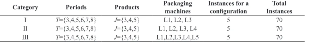
taking into account three categories of examples,

each containing 70 generated problem instances as shown in Table 2.

Initially, consider category I in a irst packaging coniguration, varying from 3 to 5 products, and 3 packaging machines (L1, L2, L3). The packaging capacity is 18,000 packages per hour, however without

a decreasing demand.

In this category, the tests with the data using Model Ia showed that the solution for the problem is infeasible when using only three machines with a capacity of

6,000 packages per hour each, as would be expected.

It is important to note that Model Ia assumes that every demand must be met without a delay. It must

be highlighted, once more, that the bottleneck of the production is the packaging machines, as we consider

that the liquid lavor preparation tank capacity always meets the packaging machine demands.

As the solutions were infeasible in category I, we considered the L4 machine in category II, adding

therefore a capacity of 7,500 packages per hour. However, it was still not possible to obtain feasible solutions with this coniguration for the 70 sample tests. Hence, in category III, we included the L5 machine, adding a capacity of 11,200 packages per

hour. In this category, the problem became feasible, meeting demands and providing optimal solutions within the imposed time limit.

Our results point to the fact that the factory expansion plan (i.e. adding one more machine) was

beneicial in order to obtain production schedules

that do not include any delays in meeting demands. The CPLEX solver solved all instances in category III, presenting optimal solutions within the time limit. This shows the potential of Model Ia to be used by the company on a daily basis. It is important to note that the computational time required to solve the model was less than one second, which means that these instances were easily solved by CPLEX.

4.3 Model Ib

The computer setting and the parameters used in this study are the same as the previous tests with Model Ia, as well as the random generator for the item demands. Owing to the fact that the Model Ia

instances were solved quickly, the test categories for

Model Ib were slightly different. In these new tests, we increased the number of items, surpassing 5. Furthermore, the time frame was increased to more than 8 periods per category, not exceeding a period

of 13 weeks, equivalent to a planning horizon of

3 months. Although this study aims to support production scheduling decisions at an operational level (short term decisions), and is not intended to propose a tool for midterm decisions, the number of products and periods was increased in these tests to study the behavior of Model Ib as the number of variables and constraints increase. When the time frame and the number of items go up, the number of constraints and variables are also increased.

The Model Ib tests included instances with time periods varying from 6 to 13, items varying from

5 to 10 and the possibility of using all 5 packaging

machines. For each possibility, 5 sample tests were

generated, making a total of 65 categories. Within

Table 2. Categories of examples used in Model Ia.

Category Periods Products Packaging

machines

Instances for a

coniguration InstancesTotal

I T={3,4,5,6,7,8} J={3,4,5} L1, L2, L3 5 70

II T={3,4,5,6,7,8} J={3,4,5} L1, L2, L3, L4 5 70

each problem category, most of the test instances were solved optimally within the time limit of one hour. Categories with time periods 11 and 13 were not included in the previous statement. The fact that the tests with such time frames (when considering 5 different items) were not easily solved reinforced the potential for the model´s practical use.

For every test sample for which the CPLEX

solver could not ind the optimal solution within the time limit, the Gap value was calculated by

( )

100 ( )

Gap= OF−IL OF , where OF is the objective function value of the best solution provided by the CPLEX solver and IL is the best lower bound as given by CPLEX in one hour time limit.

The tests were run with and without constraints (8), and only in 16 out of 65 instances, the solver solved

the model more quickly with the constraint active.

On average, the tests without constraints (8) were 45% faster. The solutions of the 130 tests, with and without these constraints, showed the same behavior.

The gaps were relatively low. For the sake of

comparison, this study was used for the 65 instances without constraints (8), as they were solved faster and optimally. Only two instances reached the maximum execution time and the biggest gap was 0.25%.

Table 3 shows the results of the tests using model Ib concerning the use of production capacity

and backlog in relation to demand, as well as the stock concerning the demand. In the ifth column of the

table, the percentage of capacity is shown occupied by the setup execution (%Setup), while (%Production) represents the percentage of the capacity used for the

production of items. %Backorder is the backorder

ratio related to the demand in the last period and

%Inventory is the ratio of the stock in the last period

and the demand in the last period.

Table 3 shows that the average use of the capacities

did not exceed 70%, although there is a signiicantly small backorder ratio. The highest usage of capacity

was 72% in category 2 for one instance. It can be observed that because of the set of constraints (6), minimum lot, it is less expensive to have a minimum

of delay that meets all the demand and stock at the

end of the planning horizon. These results will be compared with the results from Model II, based on the CLSP, in the next section.

4.4 Model II

In this section, we present a comparison between the test results obtained from Model II when using the problem instances shown in Table 3 of Section 4.2. The solutions achieved by Models Ib and II were similar when considering the objective function values, the utilized production capacities, the ratios between inventory and demand and the ratios between

backorder and demand. The comparison between the models’ performances is illustrated in Table 4. Note that the number of optimal solutions drawn from each model (Nº*) are shown, as well as the average gap and the average running time for each test category. The symbol (*) indicates that the solver CPLEX was able to solve all test samples optimally.

Both models presented feasible solutions for all test

samples. However, Model Ib obtained more optimal

solutions than Model II. When the solutions of Model Ib were not optimal, the gaps were less than 0.35%. On the other hand, solutions from Model II could be found within the time limit and they presented a gap of 3.87%.

In category 10, Model Ib presented optimal solutions for all instances. In the same category, Model II was

able to ind only two optimal solutions and they

presented an average gap of 1.80%. On average, Model II was solved three times slower than Model Ib. In general, both models yielded solutions of good

quality. However, when we take into account the

average time and the number of optimal solutions, the performance of Model Ib was better than Model II.

Table 3. Model Ib test results - Solution characteristics

|J| |T| Nº example. %Setup %Production %Backorder %Inventory

1 5 6 5 2.0 58.37 0.47 0

2 5 7 5 2.3 68.51 0.04 0

3 5 8 5 2.18 59.50 0.67 0

4 5 9 5 2.40 57.44 0.35 0

5 5 10 5 1.98 56.71 0.36 0

6 5 11 5 1.98 57.39 0.64 0

7 5 12 5 2.01 57.43 0.26 0

8 5 13 5 2.04 56.90 0.38 0

9 6 13 5 1.99 57.33 0.19 0

10 7 13 5 2.10 57.33 0.00 0

11 8 13 5 2.06 57.40 0.17 0

12 9 13 5 2.01 56.90 0.41 0

This was unexpected as Model Ib is less simple because it considers scheduling decisions based on

the GLSPPL, unlike Model II which is based on

the CLSP.

It is worth mentioning that Model II still requires a post-processing step to review the sizes of the obtained lots and ensure that the solution is feasible from the point of view of the minimum and maximum allowable lots. This post-processing step consists of simply dividing the big lot, xjmt, (if it exceeds the

maximum lot) by the number of performed setups, that is, zjmt, and therefore, obtaining smaller lots

(Lmax a_m). Model Ib does not need a post-processing step and since the resolution of the instances with it was faster and sometimes resulted in better quality solutions (within the time limit) than Model II, it is concluded (on the basis of the results of this study) that Model Ib is the most recommended one to deal with this problem.

The results obtained from Models Ia, Ib and II were shown to the factory production manager and to the production programmer. As we mentioned earlier, the objective functions of Models Ib and II prioritize minimization of the overall production costs,

such as inventory, setup and backorder. However, the

objective function suggested by the manager was the one presented in Model Ia.

The solutions from Model Ia were the best according to the production programmer, because they were closer to what was already done in the factory. In the case of Model 1a, the objective function

gives priority to maximizing the proit margin and

does not consider the costs, therefore its solutions

avoid idle time. However, the programmer stated

that, considering the solutions in Model Ia, these lots could be too small, and therefore it would be better not to produce these products during these periods.

Therefore, it might be better not to make these lot

sizes in such time frames. A simple alternative to

avoid this type of solution would be to revise the parameters of Model Ia related to the minimum lot size corresponding to

q

It should be noted that the models presented here were solved by the solver Cplex using the branch-and-cut method and requiring only a few seconds for these samples, which are as large as the ones we were given by the factory. On the other

hand, the production programmer takes at least

40 minutes to come up with a feasible production plan. Both the production manager and the production programmer found that the solutions produced by Models Ia and Ib are potentially good to be used in practice. Any adjustments to adapt the models to

the speciic operational conditions might be of use, especially to obtain a production plan of each week

of the company. Interesting future research would be to develop an effective validation of the models using them in the company on a daily basis to better evaluate the advantages and disadvantages of the production schedules generated by the models in comparison with the schedules used in the factory.

5 Concluding remarks

This paper presented optimization models based on mathematical programming and applied methods of solution to solve them in order to support the

process of taking decisions regarding production planning and scheduling of fruit juice drink lines. A case study was undertaken in a production line

of a typical company of this sector. The proposed

models used a theoretical framework for the lot

sizing problems and to schedule production lots,

which are well known and explored in the literature.

Considering the results obtained, it can be concluded that the presented models and the tested methods are potentially good to support short term production planning decisions in this industry, for example,

considering time frames of 8 or 9 weeks. We believe Table 4. Model performance comparison.

|J| |T| Nº example.

Nº* model Ib

Nº* model II

Gap GLSP(%)

Gap CLSP(%)

Time GLSP(s)

Time CLSP(s)

1 5 6 5 5 5 * * 23.99 11.04

2 5 7 5 5 5 * * 15.99 22.59

3 5 8 5 5 5 * * 29.51 49.92

4 5 9 5 5 5 * * 74.87 53.87

5 5 10 5 5 5 * * 113.60 299.06

6 5 11 5 4 5 0.05 * 731.96 267.21

7 5 12 5 5 5 * * 345.15 137.03

8 5 13 5 4 5 0.02 * 743.53 365.36

9 6 13 5 5 5 * * 30.59 212.42

10 7 13 5 5 2 * 1.80 66.74 3,150.72

11 8 13 5 5 3 * 0.11 72.44 1,095.52

12 9 13 5 5 5 * * 71.91 444.80

13 10 13 5 5 3 * 0.48 313.68 1,837.71

that these approaches can be adopted successfully in the company under consideration and also in other companies in this industry, as well as other industrial sectors whose processes are similar. It is important to notice that the criteria for optimizing the lot sizing and scheduling could be different when considering costs related to preparation, inventories and delays, time limits, and minimum and maximum lots size capacities, among other factors.

Interesting future research would be to develop a user-friendly version of Model Ia, so that the production programmer of the company could test and evaluate

the eficiency of its solutions on a daily basis. Having

such results available, it would be possible to develop an effective case study and proceed to validating this model in real life situations. In this case, it would be interesting to evaluate the performance of the model in production scheduling and rescheduling, using rolling planning horizon approaches. Another motivating line of research would be to investigate effective heuristic methods to solve Models Ia, Ib and II in situations where optimization software, based on branch-and-cut algorithms, such as the one of the CPLEX solver, were not capable of providing good solutions within acceptable computer times.

Acknowledgements

The authors would like to thank the two anonymous

reviewers for their useful comments and suggestions. This research was partially supported by CNPq and FAPESP, Brazil.

References

Almada-Lobo, B., Oliveira, J. F., & Carravilla, M. A. (2008). Production planning and scheduling in the glass container industry: A VNS approach. International Journal of Production Economics, 114(1), 363-375. http://dx.doi.org/10.1016/j.ijpe.2007.02.052.

Araujo, S. A., Arenales, M. N., & Clark, A. R. (2008). Lot sizing and furnace scheduling in small foundries. Computers & Operations Research, 35(3), 916-932. http://dx.doi.org/10.1016/j.cor.2006.05.010.

Associação Brasileira das Indústrias de Refrigerantes e de Bebidas não Alcoólicas – ABIR. (2010). Recuperado em 10 de fevereiro de 2010, de http://abir.org.br/ Buschkühl, L., Sahling, F., Helber, S., & Tempelmeier,

H. (2010). Dynamic capacitated lot-sizing problems: a classification and review of solution approaches. OR-Spektrum, 32(2), 231-261. http://dx.doi.org/10.1007/ s00291-008-0150-7.

Clark, A. R. (2003). Hybrid heuristics for planning lot setups and sizes. Computers & Industrial Engineering, 45(4), 545-562. http://dx.doi.org/10.1016/S0360-8352(03)00073-1.

Defalque, C. M., Rangel, S., & Ferreira, D. (2011). Usando o ATSP na modelagem do problema integrado de produção

de bebidas. TEMA - Tendências em Matemática Aplicada, 12(3). http://dx.doi.org/10.5540/tema.2011.012.03.0195. Diário Econômico. (2011). Recuperado em 10 fevereiro

de 2011, de http://www.diariodepernambuco.com. br/2011/03/01/economia3_0.asp

Drexl, A., & Kimms, A. (1997). Lot sizing and scheduling - survey and extensions. European Journal of Operational Research, 99(2), 221-235. http://dx.doi.org/10.1016/ S0377-2217(97)00030-1.

Ferreira, D., Clark, A., Almada-Lobo, B., & Morabito, R. (2012). Single-stage formulations for synchronised two-stage lot sizing and scheduling in soft drink production. International Journal of Production Economics, 136(2), 255-265. http://dx.doi.org/10.1016/j.ijpe.2011.11.028. Ferreira, D., Morabito, R., & Rangel, S. (2009). Solution

approaches for the soft drink integrated production lot sizing and scheduling problem. European Journal of Operational Research, 196(2), 697-706. http://dx.doi. org/10.1016/j.ejor.2008.03.035.

Ferreira, D., Morabito, R., & Rangel, S. (2010). Relax and fix heuristics to solve one-stage one-machine lot-scheduling models for small-scale soft drink plants. Computers & Operations Research, 37(4), 684-691. http://dx.doi.org/10.1016/j.cor.2009.06.007.

Fleischmann, B., & Meyr, H. (1997). The general lot sizing and scheduling problem. OR-Spektrum, 19(1), 11-21. http://dx.doi.org/10.1007/BF01539800.

Glock, C. H., Grosse, E. H., & Ries, J. M. (2014). The lot sizing problem: A tertiary study. International Journal of Production Economics, 155, 39-51. http://dx.doi. org/10.1016/j.ijpe.2013.12.009.

Jans, R., & Degraeve, Z. (2008). Modeling industrial lot sizing problems: a review. International Journal of Production Research, 46(6), 1619-1643. http://dx.doi. org/10.1080/00207540600902262.

Karimi, B., Fatemi Ghomi, S. M. T., & Wilson, J. M. (2003). The capacitated lot sizing problem: a review of models and algorithms. Omega, 31(5), 365-378. http://dx.doi. org/10.1016/S0305-0483(03)00059-8.

Kopanos, G. M., Puigjaner, L., & Georgiadis, M. C. (2010). Optimal Production Scheduling and Lot-Sizing in Dairy Plants: The Yogurt Production Line. Industrial & Engineering Chemistry Research, 49(2), 701-718. http://dx.doi.org/10.1021/ie901013k.

Leite, R. P. M. (2008). Um estudo sobre o problema de dimensionamento e sequenciamento da produção no setor de bebidas (Trabalho de Conclusão de Curso). Universidade Federal de São Carlos, São Carlos. Luche, J. R. D., Morabito, R., & Pureza, V. (2009). Combining

process selection and lot sizing models for production scheduling of electrofused grains. Asia-Paciic Journal of Operational Research, 26(3), 421-443. http://dx.doi. org/10.1142/S0217595909002286.

Annals of Operations Research, 150(1), 177-192. http:// dx.doi.org/10.1007/s10479-006-0157-x.

Meyr, H. (2002). Simultaneous lotsizing and scheduling on parallel machines. European Journal of Operational Research, 139(2), 277-292. http://dx.doi.org/10.1016/ S0377-2217(01)00373-3.

Pagliarussi, M. S. (2013). Contribuições para a otimização da programação de bebidas à base de frutas (Dissertação de Mestrado). Universidade Federal de São Carlos, São Carlos.

Pirillo, C. P., & Sabio, R. P. (2009). 100% suco: nem tudo é suco nas bebidas de frutas. Revista HortiFruti Brasil, 81, 6-7. Recuperado em 10 fevereiro de 2011, de http://www.cepea.esalq.usp.br/hfbrasil/edicoes/81/ mat_capa.pdf

Rangel, S., & Ferreira, D. (2003). Um modelo de dimensionamento de lotes aplicado à indústria de bebidas. TEMA – Tendências em Matemática Aplicada, 4(2), 237-246.

Santos, M. O., & Almada-Lobo, B. (2012). Integrated pulp and paper mill planning and scheduling. Computers & Industrial Engineering, 63(1), 1-12. http://dx.doi. org/10.1016/j.cie.2012.01.008.

Sistema de Controle de Produção de Bebidas – SICOBE. (2005). Recuperado em 10 fevereiro de 2011, de http://idg.receita.fazenda.gov.br/orientacao/tributaria/ regimes-e-controles-especiais/sistema-de-controle-de-producao-de-bebidas-2013-sicobe

Toledo, C. F. M., França, P. M., Morabito, R., & Kimms, A. (2007). Um modelo de otimização para o problema integrado de dimensionamento de lotes e programação

da produção em fábricas de refrigerantes. Pesquisa Operacional, 27(1), 155-186. http://dx.doi.org/10.1590/ S0101-74382007000100009.

Toledo, C. F. M., França, P. M., Morabito, R., & Kimms, A. (2009). Multi-population genetic algorithm to solve the synchronized and integrated two-level lot sizing and scheduling problem. International Journal of Production Research, 47(11), 3097-3119. http://dx.doi. org/10.1080/00207540701675833.

Toledo, C. F. M., Kimms, A., França, P. M., & Morabito, R. (2015). The synchronized and integrated two-level lot sizing and scheduling problem: evaluating the generalized mathematical model. Mathematical Problems in Engineering, 2015, 1-18. http://dx.doi. org/10.1155/2015/182781.

Toledo, C. F. M., Oliveira, L., Pereira, R. F., França, P. M., & Morabito, R. (2014). A genetic algorithm/mathematical programming approach to solve a two-level soft drink production problem. Computers & Operations Research, 48, 40-52. http://dx.doi.org/10.1016/j.cor.2014.02.012. Toso, E. A. V., Morabito, R., & Clark, A. R. (2009). Lot-Sizing and Sequencing Optimisation at an Animal-Feed Plant. Computers & Industrial Engineering, 57(3), 813-821. http://dx.doi.org/10.1016/j.cie.2009.02.011.