doi: 10.1590/0101-7438.2015.035.03.0539
METAHEURISTICS EVALUATION:
A PROPOSAL FOR A MULTICRITERIA METHODOLOGY*
Valdir Agustinho de Melo and Paulo Oswaldo Boaventura-Netto
**Received July 16, 2014 / Accepted September 3, 2015
ABSTRACT.In this work we propose a multicriteria evaluation scheme for heuristic algorithms based on the classic Condorcet ranking technique. Weights are associated to the ranking of an algorithm among a set being object of comparison. We used five criteria and a function on the set of natural numbers to create a ranking. The discussed comparison involves three well-known problems of combinatorial optimization – Traveling Salesperson Problem (TSP), Capacitated Vehicle Routing Problem (CVRP) and Quadratic As-signment Problem (QAP). The tested instances came from public libraries. Each algorithm was used with essentially the same structure, the same local search was applied and the initial solutions were similarly built. It is important to note that the work does not make proposals involving algorithms: the results for the three problems are shown only to illustrate the operation of the evaluation technique. Four metaheuristics – GRASP, Tabu Search, ILS and VNS – are therefore only used for the comparisons.
Keywords: comparison among heuristics, metaheuristics, TSP, CVRP, QAP.
1 INTRODUCTION
1.1 Heuristics evaluation in the literature
This work is dedicated to a proposal of a multicriteria evaluation scheme for heuristic algorithms, which we called the Weight Evaluation Method (WOM). It involves an application of the Con-dorcet ranking technique, presented in Item 1.2. The initial discussion of WOM is the object of Item 1.3. Sections 2 and 3 present, respectively, quick explanations on the three problems and the four metaheuristics used in the tests. The use of the evaluation technique is detailed in Sec-tion 4 with the aid of an example. SecSec-tion 5 presents the results of the comparison among the metaheuristics when used with the three problems. The conclusions are exposed in Section 6.
The use of metaheuristics to find good quality solutions for discrete optimization problems has the double advantage of working with algorithms based on models already known and the effi-ciency of the methods themselves. This is very important when dealing with problems that have
*A preliminary version of this work was presented at Euro XXV, Vilnius, July 2012. **Corresponding author.
an exponential number of feasible solutions. When there are many techniques available, it is clearly important to evaluate their efficiency with respect to a given problem. A number of direct evaluation techniques, both deterministic and probabilistic, is commonly used, such as in Aiex et al. [2, 3] where their observations lead to the hypothesis that the iteration processing times of the heuristics based on local searches, aiming at a result with a determined target, follow an exponential distribution. The use of instance collections, available in the Internet for many prob-lems, appears there and in a number of other works as an efficient way to evaluate metaheuristics and compare their efficiency when dealing with a variety of situations.
Tuning parameters of an algorithm for improved efficiency is also a work that benefits from a system of assessment. Averages of execution times and final solution values, with their standard deviations, are often used. The normal distribution is commonly considered on these occasions, an option which is criticized by Taillard et al. [23] as a hypothesis not always verified: for example, if there are many global optima, the distribution will have a truncated tail, since it is impossible to go beyond the optimum.
There are in the literature several techniques for this purpose: following this reference, the most common are:
1. When dealing with optimization, a set of problem instances is solved with a couple of methods that should be compared, by calculating mean and standard deviation (possibly also other measures such as median, minimum, maximum, etc.) of the values obtained in a series of algorithm rounds.
2. In the context of exact problem-solving, the computational effort required to obtain the best solution is measured, and its mean, standard deviation an so on, are calculated.
3. The maximum computational effort is fixed, as well as a goal to reach, by counting the number of times each method achieves the goal within the computational time allowed.
In practice, often the measures computed by the first and second techniques are very primitive and it is common to calculate only the averages, which are insufficient to assert a statistical advantage of a method of solution in relation to another.
1.2 The Condorcet technique
1.3 The Weight Evaluation Method (WOM)
In this method we begin with a Condorcet-type ranking matrix. We use weights associated to the ranking of the algorithms from a set being object of comparison with respect to instances of a given problem. In this work, we define five evaluation criteria (see Item 4.2 below) and we apply a function on the set of natural numbers to the ranking given by each criterion. The valuation is defined such that thebetter resultsare associated to thelesser criterion values.
In this work, we cross three combinatorial optimization problems – theTraveling Salesperson Problem(TSP), theCapacitated Vehicle Routing Problem(CVRP) and theQuadratic Assignment Problem(QAP) – against four different metaheuristics: theGreedy Randomized Adaptive Search Procedure (GRASP), theIterated Local Search (ILS), theTabu Search (TS) and the Variable Neighborhood Search (VNS). To do that, we took instance collections of each problem from public libraries and made ten independent runs with each one, using an execution time limit of 600 seconds. We looked for solutions with Optimal or Better-Known Values (OBKV), according to the more recent information available on the Internet.
The algorithms were programmed in C language and ran on a Linux platform. In order to al-low for a very basic comparison, each algorithm was used with essentially the same structure, the same local search was used in every case and the initial solutions were similarly built. The only differences are the specific characteristics of each problem: the problem constraints and the objective function calculation. We adopted this option owing to the number of improvements al-ready existing in the literature, since the paper objective is to use the problem-algorithm crossing to show the functioning of the method andnotto propose any algorithm improvement.
The use of a sort function facilitates the visualization of orders. The sum of the values obtained with each algorithm for each problem makes easier the comparison between the algorithms and their sensitivities to every problem. It also allows us to evaluate the in-the-whole performance of an algorithm.
2 TEST PROBLEMS USED IN THE STUDY
The problems used in this study and presented below are widely known by the scientific commu-nity and often used as benchmarks for the validation of new algorithms, owing to their algorith-mic complexity [8, 21].
2.1 Traveling Salesperson Problem (TSP)
2.2 Capacitated Vehicle Routing Problem (CVRP)
Since the work published by Dantzig & Ramser in 1959 [5], many papers related to the Vehicle Routing Problem (VRP) has been seen in the literature. Some studies show different variants, such as more than one deposit, a time limit of delivery, different types of vehicles, delivery and collection of products, among others. In this work we make use of its classical modeling, which is to meet a set of customers through a fleet of vehicles of the same capacity. Each vehicle comes from a deposit and the sum of the demands associated with each customer cannot exceed the vehicle capacity.
2.3 Quadratic Assignment Problem (QAP)
Consider the problem of allocating pairs of activities to pairs of locations, taking into account the costs of travel distances between locations and some flow units conveniently defined between activities. The Quadratic Assignment Problem (QAP), proposed by Koopmans & Beckmann [14], is the problem of finding a minimum cost allocation of activities to locations where costs are determined by the sum of the products distance-flow.
3 METAHEURISTICS USED IN THE STUDY
The implementations used here for the metaheuristics vary greatly in efficiency. This was deemed appropriate to facilitate the observation of how WOM works.
3.1 Tabu Search
The Tabu Search was introduced by Fred Glover [9, 10] for integer programming problems and more recently perfected by Taillard [22]. This metaheuristic is based on the establishment of restrictions that effectively guide a heuristic search in exploring the solution space, trying to avoid that the search returns to previously visited solutions. These restrictions work in different ways, such as excluding the search of certain alternatives, classifying them as temporarily banned or taboos, or modifying ratings and selection probabilities, designating them as aspiration criteria.
3.2 GRASP
GRASP – Greedy Randomized Adaptive Search Procedure – proposed by Feo & Resende [7] – can be seen as a metaheuristic which uses the good characteristics of the purely random al-gorithms and the purely greedy processes in the construction phase. It is a multistart iterative process in which each iteration consists of two phases: the construction phase, where a feasible solution is constructed, and the local search phase, where a local optimum is found in the vicinity of the initial solution and, if necessary, the update of the best solution found so far is made.
3.3 ILS
of initial solution, (b) disturbance, which generates new starting points for local search, (c) the acceptance criterion that decides from which solution the search will be continued, (d) the local search procedure is defined as the search space.
3.4 VNS
VNS – Variable Neighborhood Search – was proposed by Hansen & Mladenovic´ [11, 12]. It is based on a systematic neighborhood exchange associated with a random algorithm to determine starting points of local search. The basic VNS scheme is very simple and easy to implement. Unlike other metaheuristics based on local search methods, VNS does not follow a trajectory but explores incrementally more or less distant neighborhoods of the current solution, ranging from the current solution to the new, if and only if an improvement occurs. According to the authors, the advantage of using various neighborhoods is that the local optimum in relation to a neighborhood is not necessarily the same from others: thus, the search should continue in a way downward (or upward) until the solution current is a minimum (or maximum) location of all structures of the pre-selected neighborhoods.
4 DETAILS ON CONDORCET AND WOM TECHNIQUES
In this section we present in more detail the proposed performance criteria, the application of the Condorcet method and the use of its results to generate the indicators associated with WOM.
4.1 Performance criteria for the proposed versions
Following the already cited concern of Taillard et al. [23] about the dependency of heuristic efficiency on instance type, we built a multicriteria evaluation with five comparison criteria. The criteria definitions below are such that lower values represent better results.
a) Number of not-OBKV solutions obtained (nopt)
b) Average relative value distance (avd)
This is the average of the values(obtained value – OBKV)/OBKV, for those tests not reaching the OBKV, expressed in percentages.
c) Quality index (qual)
This is a tailor-made function used to express performance, whether the algorithm reaches the OBKV or not. We used:
I(nsol,err or)=n Sol N ot Ot m∗(Avg Err or%)+n Sol Ot m−1 (4.1)
As an example, let us consider that in 10 executions of an instance, 8 produced the OBKV and 2 presented an average error of 1.3%. The index value is thenI =0.125+(2×1.3)=2.725. If the error of those two instances were 21.6%, we would haveI =0.125+(2×21.6)=43.325. We can see that the index is sensitive to the presence of bad solutions and that its value decreases when the number of OBKV solutions grows.
d) Average execution time (exec)
This includes only the instances where OBKV was obtained before the maximum execution time (600 seconds).
e) Average stagnation time complement (stag)
This shows the average difference between the maximum execution time of 600 seconds and the time associated with the last improvement in the solution value before the algorithm stops by maximum time criterion. Whenever the algorithm gets the OBKV, this value is nullified. This criterion can be associated with an algorithm capacity to avoid sticking at local optima.
4.2 Some details on the Condorcet technique
As discussed in Item 1.2, the Condorcet technique is based on a pairwise evaluation, seeking to order pairs of results, looking for obtaining a measure for performance differences, as detailed in what follows.
Let W be a set ofw objects o1,o2, . . . ,ow and let us consider theirw! permutations. Each
permutation pk(1≤ k≤ w!)induces aclassification Ok, that is, an order relation in which the
objectoi is said to bebetteroreasier than oj according to the order Ok, ifoi precedesoj in
Ok(oi <oj). The pair(oi,oj)is said to show adiscrepancy betweenOp andOq if and only
if oi < oj in the orderOpandoj < oi in the order Oq. Thedistancebetween Op and Oq,
dist(Op,Oq), is defined as the number of discrepant pairs among theCw,2possible ones. We
can then define therelative errorofOpwith respect toOqas:
εpq=100∗dist(Op,Oq)/Cw,2 (4.2)
This technique can be used to compare the performance of a pair of algorithms with respect to a given instance. Let then|W| = wthe number of algorithms that will be compared with a total ofzevaluation criteria, whose values refer to a given instance, each criterion generating a possibly different order. Acriterion-algorithmtable is obtained for each instance, whereeach position containsthealgorithm numberand itscorresponding criterion value. In this table, the algorithm number in each entry corresponds to that of the corresponding column.
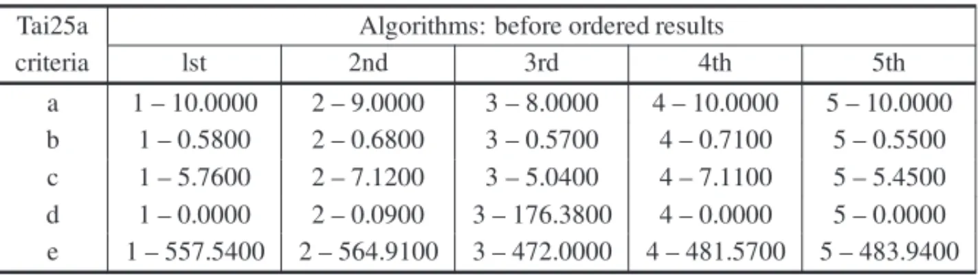
We exemplify the method with the QAP instance Tai25a, used among other QAP instances for testing five VNS variations, [16] (Table 1).
Table 1– Instance Tai25a – The matrix with the values obtained by the algorithms.
Tai25a Algorithms: before ordered results
criteria lst 2nd 3rd 4th 5th
a 1 – 10.0000 2 – 9.0000 3 – 8.0000 4 – 10.0000 5 – 10.0000 b 1 – 0.5800 2 – 0.6800 3 – 0.5700 4 – 0.7100 5 – 0.5500 c 1 – 5.7600 2 – 7.1200 3 – 5.0400 4 – 7.1100 5 – 5.4500 d 1 – 0.0000 2 – 0.0900 3 – 176.3800 4 – 0.0000 5 – 0.0000 e 1 – 557.5400 2 – 564.9100 3 – 472.0000 4 – 481.5700 5 – 483.9400
Table 2– Instance Tai25a – Criteria values in nondecreasing order.
Tai25a Algorithms: after ordered results
criteria lst 2nd 3rd 4th 5th
a 3 – 8.0000 2 – 9.0000 1 – 10.0000 4 – 10.0000 5 – 10.0000 b 5 – 0.5500 3 – 0.5700 1 – 0.5800 2 – 0.6800 4 – 0.7100 c 3 – 5.0400 5 – 5.4500 1 – 5.7600 4 – 7.1100 2 – 7.1200 d 1 – 0.0000 4 – 0.0000 5 – 0.0000 2 – 0.0900 3 – 176.3800 e 3 – 472.0000 4 – 481.5700 5 – 483.9400 1 – 557.5400 2 – 564.9100
In the next step, we examine each value pair along each line, considering the algorithms which produced the corresponding results. We represent the comparison result by a matrix where each column corresponds to a pair of algorithms and each entry value isk∈ {−1,0,+1}. The value choice fork is given by (+1;>); (−1, <); (0,=)(e.g., Criterion a gives the second posi-tion to Algorithm 2 (value 9.0000) and the fourth one to Algorithm 4 (value 10.0000), hence
(a,[2,4])= −1, while Criteriondgives the first position to Algorithm 1 and the second one to Algorithm 4 (both with value 0.0000); hence,(d,[1,4])=0).
Table 3– Instance Tai25a – The value pair comparison matrix.
Tai25a Algorithms
criteria [1,2] [1,3] [1,4] [1,5] [2,3] [2,4] [2,5] [3,4] [3,5] [4,5]
a 1 1 0 0 1 –1 –1 –1 –1 0
b –1 1 –1 1 1 –1 1 –1 1 1
c –1 1 –1 1 1 1 1 –1 –1 1
d –1 –1 0 0 –1 1 1 1 1 0
e –1 1 1 1 1 1 1 –1 –1 –1
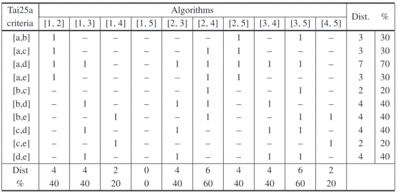
The last row and column of Table 4 are used for indicator evaluation. If all pairs have very high disagreements, for example, over 75%, a questioning about their validity will be convenient.
For this example of Tai25a instance, only the criteria pair[a,d]shows a higher disagreement (70%). The other pairs have better consistency, which indicates this criteria set as having good evaluation capacity for the algorithms applied to this instance. We can also look at the columns sum. It is interesting to observe that [1,5] column indicates no discrepancy, which is the same to say that Algorithms 1 and 5 are equivalent, according to all criteria utilized.
The Condorcet method proceeds by calculating the relative errors to be included in Eqn. 4.2 and preparing comparison tables based on those results. The number of comparisons will grow to O(w2)for each instance. The final evaluation would be done by inspection, since it becomes difficult to establish logical criteria which could be used for computational evaluation. Since the number of alternatives may be large, according to the value ofw, we consider the Condorcet technique as becoming impractical.
Table 4– Instance Tai25a – Comparison between pairs (by algorithms and by criteria).
Tai25a Algorithms
Dist. % criteria [1,2] [1,3] [1,4] [1,5] [2,3] [2,4] [2,5] [3,4] [3,5] [4,5]
[a,b] 1 – – – – – 1 – 1 – 3 30
[a,c] 1 – – – – 1 1 – – – 3 30
[a,d] 1 1 – – 1 1 1 1 1 – 7 70
[a,e] 1 – – – – 1 1 – – – 3 30
[b,c] – – – – – 1 – – 1 – 2 20
[b,d] – 1 – – 1 1 – 1 – – 4 40
[b,e] – – 1 – – 1 – – 1 1 4 40
[c,d] – 1 – – 1 – – 1 1 – 4 40
[c,e] – – 1 – – – – – – 1 2 20
[d,e] – 1 – – 1 – – 1 1 – 4 40
Dist 4 4 2 0 4 6 4 4 6 2
% 40 40 20 0 40 60 40 40 60 20
4.3 The Weight Ordering Method – WOM
The situation we have just described calls for some evaluation improvement. It led us to propose a Condorcet-like technique where the comparison can be easily made by calculation, the Weight Ordering Method (WOM). Here we have the advantage of automatically translate the results of the comparisons into numeric values. We do it with the aid of a function designed to beinjective for the considered value set: then, we can be sure it will condense in numbers the information provided by Table 4 above.
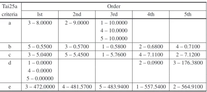
Table 5– WOM method – rearrangement of equal values for Tai25a.
Tai25a Order
criteria lst 2nd 3rd 4th 5th
a 3 – 8.0000 2 – 9.0000 1 – 10.0000 4 – 10.0000 5 – 10.0000
b 5 – 0.5500 3 – 0.5700 1 – 0.5800 2 – 0.6800 4 – 0.7100 c 3 – 5.0400 5 – 5.4500 1 – 5.7600 4 – 7.1100 2 – 7.1200
d 1 – 0.0000 2 – 0.0900 3 – 176.3800
4 – 0.0000 5 – 0.00000
e 3 – 472.0000 4 – 481.5700 5 – 483.9400 1 – 557.5400 2 – 564.9100
We do not consider the empty entries in the ordering (e.g., Line (d): Algorithm 2 in column 4 will besecondin order, not fourth; Algorithm 3 will bethird, not fifth).
With these data we are able to create anOi j – type matrix, similar to that of Condorcet method.
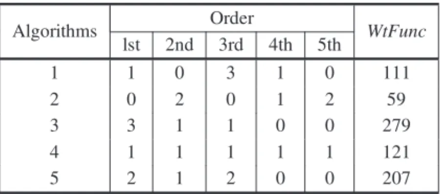
(Table 6), where each entry(i,j)contains the number of times Algorithmi appears in order j,for the whole criteria setapplied to a given instance. (e.g., Table 5 shows that Algorithm 1 obtained one first position (with Criterion d), three third positions (criteriaa, b, c) and one fourthposition (criterione)).
Table 6– WOM method – ordering matrix for Tai25a.
Algorithms Order
lst 2nd 3rd 4th 5th
1 1 0 3 1 0
2 0 2 0 1 2
3 3 1 1 0 0
4 1 1 1 1 1
5 2 1 2 0 0
To quantify the performance of each algorithm we use this matrix to associate with aweight functionover the obtained set of orders, where a first-rated algorithm receives a greater value than the second-rated one and so on. The suggested weight function (4.3) for a given algorithm considers the number w of algorithms, the order of the algorithm i for a given instance, an exponent basiskand the matrixO= [Oi j]of the instance, as follows:
W t Funci =
w
j=1
Oi j∗kw−j+1 (4.3)
It is crucial to observe that we are already working with an ordered set: since the function values reflect the ordering of the multicriteria evaluation for each algorithm, they correspond to the pairwise ordering used by Condorcet method, condensing its results into numeric values which indicate the algorithm performance order according to the proposed criteria.
Table 7 is Table 6 with a new column showingWtFuncvalues. We can see that the best global performance was that of Algorithm 3 (279) and the worst, that of Algorithm 2 (59).
Table 7– WOM method – final algorithm ordering for Tai25a.
Algorithms Order WtFunc
lst 2nd 3rd 4th 5th
1 1 0 3 1 0 111
2 0 2 0 1 2 59
3 3 1 1 0 0 279
4 1 1 1 1 1 121
5 2 1 2 0 0 207
It is important to mention that these results are consistent only within a given situation, since the orderings obtained in two different situations may not be consistent with one another and it may not be significant to add up their respective ratings.
5 COMPUTATIONAL RESOURCES AND RESULTS
For each problem, we used about 100 test instances, taken from their respective websites, [24] for TSP and CVRP, and [19] for QAP.
All algorithms departed with randomly generated initial solutions. We performed a set of ten executions for each instance, each one initialized with a new seed in order to ensure inde-pendence. The seeds were randomly selected from the list of prime numbers between 1 and 2,000,000, [6]. The tests were run on a computer with an Intel Core 2 Quad 2.4 GHz with 4 GB of RAM, under the Linux operating system,openSUSEdistribution.
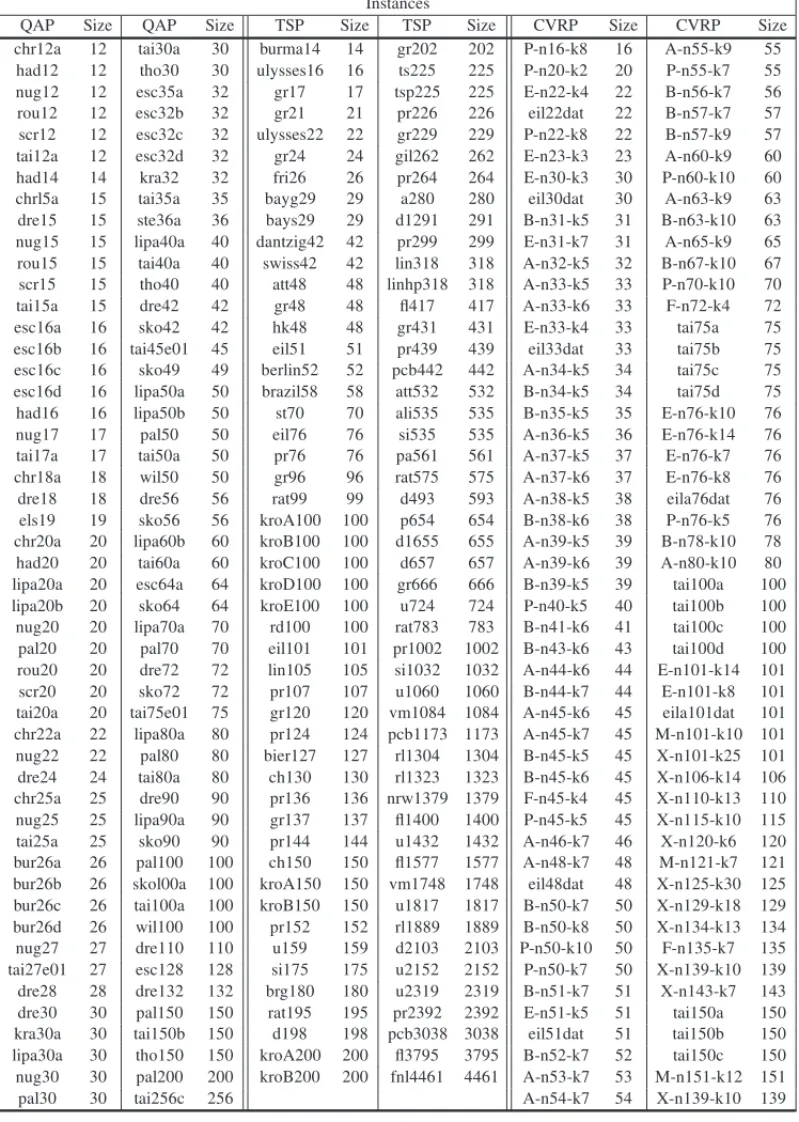
Table 8 contains the list of instances from the three problems, with the corresponding sizes.
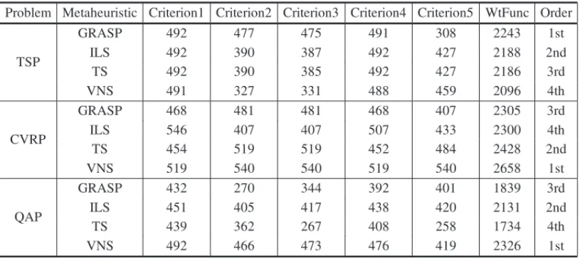
Table 9 shows the values of the weight function associated with the four algorithms, working on the problems used in the test. We can see that GRASP was the better technique both on TSP and on CVRP, while VNS worked more efficiently on QAP.
It may be noted that no algorithm was better than the others for the three problems. Although behavior differences should be expected between an algorithm-problem pair and another one, the results have also been influenced by our use of basic versions, which detailed descriptions can easily be found in the literature.
Table 8– Tested instances for QAP, TSP and CVRP. Instances
QAP Size QAP Size TSP Size TSP Size CVRP Size CVRP Size
chr12a 12 tai30a 30 burma14 14 gr202 202 P-n16-k8 16 A-n55-k9 55 had12 12 tho30 30 ulysses16 16 ts225 225 P-n20-k2 20 P-n55-k7 55 nug12 12 esc35a 32 gr17 17 tsp225 225 E-n22-k4 22 B-n56-k7 56 rou12 12 esc32b 32 gr21 21 pr226 226 eil22dat 22 B-n57-k7 57 scr12 12 esc32c 32 ulysses22 22 gr229 229 P-n22-k8 22 B-n57-k9 57 tai12a 12 esc32d 32 gr24 24 gil262 262 E-n23-k3 23 A-n60-k9 60 had14 14 kra32 32 fri26 26 pr264 264 E-n30-k3 30 P-n60-k10 60 chrl5a 15 tai35a 35 bayg29 29 a280 280 eil30dat 30 A-n63-k9 63 dre15 15 ste36a 36 bays29 29 d1291 291 B-n31-k5 31 B-n63-k10 63 nug15 15 lipa40a 40 dantzig42 42 pr299 299 E-n31-k7 31 A-n65-k9 65 rou15 15 tai40a 40 swiss42 42 lin318 318 A-n32-k5 32 B-n67-k10 67 scr15 15 tho40 40 att48 48 linhp318 318 A-n33-k5 33 P-n70-k10 70 tai15a 15 dre42 42 gr48 48 fl417 417 A-n33-k6 33 F-n72-k4 72 esc16a 16 sko42 42 hk48 48 gr431 431 E-n33-k4 33 tai75a 75 esc16b 16 tai45e01 45 eil51 51 pr439 439 eil33dat 33 tai75b 75 esc16c 16 sko49 49 berlin52 52 pcb442 442 A-n34-k5 34 tai75c 75 esc16d 16 lipa50a 50 brazil58 58 att532 532 B-n34-k5 34 tai75d 75 had16 16 lipa50b 50 st70 70 ali535 535 B-n35-k5 35 E-n76-k10 76 nug17 17 pal50 50 eil76 76 si535 535 A-n36-k5 36 E-n76-k14 76 tai17a 17 tai50a 50 pr76 76 pa561 561 A-n37-k5 37 E-n76-k7 76 chr18a 18 wil50 50 gr96 96 rat575 575 A-n37-k6 37 E-n76-k8 76 dre18 18 dre56 56 rat99 99 d493 593 A-n38-k5 38 eila76dat 76 els19 19 sko56 56 kroA100 100 p654 654 B-n38-k6 38 P-n76-k5 76 chr20a 20 lipa60b 60 kroB100 100 d1655 655 A-n39-k5 39 B-n78-k10 78 had20 20 tai60a 60 kroC100 100 d657 657 A-n39-k6 39 A-n80-k10 80 lipa20a 20 esc64a 64 kroD100 100 gr666 666 B-n39-k5 39 tai100a 100 lipa20b 20 sko64 64 kroE100 100 u724 724 P-n40-k5 40 tai100b 100 nug20 20 lipa70a 70 rd100 100 rat783 783 B-n41-k6 41 tai100c 100 pal20 20 pal70 70 eil101 101 pr1002 1002 B-n43-k6 43 tai100d 100 rou20 20 dre72 72 lin105 105 si1032 1032 A-n44-k6 44 E-n101-k14 101 scr20 20 sko72 72 pr107 107 u1060 1060 B-n44-k7 44 E-n101-k8 101 tai20a 20 tai75e01 75 gr120 120 vm1084 1084 A-n45-k6 45 eila101dat 101 chr22a 22 lipa80a 80 pr124 124 pcb1173 1173 A-n45-k7 45 M-n101-k10 101 nug22 22 pal80 80 bier127 127 rl1304 1304 B-n45-k5 45 X-n101-k25 101 dre24 24 tai80a 80 ch130 130 rl1323 1323 B-n45-k6 45 X-n106-k14 106 chr25a 25 dre90 90 pr136 136 nrw1379 1379 F-n45-k4 45 X-n110-k13 110 nug25 25 lipa90a 90 gr137 137 fl1400 1400 P-n45-k5 45 X-n115-k10 115 tai25a 25 sko90 90 pr144 144 u1432 1432 A-n46-k7 46 X-n120-k6 120 bur26a 26 pal100 100 ch150 150 fl1577 1577 A-n48-k7 48 M-n121-k7 121 bur26b 26 skol00a 100 kroA150 150 vm1748 1748 eil48dat 48 X-n125-k30 125 bur26c 26 tai100a 100 kroB150 150 u1817 1817 B-n50-k7 50 X-n129-k18 129 bur26d 26 wil100 100 pr152 152 rl1889 1889 B-n50-k8 50 X-n134-k13 134 nug27 27 dre110 110 u159 159 d2103 2103 P-n50-k10 50 F-n135-k7 135 tai27e01 27 esc128 128 si175 175 u2152 2152 P-n50-k7 50 X-n139-k10 139 dre28 28 dre132 132 brg180 180 u2319 2319 B-n51-k7 51 X-n143-k7 143 dre30 30 pal150 150 rat195 195 pr2392 2392 E-n51-k5 51 tai150a 150 kra30a 30 tai150b 150 d198 198 pcb3038 3038 eil51dat 51 tai150b 150 lipa30a 30 tho150 150 kroA200 200 fl3795 3795 B-n52-k7 52 tai150c 150 nug30 30 pal200 200 kroB200 200 fnl4461 4461 A-n53-k7 53 M-n151-k12 151
Table 9– Comparison among the four metaheuristics using WOM.
Problem Metaheuristic Criterion1 Criterion2 Criterion3 Criterion4 Criterion5 WtFunc Order
GRASP 492 477 475 491 308 2243 1st
TSP ILS 492 390 387 492 427 2188 2nd
TS 492 390 385 492 427 2186 3rd
VNS 491 327 331 488 459 2096 4th
GRASP 468 481 481 468 407 2305 3rd
CVRP ILS 546 407 407 507 433 2300 4th
TS 454 519 519 452 484 2428 2nd
VNS 519 540 540 519 540 2658 1st
GRASP 432 270 344 392 401 1839 3rd
QAP ILS 451 405 417 438 420 2131 2nd
TS 439 362 267 408 258 1734 4th
VNS 492 466 473 476 419 2326 1st
6 CONCLUSIONS
The WOM technique allows us to choose the level of detail in an algorithm performance study. For example, we can check performances by using an isolated instance or a set of instance classes, as in [16]. Comparison between different versions of the same algorithm can be made much more easily than by using the Condorcet method (whose output file increases with the square of the number of elements and is designed to give results by inspection), since the WOM gathers the evaluation results on a single parameter. It is also easily adaptable to an insertion, a replacement or a removal of a criterion or algorithm under study, allowing for faster scanning and analysis of their results.
Based on the Condorcet method, WOM shows very clearly both algorithm strengths and weak-nesses and also allows for an overall comparison in terms of performance ordering. We believe, even with this small example, that we can show its efficiency to make comparisons and sorting techniques by performance in the midst of a much larger number of alternatives.
We think WOM can be very useful in algorithm development, when a researcher has to deal with a number of different, but similar, algorithm versions, or with several sets of different parameter values for a given algorithm. As for the Condorcet method, the proposed criteria set can be changed or modified according to the research objective.
A comparison with the boxplot analysis (Appendix 1) shows most of its results comparable with those of WOM, CVRP being the less precise, TSP matching well and QAP fairly good.
REFERENCES
[2] AIEX RM, RESENDEMGC & RIBEIROCCC. 2002. Probability distribution of solution time in GRASP: an experimental investigation.Journal of Heuristics,8: 343–373.
[3] AIEXRM, RESENDEMGC & RIBEIROCCC. 2005.TTTPLOTS: a PERL program to create time-to-target plots.AT&T.
[4] BARBUTCCP. 1990. Automorphismes du permuto`edre et votes de Condorcet.Math. Inform. Sci. Hum., 28E,111: 73–82.
[5] DANTZIGGB & RAMSERJH. 1959. The truck dispatching problem.Management Science,6(1): 80-91. INFORMS.
[6] ESTANYCP. 2010.Prime numbers. Available in: http://pinux.info/primos/, Accessed April 2010.
[7] FEO TA & RESENDE MGC. 1995. Greedy randomized adaptive search procedures.Journal of Global Optimization,6: 109–133.
[8] GAREYMR & JOHNSONDS. 1979. Computers and Intractability: A Guide to the Theory of NP-Completeness. A Series of Books in the Mathematical Sciences. San Francisco, Calif. Victor Klee, ed.
[9] GLOVERF. 1989. Tabu search-Part I.ORSA Journal on Computing,1: 190–206. [10] GLOVERF. 1989. Tabu search-Part II.ORSA Journal on Computing,2: 4–32.
[11] HANSENP & MLADENOVIC´ N. 1997. Variable neighborhood search.Computers and Operations Research,24: 1097–1100.
[12] HANSENP & MLADENOVIC´ N. 2001. Developments of variable neighborhood search. Les Cahiers du GERAD, G-2001-24.
[13] HOLLANDJH. 1975. Adaptation in natural and artificial systems. University of Michigan Press, Ann Arbor.
[14] KOOPMANSTC & BECKMANNMJ. 1957. Assignment problems and the location of economic ac-tivities.Econometrica,25: 53–76.
[15] LOURENC¸OHR, MARTINOC & STUTZLE¨ T. 2003. Iterated local search. Glover F & Kochenberger GA (editors), Handbook of Metaheuristics, Chapter 11, p. 321–353. Kluwer Academic Publishers.
[16] MELOVA. 2010. QAP: Investigations on the VNS metaheuristic and on the use of the QAP variance on graph isomorphism problems (in Portuguese). D.Sc. Thesis. Program of Production Engineering, COPPE/UFRJ, Rio de Janeiro, Brasil.
[17] MENGERK. 1931. Bericht ¨uber ein mathematisches Kolloquium.Monatshefte f¨ur Mathematik und Physik,38: 17–18.
[18] MOREIRAAST. 2006. Hybrid GRASP-Tabu algorithms using the structure of Picard-Queyranne ma-trix for the QAP (in Portuguese). D.Sc. Thesis. Program of Production Engineering, COPPE/UFRJ, Rio de Janeiro, Brazil.
[19] QAPLIB HOMEPAGE. 2012. http://www.seas.upenn.edu/qaplib/ Accessed on: 12/10/12.
[20] R CORETEAM. 2015. R: A language and environment for statistical computing. R Foundation for Statistical Computing, Vienna, Austria. URL http://www.R-project.org/.
[22] TAILLARDE. 1991. Robust taboo search for the quadratic assignment problem.Parallel Computing,
17: 443–455.
[23] TAILLARDE, WAELTIP & ZUBERJ. 2008. Few statistical tests for proportions comparison. Euro-pean Journal of Operational Research,185: 1336–1350.
[24] TSPLIB HOMEPAGE. 2012. http://comopt.ifi.uni-heidelberg.de/software/TSPLIB95/ Accessed on: 12/10/2012.
APPENDIX 1: BOXPLOT ANALYSIS
Here we present the boxplot set for each problem, each graphic box corresponding to a criterion, where the plots correspond to the four algorithms, GRASP, ILS, TS and VNS, respectively.
In order to have a better painting foravdandqual, we reconfigured the values on a percentual basis, by using the maximum obtained value as a standard. The new avdandqualvalues are calculated as follows,
newavd =100∗(avd−O B K V)/max(avd)andnewqual=100∗qual/max(qual).
The stagnation timestagwas also put on a percentual basis.
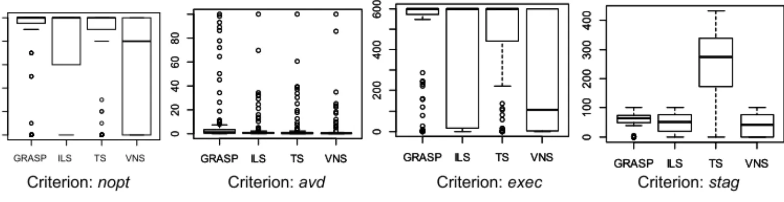
A discussion follows each set. We begin with the QAP boxplots (Fig. A1-1):
GRASP ILS TS VNS
0 1 00 2 00 300 400
GRASP ILS TS VNS
0 2 04 06 08 0
GRASP ILS TS VNS
0 2 00 4 00 6 00
GRASP ILS TS VNS
0 1 00 2 00 300 400
GRASP ILS TS VNS
0 2 04 06 08 0
GRASP ILS TS VNS
0 2 00 4 00 6 00
GRASP ILS TS VNS
02
46
81
0
Criterion: nopt Criterion: avd Criterion: exec Criterion: stag
Figure A1-1– Boxplot set for QAP.
For VNS, the number of not-OBKV solutions (nopt) covered the whole set of eleven possible values (from zero to 10). It seems then to be strongly instance-dependant, but all results are within the interquartile (IQ) zone. ILS ranks as second, TS as third and GRASP as fourth, but all with high median values.
The value average (avd) gave the lesser values for VNS among the four algorithms, ILS being second, GRASP third and TS fourth (only because of its outliers).
The quality index (qual) had no difference with respect toavd.
The stagnation time (stag) has the lesser median for VNS. TS presented the higher stagnation times and the higher median. GRASP was second and ILS, third. On the other hand, GRASP had the lesser value spread, followed by ILS, VNS, then TS.
We can say the boxplot comparison matches WOM results, VNS being easily the first, TS and ILS having near results and GRASP certainly worse.
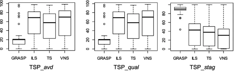
The TSP boxplots are in Figure A1-2 below.
GRASP ILS TS VNS
0 2 04 0 6 08 0 1 0 0
GRASP ILS TS VNS
0 2 0 4 0 60 80 100
GRASP ILS TS VNS
0 2 0 4 06 08 0
TSP_avd TSP_qual TSP_stag
GRASP ILS TS VNS
0 2 04 0 6 08 0 1 0 0
GRASP ILS TS VNS
0 2 0 4 0 60 80 100
GRASP ILS TS VNS
0 2 0 4 06 08 0
TSP_avd TSP_qual TSP_stag
Figure A1-2– Boxplot set for TSP.
The criterianopt andexec were not effective: since the TSP instances have real values, the algorithms spent all the allowed execution time of 600 seconds, within the ten executions for instance, trying to obtain better solutions within an interval of 1% fixed around the originally OBKV value given by the site, associated to the problem.
We can observe that GRASP produced lowavdandqual values. This behavior allows us to understand itsstagbehavior as a strong search for better values, most of them falling in the immediate neighborhood of the 1% region around OBKV. Since GRASP is a multistart method, along this process it would have less chance of sticking to local optima.
The same analysis, applied to the other three algorithms, points to less precision. We have to remember that, by the definition ofqual, it approachesavdwhen the number of successful trial goes to zero. Then the painting of the two criteria, here, is very similar and indicates that the stagnation time was consumed with worse solutions than those found by GRASP. The early stagnation also should mean the influence of local optima.
Considering this last point, VNS is the most susceptible and it presents also the higher values foravdand qual, showing the worst performance in this test. GRASP is evidently the most efficient and to decide between TS and ILS to be second and third it is convenient to consider the somewhat lesseravdandqualvalues of TS. It should then rank second and ILS third.
This result is the same obtained by the WOM technique (Table 7).
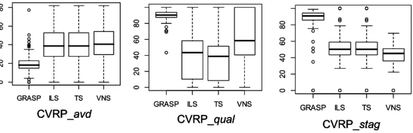
The CVRP boxplots are in Figure A1-3 below.
GRASP ILS TS VNS 0 2 04 0 6 08 0
GRASP ILS TS VNS
0 2 0 4 06 08 0
GRASP ILS TS VNS
0 2 04 0 6 08 0
CVRP_qual CVRP_stag
CVRP_avd
GRASP ILS TS VNS
0 2 04 0 6 08 0
GRASP ILS TS VNS
0 2 0 4 06 08 0
GRASP ILS TS VNS
0 2 04 0 6 08 0
CVRP_qual CVRP_stag
CVRP_avd CVRP_
qual CVRP_stag
CVRP_avd
Figure A1-3– Boxplot set for CVRP.
indicates the presence of greater distances related to the OBKV as final results. This is generally true, with the four algorithms.
By looking at the avdboxplot, GRASP could be considered the better technique, also in this case: but itsqualvalues show that its output is somewhat unstable. Then the interpretation of its highstagvalues – apparently similar to that of TSP – becomes less reliable.
The avd values for the other three algorithms are comparable, but when looking at thequal boxplot we observe an advantage of TS over ILS and VNS.
The stag values for ILS and TS are comparable, while VNS shows lesser values. This early stagnation seems, according toqual, to arrive at local optima.
It becomes difficult to classify GRASP in this case. ILS and TS are certainly in a middle position, and very close, while VNS should rank fourth. Here, the result is quite different from that shown by WOM (Table 7), which ranks VNS, TS, GRASP and ILS.