INTEGRADOS DE DISTRIBUIÇÃO E
MODELOS E ALGORITMOS PARA PROBLEMAS
INTEGRADOS DE DISTRIBUIÇÃO E
ROTEAMENTO
Tese apresentada ao Programa de Pós--Graduação em Ciência da Computação do Instituto de Ciências Exatas da Universi-dade Federal de Minas Gerais como req-uisito parcial para a obtenção do grau de Doutor em Ciência da Computação.
Orientador: Geraldo Robson Mateus
Coorientador: Alexandre Salles da Cunha
Belo Horizonte
MODELS AND ALGORITHMS FOR THE
INTEGRATED ROUTING AND DISTRIBUTION
PROBLEMS
Thesis presented to the Graduate Program in Computer Science of the Federal Univer-sity of Minas Gerais in partial fulfillment of the requirements for the degree of Doctor in Computer Science.
Advisor: Geraldo Robson Mateus
Co-advisor: Alexandre Salles da Cunha
Belo Horizonte
Santos, Fernando Afonso.
S237m Modelos e algoritmos para problemas integrados de distribuição e roteamento / Fernando Afonso Santos — Belo Horizonte, 2012.
xx, 116 f. : il. ; 29cm
Tese (doutorado) — Universidade Federal de Minas Gerais - Departamento de Ciência da Computação.
Orientador: Geraldo Robson Mateus Coorientador: Alexandre Salles da Cunha
1. Computação - Teses. 2. Otimização combinatória. I. Orientador. II. Coorientador. III. Título.
Since the Vehicle Routing Problem (VRP) was introduced by Dantzig and Ramser, it became one of the most studied problems in Combinatorial Optimization. Different solution approaches were proposed over the past decades to solve the VRP and its vari-ants. In this thesis, we discuss about two VRP variants, resulting from the integration of VRPs with distribution problems.
The first problem takes place by integrating the VRP with loading/unloading de-cisions in a Cross-Docking warehouse, which allows the consolidation of loads between their pickup and delivery. The problem of dealing with routing and distribution deci-sions at the Cross-Docking is named the Vehicle Routing Problem with Cross-Docking (VRPCD). We introduced two Integer Programming (IP) formulations for the VRPCD and respective branch-and-price (BP) algorithms to evaluate them. We also consider a slightly different approach for solving the VRPCD, where vehicles are allowed to bypass the Cross-Docking and loads eventually are not consolidated. We call this problem as the Pickup and Delivery Problem with Cross-Docking (PDPCD). We also introduced an IP model for the PDPCD and a BP algorithm to solve it.
The second problem we deal in this thesis arises in multi-echelon systems. The Two-Echelon Capacitated Vehicle Routing Problem (2E-CVRP) arises where loads must be shipped from a depot to customers passing through intermediate warehouses named satellites. Loads are shipped from the depot to satellites, where they are con-solidated before to be delivered to their respective customers. We propose an IP for-mulation for 2E-CVRP which holds an exponential number of variables. In addition, we introduce four families of valid inequalities for the problem. To solve such a formu-lation, including valid inequalities, we implement a Branch-and-cut-and-price (BCP) algorithm. Our computational results show that BCP algorithm evaluates stronger lower and upper bounds than previous algorithms for 2E-CVRP and also provides new optimality certificates for different instances of the literature.
Palavras-chave: Vehicle Routing Problems, Distribution Problems, Column Genera-tion, Branch-and-price, Cutting planes.
Após ter sido introduzido por Dantzig and Ramser, o Problema de Roteamento de Veículos (PRV) se tornou um dos problemas mais estudados em Otimização Combi-natória. Diferentes estratégias de solução foram propostas ao longo do tempo para solucionar o PRV e suas variações. Nesta tese, são discutidos dois problemas resul-tantes da integração do PRV com problemas de distribuição de mercadorias.
O primeiro problema a ser discutido surge da integração do PRV com decisões sobre carga/descarga de mercadorias em um Cross-Docking, que é um armazém que permite armazenamento de curta duração e a consolidação das cargas entre sua co-leta e a entrega. O problema resultante desta integração é denominado Problema de Roteamento de Veículos com Cross-Docking (PRVCD). São apresentados dois mode-los de programação inteira para o PRVCD e respectivos algoritmos Branch-and-Price
(BP) para solucionar tais modelos. Será discutida também uma abordagem alterna-tiva aos modelos tradicionais do PRVCD, na qual os veículos podem evitar passar pelo Cross-Docking na coleta/engrega de cargas, sem consolidá-las. Denomina-se esta nova abordagem de Problema de Coleta e Entrega comCross-Docking (PCECD). Uma formulação matemática e um novo algoritmo BP são introduzidos para solucionar o PCECD.
O segundo problema tratado surge dos sistemasmulti-elos. O Problema de Rotea-mento de Veículos Capacitado com 2 Elos (PRVC-2E) se caracteriza por definir o fluxo de cargas entre o depósito e seus consumidores finais, usando armazéns intermediários denominados satélites. Estes armazéns são responsáveis por integrar o primeiroelo, que contém o depósito, com o segundoelo, aonde estão dispostos os consumidores. Além do mais, as mercadorias podem ser consolidadas nos satélites a fim de minimizar os custos de entrega. São apresentados um modelo matemático para o PRVC-2E, que possui um número exponencial de variáveis, além de quatro famílias de desigualdades válidas para fortalecê-lo. A solução deste modelo, incluindo a separação das desigualdades válidas, é feita por um algoritmo Branch-and-cut-and-price (BCP). Os resultados obtidos pelo BCP mostram que o seu desempenho domina o de outros algoritmos propostos para o
Palavras-chave: Problemas de Roteamento de Veículos, Problemas de Distribuição, Geração de Colunas, Branch-and-price, Planos de corte.
1.1 Solution example for a VRP with 10 customers using 3vehicles. . . 2
2.1 An example of a VRPCD solution concerning 5 products and 2vehicles. . 24
2.2 Differences between possible solutions for VRPCD and PDPCD, with K = 3, n= 7. In the figures, k1, k2 and k3 denote routes. . . 27
2.3 Example of solution for the 2E-VRP . . . 30
3.1 Modifications on the graph to solve the pricing problem . . . 44
3.2 How path-relinking helps on the intensification of solutions of GRASP heuristic . . . 53
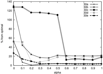
3.3 Evaluation of parameter α on heuristic behaviour . . . 54
3.1 Performance of the GRASP heuristic according to the number of iterations 53
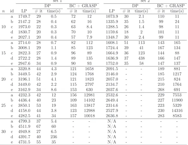
3.2 Performance of BP#2 for different pricing approaches for instances of sets 1 and 2 . . . 55
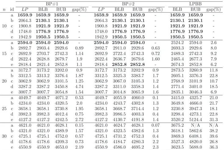
3.3 Computational results for set 1 neglecting loading/unloading costs at the CD (ci = 0,∀pi ∈P) . . . 57
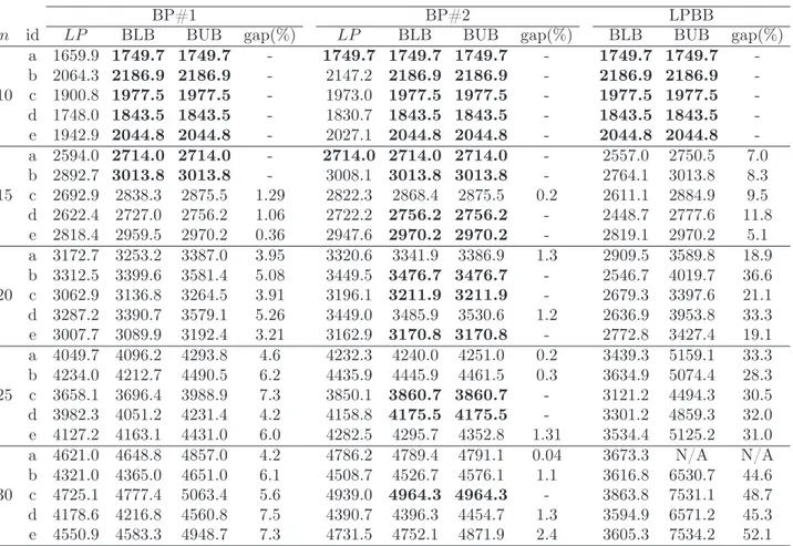
3.4 Computational results concerning loading/unloading costs asci = 20, ∀pi ∈
P for instances of set 1 . . . 58
3.5 Computational results concerning loading/unloading costs asci = 40, ∀pi ∈
P for instances of set 1 . . . 59
3.6 Computational results for instances with extended capacity (set 2). Load-ing/unloading costs at CD are neglected (ci = 0,∀pi ∈P) . . . 60
3.7 Solving instances of set 2 for loading/unloading costs as ci = 20, ∀pi ∈P . 61
3.8 Solving instances of set 2 for loading/unloading costs as ci = 40, ∀pi ∈P . 62
4.1 Comparing Branch-and-price algorithms for PDPCD and VRPCD on solv-ing instances of set 1: {ci = 0 :i= 1, . . . , n} . . . 71
4.2 Comparing Branch-and-price algorithms for PDPCD and VRPCD on solv-ing instances of set 1: {ci = 20 :i= 1, . . . , n} . . . 72
4.3 Comparing Branch-and-price algorithms for PDPCD and VRPCD on solv-ing instances of set 1: {ci = 40 :i= 1, . . . , n} . . . 73
4.4 Comparing Branch-and-price algorithms for PDPCD and VRPCD on solv-ing instances of set 2: {ci = 20 :i= 1, . . . , n} . . . 74
4.5 PDPCD - VF 6=S∪C -{ci = 40 :i= 1, . . . , n} . . . 75
5.1 Comparison of Linear Programming lower bounds and respective CPU times for Two-Echelon Capacitated Vehicle Routing Problem (2E-CVRP) - in-stances in sets 2 and 4. . . 93
5.3 Comparison of BCP, BP, BC-PER and BC-JEP - set 2. . . 96
5.4 Comparison of BCP, BP, BC-PER and BC-JEP - set 3. . . 96
5.5 Comparison of BCP, BP and BC-PER - set 4. . . 97
5.6 Aggregate results for BCP, BC-PER and BC-JEP. . . 98
5.7 Comparison of BCP, BP and BC-JEP - set 4. . . 100
Abstract xi
List of Figures xv
List of Tables xvii
1 Introduction 1
1.1 Objectives . . . 4
1.2 Main Contributions . . . 5
1.3 Thesis Outline . . . 6
2 Background and Literature Review 9
2.1 The Classical Vehicle Routing Problem . . . 9
2.1.1 The Vehicle Routing Problem with Backhauls . . . 14
2.1.2 The Vehicle Routing Problem with Time Windows . . . 16
2.1.3 The Vehicle Routing Problem with Pickup and Delivery . . . . 18
2.2 The Vehicle Routing Problem with Cross-Docking . . . 21
2.3 The Pickup and Delivery Problem with Cross-Docking . . . 26
2.4 The Two-Echelon Capacitated Vehicle Routing Problem . . . 27
3 Branch-and-price algorithms for the Vehicle Routing Problem with
Cross-Docking 35
3.1 Problem definition . . . 35
3.2 Branch-and-price Algorithm #1 . . . 36
3.2.1 Integer Programming Formulation . . . 36
3.2.2 Solving the Linear Programming relaxation by Column Generation 38
3.2.3 Column Generation Subproblem . . . 38
3.2.4 Algorithm’s Implementation Details . . . 39
3.3 Branch-and-price Algorithm #2 . . . 41
3.3.3 Column Generation Subproblem . . . 44
3.3.4 Algorithm’s Implementation Details . . . 50
3.4 Computational Experiments . . . 51
3.5 Concluding Remarks . . . 61
4 A Branch-and-price algorithm for the Pickup and Delivery Problem with Cross-Docking 63 4.1 Integer Programming Formulation . . . 63
4.2 Solving the Linear Programming relaxation by Column Generation . . 66
4.2.1 Column Generation Subproblems . . . 67
4.3 Further implementation details . . . 69
4.4 Computational Experiments . . . 70
4.5 Concluding Remarks . . . 75
5 A Branch-and-cut-and-price algorithm for the Two-Echelon Capac-itated Vehicle Routing Problem 77 5.1 Integer Programming Reformulations . . . 78
5.1.1 A reformulation that relies on routes that satisfy the elementarity condition . . . 79
5.1.2 A reformulation based on q-routes . . . 82
5.1.3 Valid Inequalities . . . 83
5.2 Branch-and-cut-and-price algorithm . . . 86
5.2.1 Evaluating the LP(F2) Bounds by Column Generation . . . 86
5.2.2 Strengthening the LP(F2) bounds with cutting planes . . . 87
5.2.3 Branching rules . . . 89
5.2.4 Further implementation details . . . 89
5.3 Computational Experiments . . . 90
5.3.1 Test instances . . . 90
5.3.2 Computational results . . . 91
5.4 Concluding Remarks . . . 98
6 Final Remarks 101
Bibliography 105
Introduction
Over the years, Operations Research tools have contributed significantly to reduce costs involved in the transportation of goods in logistic systems and to a better use of existing transportation infra-structure. Probably one of the first contributions in this domain is due toDantzig and Ramser [1959]. In that reference, a model and a solution procedure were given to solve the problem of routing vehicles to gas stations, from a central gasoline depot. Since that work, the term Vehicle Routing Problem (VRP) became used to represent a whole class of problems that involve routing vehicles from a central depot, in order to deliver (collect) goods to (from) customers (suppliers).
During the last fifty years or so, a huge growth on the number of different VRPs tackled both by the research community and by practitioners was noticed (seeLaporte
[2009] for an updated survey). Most of them incorporate operational constraints ini-tially ignored by the first VRPs studied.
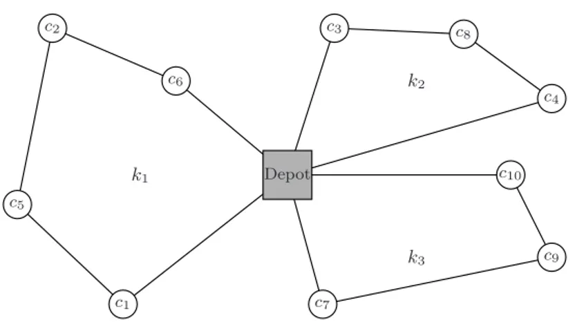
In Figure 1.1 we depict a solution for a VRP containing 3 vehicles and 10 cus-tomers. Each vehicle must leave the depot to visit a set of customers and return to the depot at end of the route. Each customer has a given demand and must be visited only once to be satisfied. In the figure, vehicles and customers are labeled as k1, . . . , k3
and c1, . . . , c10, respectively.
The VRP belongs to the class of NP-Hard problems, since the Traveling Salesman Problem (TSP) can be reduced to a VRP with a single uncapacitated vehicle. The need for better solutions for VRP and its variants motivated the development of an impressive number of exact and heuristic algorithms over the past decades. As the computational power available increased and the solution techniques improved, more real world applications have significantly shown to benefit from such developments. As a consequence, practitioners and researchers started to include more sophisticated constraints on VRPs aiming to solve real instances cases. Such modifications usually
Depot
c1
c2 c3
c4
c5
c6
c7
c8
c9
c10 k1
k2
k3
Figure 1.1: Solution example for a VRP with 10customers using 3vehicles.
lead to VRPs extensions for which to find optimal solutions become more complex, due to the increasing on the number of rules and constraints to tackle.
The recent advances in distribution systems have also motivated novel studies on VRPs. Logistics companies are extending the capabilities of warehouses for not only to store loads, but also allowing them to organize loads in order to improve their distribution along the logistic system. An example of such advances is the Cross-Docking warehouse [Apte and Viswanathan, 2000].
Cross-Docking (CD) is a warehouse proposed for helping in the transportation of loads without long-term inventory. Items delivered to a CD by inbound vehicles are immediately sorted out, reorganized based on customer demands and loaded into outbound vehicles for delivery, without the items being actually held in inventory at the warehouse. If any item is held in storage, it is usually for a brief period of time that is generally less than 24 hours [Yu and Egbelu, 2008].
The integration of VRPs with loads organization at CDs arises novel optimization problems. On the one hand, including scheduling decisions of loads organization at the CD, we enlarge the solutions space of problems. On the other hand, additional constraints must be introduced to ensure feasible solutions, defining more complex and challenging problems. The problem resulting from the integration of routing decisions on VRPs with loads organization at CDs is named Vehicle Routing Problem with Cross-Docking (VRPCD) [Lee et al., 2006].
from/to vehicles, and eventually optimizing their delivery. As VRPs, different variants of VRPCD can be considered, according to their characteristics. One can, for example, impose time windows constraints on suppliers and customers to ensure them to be served by vehicles in a proper interval or can either add additional costs to be incurred when loads change from/to vehicles at the CD.
The definition of VRPCD imposes that a given load must be collected at its supplier and stop at the CD for consolidation before to be delivered to their respective customer. Such a constraint may become solutions more expensive. For that reason, we propose here to allow loads to be delivered bypassing the CD, whenever such an operation reduce costs. To that end, we introduce pickup and delivery routes on the VRPCD. Vehicles implementing such routes are responsible for collecting a set of loads and delivering them immediately later, without stopping at the CD. As a result of such a modification, we state a novel optimization problem named the Pickup and Delivery Problem with Cross-Docking (PDPCD).
Another warehousing strategy frequently used in distribution systems is found in multi-echelon systems, on which echelons are linked using warehouses named satellites. Loads from inbound vehicles of a given echelon are delivered to a satellite, which also allows loads to be organized before to be loaded into outbound vehicles and shipped to the another echelon. Satellites are similar to CDs. However, loads are obligated to change from vehicles on satellites, while the loads changing is not compulsory at the CD and occurs only whether it optimizes the delivery.
Different combinatorial optimization problems may arise by integrating VRPs and organization of loads at satellites. The most recent problem dealing with VRP and loads scheduling at satellites is the Two-Echelon Capacitated Vehicle Routing Problem (2E-CVRP) [Perboli et al., 2008b]. The 2E-CVRP is the basic version of multi-echelon systems, since only two echelons are considered. On the 2E-CVRP a given load is available on the depot and must be shipped to customers using the satellites as intermediate depots. The routing is partitioned into level 1, where trucks are in charge of shipping loads from the depot to satellites and level 2, where small vehicles deliver the loads from the satellites to customers. After level 1 routing takes place, the loads are unloaded from trucks and organized into small vehicles to follow in level 2 routing. Therefore, the 2E-CVRP consists of assigning routes for vehicles on level 1 and level 2 for shipping loads from the depot to customers, as well as to define the organization of loads at satellites.
Moin and Salhi, 2007] is a well-known approach that integrates VRP and the inven-tory control problem. Solutions for IRPs consist of finding routes for vehicles to supply customers’ demands in a given planning horizon in order to minimize inventory and routing costs. Production planning problems and VRPs were also attacked together by different authors [Mak and Wong,1995;Fumero and Vercellis,1999;Yung et al.,2006;
Lejeune and Ruszczynski, 2007]. Their solutions concern routes for vehicles satisfying constraints on lot sizing and input/output of materials, commonly found in supply chains.
Even though VRPs may be integrated with other logistics facilities, we focus on this thesis our research on the VRPCD, PDPCD and 2E-CVRP. Such problems were considered because they integrate routing decisions with loads organization at warehouses. Moreover, they are recent in the literature. Therefore, studies on VR-PCD, PDPCD and 2E-CVRP can contribute with the continuous development of this promising area.
1.1
Objectives
Cross-Docking warehouses are widely used by global market companies like Toyota [Ohlmann et al., 2008], UPS [Forger, 1995] and Wal Mart [Gue, 2001]. However, the VRPCD literature has a small number of contributions [Lee et al., 2006; Wen et al.,
2009; Musa et al., 2010; Liao et al., 2010; Tarantilis, 2012]. In addition, to the best of our knowledge, no exact solution approaches were reported for neither VRPCD or PDPCD.
Similarly to VRPCD and PDPCD, the 2E-CVRP is a quite recent problem in the literature. Although multi-echelon systems and their related problems are well known in the literature, the first to propose models and algorithms to integrate the consolida-tion decisions on satellites with routing decision wasPerboli et al.[2008b]. After that, a few papers reported works on 2E-CVRP [Perboli and Tadei,2010;Perboli et al.,2011;
Crainic et al.,2011], but only one exact approach was proposed with a branch-and-cut algorithm.
beyond and also investigate families of valid inequalities in a branch-and-cut-and-price framework.
1.2
Main Contributions
We are going to report along this thesis some contributions concerning integer pro-gramming modeling and solutions for VRPCD, PDPCD and 2E-CVRP. The major contributions are:
• Two Integer Programming Formulations for the VRPCD and associated branch-and-price algorithms for solving such formulations;
• A deeper study on algorithms for solving the resulting column generation sub-problems. For instance, we implemented Dynamic Programming, Branch-and-cut and Heuristic algorithms for solving pricing problems;
• An Integer Programming Formulation and a branch-and-price algorithm to solve the PDPCD;
• An Integer Programming Formulation and valid inequalities are also proposed for the 2E-CVRP. A resulting branch-and-cut-and-price is also implemented to solve such formulation. Promising results are reported, including new optimality certificates for several instances of the literature.
In addition, we also contribute with scientific papers that have already been published (or accepted for publication):
• Santos F. A., da Cunha A. S., Mateus G. R., “Modelos de otimização para o Problema de Roteamento de Veculos comCross-Docking”, Simpósio Brasileiro de Pesquisa Operacional (SBPO), 2010 (in portuguese) [Santos et al.,2010]
• Santos F. A., da Cunha A. S., Mateus G. R., “Um Algoritmo Branch-and-price para o Problema de Roteamento de Veículos com Cross-Docking para Frotas Heterogêneas”, Simpósio Brasileiro de Pesquisa Operacional (SBPO), 2011 (in portuguese) [Santos et al.,2011a]
• Santos F. A., da Cunha A. S., Mateus G. R., “A novel column generation algo-rithm for the Vehicle Routing Problem with Cross-Docking”, International Net-work Optimization Conference (INOC), 2011 [Santos et al., 2011b]
• Santos F. A., da Cunha A. S., Mateus G. R., “Branch-and-Price Algorithms for the Two-Echelon Capacitated Vehicle Routing Problem”, Optimization Letters, 2012 [Santos et al., 2012a]
• Santos F. A., da Cunha A. S., Mateus G. R., “The Pickup and Delivery Problem with Cross-Docking”, Computers and Operations Research, 2012 [Santos et al.,
2012b]
1.3
Thesis Outline
On chapter 2 we discuss the background and related works associated with this thesis. We start introducing the classical VRP and some of its common variants: the VRP with Backhauls, the VRP with Time-Windows and the VRP with Pickup and Deliv-ery. Then, we formalize the VRPCD, the PDPCD and the 2E-CVRP and present a literature review with the most relevant contributions for each problem.
Those models and algorithms used to solve the VRPCD are introduced on chap-ter 3. We propose three integer programming models for solving the VRPCD: one based on network flow formulation and the two others based on set partitioning formu-lation, leading to models with an exponential number of variables. We implemented branch-and-price algorithms to solve the set partitioning based models. The algorithm implementation details, including different approaches for solving the pricing problems are also discussed on chapter 3, where we also present the computational experience of solving the VRPCD using the three proposed models.
We propose on chapter 4 a set partitioning based formulation for the PDPCD and also implemented a branch-and-price algorithm to solve it. Modeling and algorithm implementation details as well as further computational results for the PDPCD are also discussed on this chapter.
Background and Literature Review
The VRP is one of the most studied combinatorial optimization problems [Laporte,
2009;Toth and Vigo,2002b]. As increased the computational resources over the years, allowing powerful software-based engines to solve VRPs, as became complex the prob-lems, dealing with even more sophisticated real-world constraints. As a consequence of such a development, different VRP variants were proposed, including particular constraints from the real-world applications.
Recently, authors have proposed to integrate VRPs with logistics and distribution problems, leading to even more complex problems. In particular, the Vehicle Rout-ing Problem with Cross-DockRout-ing (VRPCD), the Pickup and Delivery Problem with Cross-Docking (PDPCD) and the Two-Echelon Capacitated Vehicle Routing Problem (2E-CVRP) were proposed to deal with routing decisions integrated with consolidation of loads in specific warehouses, respectively named Cross-Docking and Satellites. Con-solidation of loads is a modern trend in distribution systems, allowing loads to change from/to vehicles in order to satisfy routing constraints and minimizing costs.
In this chapter we discuss the classical VRP and its most common variants on section2.1, including a literature review on the most relevant research conducted in this area. On sections 2.2, 2.3 and 2.4 we formalize the problems dealt in this thesis: the VRPCD, the PDPCD and the 2E-CVRP, respectively. A literature review concerning such problems is also provided on each section.
2.1
The Classical Vehicle Routing Problem
In this section we are going to introduce some basic definitions about VRP and its most common variants. We also introduce integer programming models and a literature review on the most effective solution methods for each problem. For further reading
on VRP and variants we refer toToth and Vigo [2002b].
LetG= (V, A)be a directed graph where V ={0,1, . . . , n} represents the set of vertices and A={(i, j) :i, j ∈V;i6=j} denotes the set of arcs ofG. Vertices 1, . . . , n
correspond to the customers of the network, whereas vertex 0 identifies the depot (or warehouse). For each arc (i, j) ∈A we associate a nonnegative cost cij to denote the
cost to travel from vertex i to vertex j. Assume we are given a set K, containing K
vehicles, in charge to leave the depot for visiting customers and return back to depot at the end of the route. The VRP consists of assigningK routes, one for each vehicle ofK, for spanning all customers ofG, minimizing the traveling costs, given by the sum of arcs costs traversed by vehicles.
Further on the above definition, generally authors include capacity constraints in the VRP, leading to the Capacitated VRP (CVPR). In the CVRP, we assume that a nonnegative demand qi is assigned to each customer of G and consider a capacity
limitQk for each vehiclek ∈ K. Whether vehicles of setKhold the same capacity, the
problem is called homogeneous and we simplify the capacity limit to Q, otherwise we call it as heterogeneous CVRP. Along this thesis, we assume homogeneous problems as default. We also make use of both terms the VRP and the CVRP to refer to the Capacitated VRP. Furthermore, we interchangeably use the terms loads, goods, products and demands as well as vehicles and routes.
Although we stated above that exactlyKvehicles must be used in VRP solutions, is also possible to impose that feasible solutions use at most K vehicles. In addition, different objective functions could also be considered, for example, to minimize the number of vehicles used to meet the customers requirements, instead of minimizing the routing costs. All of these approaches are well-known in the literature and their use depend of the costs involved. In this thesis we deal only with the minimization of routing costs.
After introduced by Dantzig and Ramser [1959], an impressive number of algo-rithms were proposed to solve the VRP. A distinguished approach was proposed by
intersection of two polytopes, one associated with a Lagrangean relaxation, the other defined by bound, degree and capacity constraints, leading to a problem with an ex-ponential number of variables and constraints. The authors are able to solve instances of the literature with up to 135 customers. We refer to Toth and Vigo [2002a] for a survey on exact algorithms for the CVRP.
In the following we present a linear integer programming formulation for the CVRP extracted from Toth and Vigo [2002b]. The model is a two-index flow formu-lation that makes use of O(n2) binary decision variables x
ij indicating whether arc
(i, j)∈A is traversed in the solution or not, assuming respectively values 1 or0.
min X
(i,j)∈A
xijcij (2.1)
X j∈V
x0j =K (2.2)
X i∈V
xi0 =K (2.3)
X j∈V
xij = 1 ∀i∈V \ {0} (2.4)
X j∈V
xji = 1 ∀i∈V \ {0} (2.5)
X i /∈S
X j∈S
xij ≥π(S) S⊆V \ {0}, S 6=∅ (2.6)
xij ∈ {0,1} ∀(i, j)∈A (2.7)
The objective function (2.1) minimizes the piecewise costs of the traversed arcs in the solution. Constraints (2.2) and (2.3) impose that exactly K vehicles are used in the solution for visiting customers, while constraints (2.4) and (2.5) are respectively the outdegree and indegree constraints and are proposed to ensure that each customer is served exactly once in the solution.
Constraints (2.6) are the so-called capacity-cutset constraints. They are used to guarantee both connectivity and capacity constraint feasibility on solutions. The parameter π(S)define the minimum number of vehicles needed to satisfy the demands of vertices of the set S. One can solve a bin-packing problem to evaluate π(S) or alternatively can use the valid lower bound l
P i∈Sqi
Q m
It is easy to see that model (2.1)-(2.7) has an exponential number of constraints, due to (2.6). Therefore, to evaluate the Linear Programming (LP) bound for larger instances one needs to make use of decomposition methods. In this case, constraints2.6
may be relaxed using a Lagrangean structure [Christofides et al., 1981; Fisher, 1994;
Miller,1995] or a Branch-and-cut algorithm [Araque et al.,1994;Achuthan et al.,2003] may be implemented, adding such constraints by demand on the model, until no more constraints can be found to improve the LP bound value.
Alternatively, is possible to overcome the drawback imposed by the exponential number of constraints (2.6) replacing them by the Miller-Tucker-Zemlin constraints [Miller et al., 1960], proposed for the Traveling Salesman Problem. These constraints make use of a new set of continuous variables ui : ∀i ∈ V \ {0} proposed to indicate
the total load of the vehicle after serving customer i. Two new families of inequalities are created
ui−uj +Qxij ≤Q−qj ∀i, j ∈V \ {0}, i6=j (2.8)
qi ≤ui ≤Q ∀i∈V \ {0} (2.9)
The model (2.1)-(2.5), (2.7)-(2.9) has O(n2) constraints and also defines a valid
formulation for CVRP. In other words, the Miller, Tucker and Zemlin constraints state that, whether an arc (i, j) is selected for the solution (xij = 1), the inequality ui ≤
uj −qj holds. Otherwise, whether xij = 0, the constraints are trivially satisfied. In
addition, the total load of any route must satisfy the capacity constraint.
Although the LP bound of model (2.1)-(2.5), (2.7)-(2.9) can be easily evaluated without decomposition approaches, it is usually weaker than that bound provided by model (2.1)-(2.7). Some improvements and extensions were proposed to tightening such a bound [Desrochers and Laporte, 1991], but methods based on decomposition approaches are those providing the best results for VRP and its variants.
Two-index formulations are useful for modeling VRPs and its basic variants. However, they are not adequate for modeling complex VRP variants. For instance, in the VRP with Pickup and Delivery there are precedence constraints to be applied on a set of vertices that could not be modeled using a two-index formulation. For these situations, we must formulate the problem using three-index formulations.
A three-index formulation is obtained by replacing variables xij for variables
xk
ij :∀k ∈ K, to assume values1or0whether vehiclek traverses or not arc(i, j)on the
solution, respectively. In addition, a new set of variablesyk
i may be used to represent
integer programming for the CVRP based on three-index formulation [Toth and Vigo,
2002b] follows.
min X
(i,j)∈A
cij X k∈K
xkij (2.10)
X k∈K
y0k=K (2.11)
X k∈K
yki = 1 ∀i∈V \ {0} (2.12)
X j∈V
xkij =X
j∈V
xkji =yik ∀i∈V, ∀k∈ K (2.13)
X i∈V
qiyik≤Q ∀k∈ K (2.14)
X i∈S
X j /∈S
xkij ≥yhk S⊆V \ {0}:h∈S,∀k∈ K (2.15)
xkij ∈ {0,1} ∀(i, j)∈A,∀k ∈ K (2.16)
yki ∈ {0,1} ∀i∈V,∀k ∈ K (2.17)
Constraint (2.11) ensures that all vehicles of set K are used in the solution, while constraints (2.12) enforce each customer to be served once for exactly one ve-hicle. The flow conservation constraints are expressed on (2.13), coupling arc and vertex variables for each vehicle in order to ensure feasibility on solutions. Capacity constraints are given on constraints (2.14). Finally, constraints (2.15) are so-called
edge-cuts constraints and impose connectivity on solutions. Alternatively, such con-straints may be replaced by the well-known Subtour Elimination Constraints (SECs) [Fisher and Jaikumar, 1981]
X i∈S
X j∈S
xkij ≤ |S| −1 S ⊆V \ {0}:|S| ≥2,∀k ∈ K, (2.18)
which ensures that a vehicle performs a path (instead of a cycle) spanning vertices of a given subset S. Once again, connectivity constraints (2.15) or (2.18) may be replaced by Miller, Tucker and Zemlin constraints in order to obtain a compact formulation, containing a polynomial number of variables and constraints. To that end, we introduce a set of continuous variables indexed by vertices and vehicles uk
i and formulate the
uki −ukj +Qxkij ≤Q−qj ∀i, j ∈V \ {0}:i6=j,∀k ∈ K, (2.19)
qi ≤uki ≤Q ∀i∈V \ {0},∀k ∈ K. (2.20)
Regardless how connectivity and capacity constraints are defined, models based on three-index formulation are generally harder to solve than those based on two-index formulation, since both variables and constraints must be indexed by vehicles, becom-ing the solution space larger. For this reason, two-index formulations are preferred for modeling VRPs than three-index formulations. However, three-index models are required for modeling some VRP variants. In the next three sections, we discuss well-known variants of the VRP: the VRP with Backhauls on section 2.1.1, the VRP with Time Windows on section 2.1.2 and the VRP with Pickup and Delivery on section
2.1.3.
2.1.1
The Vehicle Routing Problem with Backhauls
The VRP with Backhauls (VRPB), also known as linehaul-backhaul VRP, extends the CVRP by partitioning the set of customers into two subsets: one composed by customers with a given demand of loads to be delivered (linehaul) and another of suppliers with loads to be collected (backhaul). This scenario arises frequently in supply chains environments, where suppliers and customers play different roles, but all of them must be visited to meet system requirements.
The VRPB is defined in a graph G = (V, A) such as V = {0} ∪ L ∪B and
A = {(i, j) : i, j ∈ V}. Sets L = {1, . . . , n} and B = {n + 1, . . . , n+m} contain respectively the linehaul and backhaul vertices. The vertex 0 is the depot of the problem, where a fleet ofKvehicles is available. Thus, each route must start and finish at the depot. For each customeri∈L∪B we associate a demandqi >0to be delivered
or collected. The VRPB consists in assigning routes for vehicles to visit exactly once each customer, including the additional constraints: (i) they must leave the depot for visiting linehaul and/or backhaul customers;(ii)the sum of total demands for linehaul and backhaul customers (separately) must not exceed the vehicle’s capacity and (iii)
the linehaul customers must be visited before the backhaul (if any) in the route. Note that, the VRPB is reduced to the CVRP whether B = ∅. The objective is also to minimize routing costs.
2.1 to A = A1 ∪A2 ∪A3 and formulate the problem on a directed graph G = (V, A)
where
A1 ={(i, j)∈A:i∈L∪ {0}, j ∈L}
A2 ={(i, j)∈A:i∈L, j ∈B∪ {0}}
A3 ={(i, j)∈A:i∈B, j ∈B ∪ {0}}
Note that, the set of arcs A is a proper subset of A and contain only those feasible arcs for the VRPB. Those arcs connecting backhaul to linehaul customers are not in
A as well as those arcs from the depot to backhaul customers. Thus, routes containing only backhaul customers are not allowed. We also define sets ∆+i ={j ∈ V : (i, j) ∈ A} and ∆−
i = {j ∈ V : (j, i) ∈ A} containing respectively the forwarding and the
backwarding adjacent vertices of i on G. The model is achieved by introducing arc variables xij : (i, j) ∈ A for modeling whether a given network arc is used or not,
assuming respectively values 1 or 0. A linear integer programming formulation for VRPB [Toth and Vigo,2002b] follows.
min X
(i,j)∈A
xijcij (2.21)
X j∈∆+
0
x0j =K (2.22)
X i∈∆−
0
xi0 =K (2.23)
X j∈∆+
i
xij = 1 ∀i∈V \ {0} (2.24)
X j∈∆−
i
xji = 1 ∀i∈V \ {0} (2.25)
X i /∈S
X j∈∆+
i
xij ≥π(S) S ⊆L, S 6=∅ (2.26)
X i /∈S
X j∈∆+i
xij ≥π(S) S ⊆B, S 6=∅ (2.27)
xij ∈ {0,1} ∀(i, j)∈A (2.28)
and capacity feasibility on solutions. However, these constraints are stated now inde-pendently for linehaul and backhaul customers, respectively on (2.26) and (2.27). Over again, the parameterπ(S)indicates the minimum number of vehicles (or a proper lower bound) needed to meet all demands of customers of a given subsetS.
Deif and Bodin [1984] were the first to introduce the VRPB. They proposed an extension of the well-known Clarke and Wright algorithm for VRP [Clarke and Wright,
1964]. After that, different authors reported works for solving the VRPB and small variants. Goetschalckx and Jacobs-Blecha [1989, 1993] proposed a non-linear mathe-matical formulation for VRPB and also presented exact and heuristic algorithms to solve it. Toth and Vigo [1997,1999] introduced a linear integer programming formula-tion for VRPB. They also implemented branch-and-bound and cutting plane algorithms for solving such a model. An exact approach for VRPB based on set partitioning for-mulation and column generation was introduced byMingozzi et al.[1999]. The authors solved the pricing problem using both exact and heuristic algorithms. Small variants of VRPB, including those with time windows constraints, are also concerned by different authors [Anily, 1996;Duhamel et al., 1997; Thangiah et al., 1996].
2.1.2
The Vehicle Routing Problem with Time Windows
The VRP with Time Windows (VRPTW) extends the CVRP by introducing time windows constraints to limit the starting and ending time on which a customer is available to be visited by vehicles. A function to define the distance traveled by vehicles for each time unit is given. Generally, such a function is given in terms of constant values, but there are also works on the literature concerning more complex functions.
On the VRPTW, early services are not allowed. Whether a vehicle arrives at a customer before its time window interval, such a vehicle must wait the early time of the customer. On the opposite, a late service can be checked using two different approaches. On the one hand, the VRPTW with soft time windows allows an out to date service to be performed under a given penalty. On the other hand, services out to date are not feasible on the VRPTW with hard time windows, which become the problem more complex. The VRPTW is a NP-Hard problem, since it extends the CVRP. Indeed, according to Savelsbergh [1985], even to find a feasible solution for a VRPTW with hard time windows is a NP-Hard problem. Because the problem with hard time windows have received attention from the most of work of the literature, it becomes the standard VRPTW problem. Therefore, hereinafter we use the term VRPTW to refer to the problem with hard time windows.
VRPTW from Toth and Vigo [2002b]. For each vertex i ∈V of graph G= (V, A) we associate an interval [ai, bi] containing respectively the early ai and the due time bi on
which vertex i can be served. The earliest time a vehicle can leave the depot (E) and the latest time it can arrive (L) are used respectively to define the time windows for the depot [a0, b0] := [E, L]. In addition, the parametertij define the time needed to across
each arc(i, j)∈Aand the service time of each customeriis given assi. Such quantities
allow us to execute pre-process routines to remove arcs from the graph. Whether for two any customers i, j ∈V the following inequality holdsai+si+tij > bj, we can drop
the arc (i, j) from the graph, since the path containing customerj immediately lateri
is not feasible due to timing constraints.
Two types of decision variables are used for modeling the VRPTW: binary arc variables xk
ij for modeling whether vehicle kacross the arc (i, j)on the solution or not,
assuming respectively values 1 or 0 and continuous time variables wk
i to specify the
start of service on vertex i, when performed by vehicle k.
min X
(i,j)∈A
cij X k∈K
xkij (2.29)
X j∈∆+
0
xk0j = 1 ∀k ∈ K (2.30)
X k∈K
X j∈∆+i
xkij = 1 ∀i∈V \ {0} (2.31)
X j∈∆−
i
xkji− X
j∈∆+ i
xkij = 0 ∀k ∈ K, ∀i∈V (2.32)
wik+si+tij −wkj ≤Mij(1−xkij) ∀k ∈ K, ∀(i, j)∈A (2.33)
ai X h∈∆−
i xk
hi ≤wik≤bi X j∈∆+
i xk
ij ∀k ∈ K, ∀i∈V (2.34)
X i∈V
qi X j∈∆+
i
xkij ≤Q ∀k ∈ K (2.35)
xkij ∈ {0,1} ∀(i, j)∈A,∀k∈ K (2.36)
The sum of routing costs is minimized in the objective function (2.29). Con-straints (2.30) enforces all vehicles to be used in the solution, while the flow conser-vation constraints are stated on (2.31) and (2.32). Timing constraints are imposed on inequalities (2.33) and (2.34). The constants Mij on constraints (2.33) must be large
Indeed, due to constraints (2.34) variableswk
i := 0whether vehiclekdoes not visit
cus-tomeriin the solution. Finally, the capacity constraints for each vehicle are expressed on (2.35) and (2.36) define the binary decision variables space.
Pullen and Webb [1967] and Knight and Hofer [1968] were the pioneering to re-port works on the VRPTW. Due to the NP-Hardness of the VRPTW, the most of solutions are concerned on heuristic approaches. The first methods were proposed to perform route construction and route improvement routines in order to achieve good quality local optima solutions [Solomon,1986,1987;Potvin and Rousseau,1993]. Some methods include preprocessing routines on the graph to reduce the solutions space in or-der to facilitate the search [Desrosiers et al.,1995]. Recent methods are based on mod-ern meta-heuristics, including Tabu Search [Taillard et al., 1997; Chiang and Russell,
1997; Potvin et al., 1996], Simulated Annealing [Chiang and Russell, 1996; Osman,
1993] and Evolutionary methods [Potvin and Bengio, 1996; Homberger and Gehring,
1999; Alvarenga et al., 2007]. The best upper bounds reported for VRPTW were achieved using one of these modern methods or by mixing their characteristics on hybrid approaches.
As upper bounds, different works were also proposed to derive lower bounds for the VRPTW, most of them dealing with decomposition approaches. Lagrangian re-laxation approaches were widely studied for the VRPTW [Christofides et al., 1981;
Kohl and Madsen,1997;Kallehauge et al.,2006]. Different structures can be exploited as Lagrangian subproblem. One of the most successful approaches consists of relax-ing the constraints (2.31) of model (2.29)-(2.36), obtaining an elementary restricted shortest path problem as Lagrangian subproblem. The lower bound derived from this Lagrangian approach is equivalent of that from column generation methods based on set partitioning formulation [Desrochers et al., 1992; Kohl et al., 1999; Chen and Xu,
2006]. A shortcoming of such approaches is the complexity of the resulting subproblem, proven to be NP-Hard [Feillet et al., 2004]. Alternative approaches were proposed to relax the elementary condition of the subproblem obtaining a nonelementary restricted shortest path subproblem, which is solved using pseudo-polynomial algorithms. The best results reported in the VRPTW literature were achieved using such an approach.
2.1.3
The Vehicle Routing Problem with Pickup and Delivery
point. The VRPPD extends the CVRP by partitioning the customer vertices into two subsets, one for pickup and another for delivery, and defining a bijection between them. Furthermore, precedence constraints are introduced on pickup vertices, which must be visited before their corresponding delivery vertices.
Small variants of the VRPPD can easily be found in the literature. The most common variants are the VRPPD with Time Windows (VRPPDTW) [Dumas et al.,
1991] and the Dial-a-Ride Problem (DARP) [Cordeau and Laporte,2007]. In the first, each pickup and delivery point can be visited only within a given interval where the service is available, while the second concerns specific constraints for transporting peo-ple instead of loads, as user inconvenience and maximum ride time restrictions for passengers. The VRPPD and its variants have a lot of practical applications, includ-ing the transport of disabled and elderly and a set of courier services. We refer to
Berbeglia et al. [2007] for more variants and applications of VRPPD.
Let G = (V, A) be a directed graph with the vertices set partitioned into V = {{0}, P, D}, where 0 is a depot, P = {1,2, . . . , n} is a set of pickup points and D = {n+ 1, n+ 2, . . . ,2n} is a set of delivery points. The arcs set is defined asA={(i, j) : i, j ∈ V} and for each arc an associated cost cij is given. A set of transportation
requests T comprises n triples (i, n+i, qi) : i = {1,2, . . . , n}, each one with a load
qi >0 to be shipped from i∈P ton+i ∈D on graph G. We are given a set K with
K vehicles with capacity Q, which is available at the depot. The VRPPD consists of assigning a set ofK routes for vehicles satisfying all transportation requests minimizing routing costs, given by the sum of traversed arcs.
We present next an integer programming formulation for the VRPPD based on network flows. To that end, we include on the graphGan artificial copy of the depot0′,
which is connected to all pickup and delivery vertices, and define a set ofKcommodities (one to represent each vehicle of K) to be shipped along the network from 0 to 0′.
Three types of decision variables are used: fk
ij represents the amount of flow passing
through arc (i, j) ∈ A for commodity k; xk
ij determines whether arc (i, j) is used to
ship commodity k (xk
ij = 1) or not(xkij = 0); andyik is a binary variable used to define
min X
k∈K
X
(i,j)∈A
cijxkij (2.37)
X j∈P
fk
0j = X
i∈P
yk i +
X n+i∈D
yk
n+i+ 1 ∀k∈ K (2.38)
X j∈Γ+i
fk ij −
X h∈Γ−
i fk
hi=−yik ∀i∈P ∪D,∀k ∈ K (2.39)
fijk ≤ |V|xk
ij ∀(i, j)∈A,∀k∈ K (2.40) X
j∈Γ+i
xkij + X
h∈Γ−
i
xkhi= 2yik ∀i∈P ∪D,∀k ∈ K (2.41)
X j∈P
xk0j = 1 ∀k∈ K (2.42)
X k∈K
yik= 1 ∀i∈P ∪D (2.43)
yki −ynk+i = 0 ∀i∈P,∀k ∈ K (2.44)
X j∈Γ+i
fijk ≥ X
j∈Γ+n+i
fnq+ij ∀i∈P,∀k ∈ K (2.45)
X i∈P
ykiqi ≤Q ∀k∈ K (2.46)
xkij ∈ {0,1} ∀(i, j)∈A,∀k∈ K (2.47)
yik∈ {0,1} ∀i∈P ∪D,∀k ∈ K (2.48)
Similarly to the CVRP, VRPB and VRPTW the objective function (2.37) is to minimize routing costs. On the constraints side, (2.38) define the amount of flow is provided by the depot for each commodity, (2.39) are the flow balancing equations, while (2.40) are coupling constraints used to link fk
ij and xkij variables. Together,
constraints (2.41) and (2.42) ensure that each commodity flows along the network (likewise, each vehicle must be used in the routing solution). Constraints (2.43)-(2.45) enforces that only one commodity is used to satisfy demands of pickup and delivery points respecting the precedence constraints (the pickup point must be visited before the respective delivery point). Finally, (2.46) state the capacity constraints and (2.47 )-(2.48) define the decision variables space.
on VRPPD and VRPPDTW is presented by Savelsbergh and Sol [1995], including solution approaches derived from exact and heuristic methods. The best results in the literature for the VRPPD were recently reported by Ropke and Cordeau [2009] and
Baldacci et al. [2011] using branch-and-cut-and-price algorithms. A survey including a classification scheme of the most common pickup and delivery problems is provided by Berbeglia et al. [2007].
2.2
The Vehicle Routing Problem with
Cross-Docking
As previously described in the above sections, the need for better solutions for the VRP and its variants motivated, over the past decades, the development of an im-pressive number of algorithms, both exact [Christofides et al., 1981; Fisher, 1994;
Fischetti et al., 1994; Martinhon et al., 2004; Baldacci et al., 2004; Fukasawa et al.,
2006; Baldacci et al., 2008] and heuristic [Gendreau et al., 1994, 1997; Golden et al.,
1998;Alvarenga et al.,2007]. As the computational power available increased and the solution techniques improved, more real world applications have shown to significantly benefit from such developments. Practitioners and researchers started to integrate VRP with production planning or distribution systems, to tackle even more sophisti-cated logistic systems. Cross-Docking is one of such systems to which VRP has been integrated with.
Cross-Docking (CD) is a recent warehousing technology aimed to reduce inventory costs in supply chain systems [Apte and Viswanathan,2000]. Goods collected by a set of inbound vehicles are delivered at the CD station and after the items are consolidated and grouped at the dock, they are moved to the vehicles responsible for delivering them to their final destinations. A CD can be seen as a warehouse where a very reduced amount of goods are kept in a short term inventory (generally less than 24 hours). No long term inventory is available at the docks.
In order to operate in such an expedite fashion, a CD system must deal appropri-ately with complex issues like, for example, how truck loading and unloading operations should be scheduled at the docks [Boysen, 2010] and how vehicles should be routed to collect and deliver the goods [Salani,2005]. The way goods are collected and delivered is of crucial importance for determining the workload and the time needed to reorga-nize them at the docks. The more integrated the resolution of these two problems is, the more cost and time effective a cross-docking system should be. Bearing that in mind, a substantial amount of research was dedicated to propose ways to integrate the resolution of these problems. A detailed review of the papers dedicated to this mat-ter could be found in Lee et al. [2006]; Wen et al. [2009]; Boysen and Fliedner [2010];
Santos et al. [2010,2011c,b,a].
As a result of such attempts of integration,Lee et al.[2006] proposed the Vehicle Routing Problem with Cross-Docking (VRPCD). In that problem, a fleet of vehicles is in charge of collecting goods from suppliers, delivering them to their final destina-tions, after loading and unloading operations take place at the CD. The goods are collected and delivered considering time windows constraints. Each time a good is moved from/to a vehicle at the dock, an additional amount of time is needed to imple-ment the operation. The goal in VRPCD is to find routes (satisfying vehicle’s capacities and time windows on the nodes) such that all goods are collected and delivered to their final destinations and the total transportation cost is minimized.
Only a few works dealing with the VRPCD were reported in the literature. After introducing the VRPCD, Lee et al. [2006] presented a mathematical formulation for the problem and implemented a heuristic algorithm based on Tabu Search in order to obtain approximated solutions faster. Computational experiments were conducted using random generated instances with 10, 30and 50transportation requests and the results achieved in the worst case5% from optimal values.
InWen et al.[2009] the authors solved a similar VRPCD from that introduced by
Lee et al. [2006]. However they relaxed the constraint imposed inLee et al. [2006], on which all vehicles must be in the dock to perform the consolidation of loads. Another mathematical model based on three-index formulation was introduced by the authors. They also implemented a Tabu search heuristic to approximate solutions. Experimental results were conducted based on real data instances with up to 200 requests (400 vertices) and the solutions achieved with the heuristic algorithm were within 5% from lower bound values. Such lower bounds were evaluated by disregarding the time spent for loading/unloading products at the CD and solving separately the two resulting VRPTW for suppliers and customers using the algorithm of Kallehauge et al.[2006].
Liao et al.,2010;Tarantilis,2012]. In general, they propose methods based on heuristic approaches aiming to improve results of the pioneering works of Lee et al. [2006] and
Wen et al. [2009]. We recall that, no exact solution approaches could be found for VRPCD in the literature.
In this thesis, we consider a a slightly different VRPCD of that previously dealt in
Lee et al.[2006];Wen et al.[2009]. We neglect time windows constraints and introduce a cost to be incurred in the consolidation step whenever a good is moved from a vehicle to another at the CD. The cost for loading/unloading products at the CD is incurred because such operations requires human and/or machine efforts and should be managed in real applications of cross-docking systems. For solving such a problem we make use of exact solution approaches based on column generation scheme.
Let G= (V, A) be a directed graph, where V ={{0}, S, C}, S ={1, . . . , n} is a set of suppliers, C ={1′, . . . , n′} is a set of customers and0denotes the CD. Different
suppliers may take the same geographical location, and customers as well. Assume that A = AS ∪AC(AS ∩AC = ∅), where AS = {(i, j) : i, j ∈ {0,1, . . . , n}} denotes
the set of arcs connecting the suppliers as well as the CD and AC = {(i, j) : i, j ∈
{0,1′, . . . , n′}} denotes the set of arcs connecting the customers and the CD. Consider
that P ={pi := (i, i′, qi) : i = 1, . . . , n} denotes a set of transportation requests, each
one given by an unsplittable load qi >0to be shipped from a supplier ito a customer
i′. Consider as well that a setK with K homogeneous vehicles of capacity Q is given
to ship products along the network.
Let us assign costs {cij ≥ 0 : (i, j) ∈ A} (satisfying the triangle inequalities) to
the arcs of G. The VRPCD consists of finding 2K routes to visit once suppliers and customers in order to respectively collect and deliver products, without exceeding the vehicles capacities. Each route must start and end at the CD. Furthermore, before delivering products to customers, each vehicle must necessarily stop at the CD, in order to allow loads to change vehicles and eventually minimize the delivery costs. Whenever a product pi is loaded/unloaded from a vehicle to another at the CD, a cost
ci ≥0 is incurred. Thus, the objective of VRPCD is to find routes such that the total
cost (given by the transportation costs and the costs of changing loads at the CD) is minimized. In Figures 2.1a and 2.1b, we depict a set of routes for vehicles k1 and k2,
where products p1, p2 changed from vehicle k1 to k2 and product p4 fromk2 tok1.
The costs incurred to change products at the CD define the VRPCD structure. On the one hand, suppose we assign costs for loading/unloading products at the CD as ci = 0, ∀pi ∈ P. The resulting problem can be decomposed into two independent
1 2 3 4 5 1’ 2’ 3’ 4’ 5’ CD
k1 k1
k2 k2
(a) Vehicles routing
k2 k2 k1 k1
1 5 2 5 4 3 4 2 3 1
1 2 4
unloading loading
(b) Loads change at CD
Figure 2.1: An example of a VRPCD solution concerning 5products and 2 vehicles.
threshold cost to ensure that loadqi is not loaded/unloaded at the CD in the optimal
solution, the VRPCD is reduced to the VRPPD, since each product is going to be collected and delivered using the same vehicle. In this paper we addressed the VRPCD concerning costs 0< ci < Ui : pi ∈P, since solutions for CVRP and VRPPD are well
known in the literature.
For that case on which the routing costs are neglected (cij = 0, ∀(i, j)∈A), the
VRPCD is reduced to the truck scheduling problem. In this problem one deals only with the scheduling of loads at the CD, aiming to organize products from inbound trucks into outbound trucks in order to optimize Cross-Docking operations (cost/time). Different works addressed the truck scheduling problem, seeBoysen [2010],Chen and Lee[2009] and Yu and Egbelu[2008] for details.
Let us now introduce a linear mixed integer programming model for VRPCD. The proposed model is based on a commodity flow formulation and uses K commodities, to be shipped along the network. In this model, each commodity is used to indicate a vehicle route. For this reason, hereinafter we interchangeably use the terms commodity and vehicle. For each supplier/customer we assign an unitary demand of commodity, which can be satisfied by any vehicle. Indeed, we include in the vertices set an artificial copy of the CD0′, which requires 2K units of commodities, K coming from suppliers
andKfrom customers. On the arcs set we add the corresponding edges(i,0′) :i∈S∪C
and its associated cost. Each commodity must be shipped along the network from 0
to0′ properly meeting the demand of suppliers/customers.
For modeling purposes, we use a set of variables fk
ij to indicate the flow of
com-modity k on the arc (i, j). Binary arc variables xkij control whether an arc (i, j) is
traversed by vehicle k in the solution, assuming value 1 or 0 otherwise. Topological variables yk
i assume value 1 if and only if the demand of vertex i is satisfied by
com-modityk. Finally, the binary variables uk
i define for each request pi if vehicle k satisfy
A linear mixed integer programming model for VRPCD is (2.49)-(2.60).
min X
(i,j)∈A
cij X k∈K
xkij +X
pi∈P
ci(1− X k∈K
uki) (2.49)
X j∈S
f0kj =X
i∈S
yik+ 1 ∀k ∈K (2.50)
X j∈C
f0kj =X
i∈C
yik+ 1 ∀k ∈K (2.51)
X k∈K
yik= 1 ∀i∈S∪C (2.52)
X j∈∆+
i
fijk − X
j∈∆−
i
fjik =−yk
i ∀i∈S∪C,∀k ∈K (2.53)
fijk ≤ |P|xkij ∀(i, j)∈A,∀k∈K (2.54)
X j∈∆+i
xkij+ X j∈∆−
i
xkji = 2yik ∀i∈S∪C,∀k ∈K (2.55)
X i∈S
yikdi ≤Q ∀k ∈K (2.56)
X i∈C
yikdi ≤Q ∀k ∈K (2.57)
yki +yik′ −1≤uki ∀k ∈K,∀pi ∈P (2.58)
yki +yik′ ≥2uki ∀k ∈K,∀pi ∈P (2.59)
xkij, yki, uki ∈ {0,1} (2.60)
2.3
The Pickup and Delivery Problem with
Cross-Docking
A common feature of all previous approaches that have dealt with VRPCD is the assumption that vehicles must stop at the CD after the requests are collected from suppliers. That applies even if the vehicle collects and delivers the same requests. Of course, allowing vehicles to avoid the stop at the CD in such cases may reduce the transportation costs while, at the same time, frees space and resources at the station. For that reason, we propose in this thesis to extend previous works on VR-PCD and introduce a new problem, on which vehicles are allowed to deliver the re-quests immediately after collecting them, avoiding to stop at the CD for consolidation. The proposed approach considers two types of routes: pickup and delivery routes [Savelsbergh and Sol, 1995] (when the vehicle does not stop at the CD) and routes that stop at the CD to implement load changes. We name such a problem as the Pickup and Delivery Problem with Cross-Docking (PDPCD). Therefore, the proposed PDPCD is suitable to consider all the problems between a classical Pickup and De-livery Problem [Savelsbergh and Sol, 1995] and a classical VRPCD [Lee et al., 2006], whether all vehicles stop at the CD.
To define the PDPCD we modify the graph G= (V, A) defined in section 2.2 by including the arcs{(i, j) :i∈S, j ∈C} on set A. Two types of routes are considered:
1. routes that start at the CD, visit a subset of suppliers, return to the CD, imple-ment load changes at the CD, leave the CD to visit a subset of customers. After visiting the last customer, the vehicle returns empty to the CD. These routes either collect loads that they do not deliver, or deliver loads that they do not collect, or both. Such routes are named docking routes.
2. routes that start at the CD, visit a subset of suppliers and after the last one is visited, start delivering the collected loads to the customers, without a stop at the CD. Only after the last customer is visited, the vehicle returns empty to the CD. These are the pickup and delivery routes.
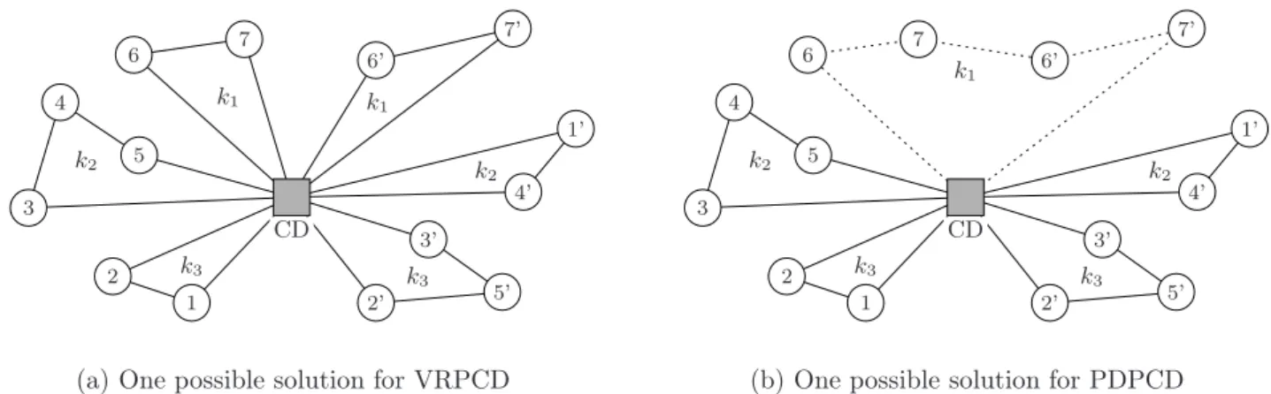
To further illustrate the differences between the two types of routes, in Figures
2.2a and 2.2b we depict two sets of 3 routes. In Figure 2.2a, only docking routes are used. In Figure 2.2b, routes of both types are considered. Note that, in Figure 2.2b, the route implemented by vehiclek1 visits customer 6′ right after collecting request p7
at supplier 7. Therefore, vehicle k1 delivers and collects the same set of products and
1 2 3
4 5
6 7 6’
7’ 2’ 3’ 5’ 1’ 4’ CD
k1 k1
k2 k
2
k3
k3
(a) One possible solution for VRPCD
1 2 3
4 5
6 7 6’
7’ 2’ 3’ 5’ 1’ 4’ CD k1
k2 k
2
k3
k3
(b) One possible solution for PDPCD
Figure 2.2: Differences between possible solutions for VRPCD and PDPCD, with K= 3, n= 7. In the figures, k1,k2 and k3 denote routes.
Depending on the geographical distribution of suppliers and customers and on how loading/unloading costs compare to arc costs, optimal solutions to PDPCD may involve both types of routes or not. If loading/unloading operations are too costly, optimal PDPCD solutions are likely to include more pickup and delivery routes. On the contrary, if load changing costs are zero, docking routes should be selected more frequently.
Compared to other routing models that integrate cross-docking with vehicle rout-ing in the literature, the introduction of pickup and delivery routes allowed substantial reductions in the transportation costs. In the worst case, solutions for the PDPCD have the same cost of those obtained for VRPCD (whether no pickup and delivery routes are used).
2.4
The Two-Echelon Capacitated Vehicle Routing
Problem
In turn, the design of integrated methods for the distribution of goods poses several new challenges, from an optimization perspective. For example, optimization models and algorithms have to explicitly take into account the possibility of consolida-tion of loads of several carriers in different warehouses and the coordinaconsolida-tion of shared freights in charge of deliverying goods to final customers.
One successful approach for the integrated transportation of goods in urban areas is the multi-echelon transportation system. It consists in using intermediate warehouses to consolidate the shipment of products from one or more depots or suppliers to final customers [Ricciardi et al., 2002; Topan et al., 2009]. In a multi-echelon system, the direct flow of goods from suppliers to the final destination is not allowed. Instead, factories, depots, warehouses and customers are organized in layers (or levels) and only the transportation of goods from/to entities in the same layer is allowed. One advantage of multi-echelon systems is that vehicles in each layer can be conveniently sized in order to satisfy regulations imposed on cargo transportation in specific urban areas.
Layers in multi-echelon systems are usually set according to the problem to be solved. The most common choice is the two-echelon system, where intermediate de-pots, named satellites, are placed between suppliers and final customers [Crainic et al.,
2010; Jung and Mathur, 2009]. In such a system, goods are shipped (usually in large quantities) from the central depot (supplier) to the satellites, where the consolidation of goods takes place. That means that products are moved to smaller trucks in order to be delivered to their final destinations. The consolidation of goods at the satellites is a quite effective tool for improving efficiency of transportation systems in urban areas. One the one hand, it allows goods supplied by different providers to be transported together, to destinations that are either the same or that lie close to each other. On the other, it allows goods to be placed in vehicles of size and weight suitable to the regions these goods are going to be delivered.
depends on the distance traveled by the vehicles) and the cost of consolidating goods at the satellites. In many cases, 2E-CVRP aims at finding a collection of routes with minimum total cost (traveling plus consolidation costs).
In what follows we formalize the 2E-CVRP. To that end, let G = (V, A) be digraph with set of vertices V := {{0}, S, C}, where 0 is a depot, S := {s1, . . . , sk}
and C := {c1, . . . , cn} denote respectively sets of satellites and customers. Assume
that, the arcs set A is partitioned into disjoint subsets A1 and A2, such that A :=
A1 ∪A2(A1 ∩A2 = ∅). On the one hand, level-1 arcs, which connect the satellites
and the depot, is given by set A1 := {(i, j) : i, j ∈ {0} ∪S}. On the other hand,
A2 :={(i, j) :i, j ∈C} ∪ {(i, j) :i∈S, j ∈C ori∈C, j ∈S} denotes the set of
level-2 arcs, which connect customers and satellites. A fleet K1 of K1 =|K1| homogeneous
vehicles with capacity q1 is in charge to implement level-1 routes, while level-2 routes
are implemented by a fleet K2 ofK2 =|K2|homogeneous vehicles with capacityQ2. To
each customeri∈C, an amount di >0of the same good must be delivered. Whenever
an arc (i, j)∈ A is traversed by a vehicle, a cost cij is incurred. In addition, for each
unit of good which passes on satellite s a cost Ls is going to be paid. The goal in
2E-CVRP is to assign up to K1 level-1 routes and up toK2 level-2 routes to ship goods
from the depot the their respective customers. On the level-2 a given customer must be visited exactly once, while on the level-1 a given satellite may be visited n times (n ≥0).
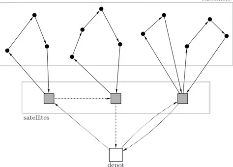
In Figure 2.3, we depict routes involved in a 2E-CVRP solution. In the figure, coloured circles represent elements of C, while colored squares denote elements of S. The picture indicates a collection of routes spanning 3 satellites, 12 customers and a single depot. Note that, there is no direct connection between the depot and customers. The transportation of goods follows the arcs in the digraph and only takes place between the depot and satellites and from there to the customers. Goods shipped from the depot must stop at satellites, where loads are consolidated into smaller vehicles. Accordingly, two types of routes are indicated. Those in the lower part of the picture, named level-1 routes, connect the depot to the satellites. The others, on the upper part, are named level-2 routes. They connect one single satellite to one or more customers.
As VRPs, various types of constraints associated with the routing and the con-solidation of loads define some 2E-CVRP variants. In the literature, some authors interchangeably use the terms 2E-CVRP and 2E-VRP to refer to the basic version of problem, where only capacity constraints are considered. According to Perboli et al.
depar-depot
customers
satellites
Figure 2.3: Example of solution for the 2E-VRP
ture of vehicles at the satellites are considered. In both problems, the 2E-VRP-TW and the 2E-VRP-SS, time windows constraints may be hard or soft. There are also the multi-depot 2E-VRP where loads can departure from more than one depot to satisfy customers demand. Finally, the 2E-VRP with Taxi Services (2E-VRP-TS) allows some loads to be shipped directly from the depot to customers, bypassing satellites.
From a computational point of view, solving 2E-CVRP is not a trivial task. That applies since the Capacitated Vehicle Routing Problem (CVRP), a widely known NP-hard optimization problem, can be seen as a 2E-CVRP special case, with only one depot and satellite. The first exact solution approach for the 2E-CVRP was introduced by Perboli et al. [2008b, 2011]. The authors proposed an Integer Programming (IP) formulation based on network flows. Such a formulation consists of defining flows from the depot to satellites and from there to customers. Variables f1
ij and fij2s define the
flow on the level-1 and level-2, respectively. Similarly, arc variables x1
ij represent the
number of level-1 vehicles using arc (i, j) ∈ A1 and binary variables x2ijs represent
whether an arc is used or not for routing on level-2. Finally, variables zsi assume value
1 if and only if the demand of a given customer i∈ C pass through a satellite s ∈ S