13
Logistics: The Vehicle Routing Problem
Competition is the keen cutting edge of business, always shaving away at costs.
Henry Ford (1863 - 1947) – Businessman
Transportation plays an important role in logistic tasks of many companies since it usually accounts for a high percentage of the cost added to goods. Therefore, the use of computerized methods in transportation often results in significant savings of up to 20% of the total costs (see Chap. 1 in [248]).
A distinguished problem in the field of transportation consists in finding the optimal routes for a fleet of vehicles which serve a set of clients. In this problem, an arbitrary set of clients must receive goods from a central depot. This general scenario presents many chances for defining (related) problem scenarios, for example: determining the optimal number of vehicles, finding the shortest routes, and so on, being all of them subject to many restrictions such as vehicle capacity, time windows for deliveries, etc. This variety of scenarios leads to a plethora of problem variants in practice. Some reference case studies where the application of vehicle routing algorithms has led to substantial cost savings can be found in Chaps. 10 and 14 in [248].
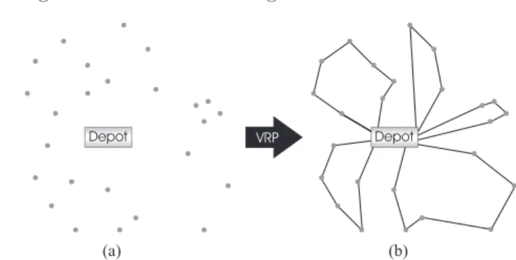
As stated before, the vehicle routing problem (VRP) [56] consists of deliv-ering goods to a set of customers with known demands through minimum-cost vehicle routes. These routes must start and finish at the depot, as can be seen in Figs. 13.1a and 13.1b (a detailed description of the problem is available in Sect. 13.1).
The VRP is a very important source for problems, since solving it is equiv-alent to solving multiple TSP problems at once [96]. Due to the difficulty of this problem (NP-hard) and because of its many industrial applications, it has been largely studied both theoretically and in practice [47]. There is a large number of extensions to the canonical VRP. One basic extension is known as the capacitated VRP –CVRP–, in which vehicles have fixed capacities of a single commodity. Many different variants can be constructed from CVRP; some of the most important ones [248] are those including time windows re-strictions –VRPTW– (customers must be supplied following a certain time schedule), pickups and deliveries –VRPPD– (customers will require goods to be either delivered or picked up), and backhauls –VRPB– (like VRPPD, but deliveries must be completed before any pickups are made).
E. Alba, B. Dorronsoro,Cellular Genetic Algorithms,
Depot VRP Depot
(a) (b)
Fig. 13.1.The vehicle routing problem consists in serving a set of geographically distributed customers (points) from a depot (a) using the minimum cost routes (b)
In fact, there are many more extensions for this problem, like the use of multiple depots (MDVRP), split deliveries (SDVRP), stochastic variables (SVRP), or periodic scheduling (PVRP). The reader can find a public web site with all of them, the latest best-known solutions, papers and related stuff in our web site [71].
We consider in this chapter the capacitated vehicle routing problem (CVRP), in which a fixed fleet of delivery vehicles of the same capacity must service known customer demands for a single commodity from a common de-pot at minimum transit costs. The CVRP has been studied in a large number of separate works in the literature, but (to our knowledge) no work addresses all the available benchmarks together, since it means solving 160 different instances. We use such a large set of instances to test the behavior of our algorithm in many different scenarios in order to give a deep analysis of it and a general view of this problem not biased by any ad hoc selection of indi-vidual instances. The included instances are characterized by many different features: instances from real world, theoretically motivated ones, clustered, non-clustered, with homogeneous or heterogeneous demands on customers, with the existence of drop times or not, etc.
13.1 The Vehicle Routing Problem 177
The contribution of this work is then to define a powerful yet simple cMA capable of competing with the best known approaches for solving CVRP in terms of accuracy (final cost) and computational effort (the number of evalua-tions made). For that purpose, we test our algorithm over the mentioned large selection of instances (160), which will allow us to guarantee deep and mean-ingful conclusions. Besides, we compare our results against the best existing ones in the literature, some of which we even improve. In [11] the reader can find a seminal work with a comparison between our algorithm and some other known heuristics for a reduced set of 8 instances. In that work, we showed the advantages of embedding local search techniques into a cGA for solving CVRP, since our hybrid cGA was the best algorithm out of all those compared in terms of accuracy and time. Cellular GAs represent a paradigm much simpler to comprehend and customize than others such as tabu search (TS) [97, 249] and similar (very specialized or very abstract) algorithms [37, 207]. This is an important point too, since the greatest emphasis on simplicity and flexibility is nowadays a must in research to achieve widely useful contributions [52].
The chapter is organized in the following manner. In Sect. 13.1 we define CVRP. The proposed cMA is thoroughly described in Sect. 13.2. Section 13.3 presents the results of our tests, comparing them with the best-known values in the literature. After that, we present the new best-known solutions found in our studies for CVRP in Sect. 13.4. Finally, our conclusions and future lines of research are discussed in Sect. 13.5.
13.1 The Vehicle Routing Problem
The VRP can be defined as an integer programming problem which falls into the category of NP-hard problems [161]. Among the different variants of VRP we work here with the Capacitated VRP (CVRP), in which every vehicle has a uniform capacity of a single commodity. The CVRP is defined on an undirected graphG= (V,E) whereV={v0, v1, . . . , vn} is a vertex set and
E={(vi, vj)/vi, vj∈V, i < j} is an edge set.
Vertexv0 stands for thedepot, and it is from where m identical vehicles of capacityQ must serve all thecities or customers, represented by the set of n vertices {v1, . . . , vn}. We define on E a non-negative cost, distance or
travel time matrixC = (cij) between customersvi andvj. Each customervi has non-negative demand of goodsqiand drop timeδi(time needed to unload all goods). LetV1, . . . ,Vm be a partition ofV, a routeRiis a permutation
of the customers in Vi specifying the order of visiting them, starting and
finishing at the depotv0. The cost of a given route Ri={vi0, vi1, . . . , vik+1},
wherevij ∈Vandvi0=vik+1 = 0 (0 denotes the depot), is given by:
Cost(Ri) =
k X
j=0
cj,j+1+ k X
j=0
δj, (13.1)
FCVRP(S) = m X
i=1
Cost(Ri). (13.2)
CVRP consists in determining a set ofmroutes (i) of minimum total cost –as it is specified in Eq. 13.2–; (ii) starting and ending at the depotv0; and such that (iii) each customer is visited exactly once by exactly one vehicle; subject to the restrictions that (iv) the total demand of any route does not exceed Q (P
vj∈Riqj ≤ Q); and (v) the total duration of any route is not
larger than a preset boundD (Cost(Ri) ≤ D). All vehicles have the same
capacity and carry a single kind of commodity. The number of vehicles is either an input value or a decision variable. In this study, the length of routes is minimized independently of the number of vehicles used.
It is clear from our description that the VRP is closely related to two difficult combinatorial problems. On the one hand, we can get an instance of
theMultiple Travelling Salesman Problem(MTSP) just by settingQ=∞. An
MTSP instance can be transformed into a TSP instance by adjoining to the graphk−1 additional copies of node 0 (depot) and its incident edges (there are no edges among the kdepot nodes). On the other hand, the question of whether there exists a feasible solution for a given instance of the VRP is an instance of theBin Packing Problem (BPP). So the VRP is extremely difficult to solve in practice because of the interplay of these two underlying difficult models (TSP and BPP). In fact, the largest solvable instances of the VRP are two orders of magnitude smaller than those of the TSP [208].
13.2 Proposed Algorithms
In this section we present a detailed description of the operators we imple-mented in our algorithm (for a complete description of the algorithm itself the reader should refer to Chap. 1). In Alg. 13.1 the pseudo-code of JCell2o1i, the cMA we propose in this study, is given. Basically, we use a simple cGA highly hybridized with specific recombination and mutation operators, and also with an added local post-optimization step (line 12). This local search method lies in applying1-Interchange, and then improving the best obtained solution using 2-Opt. These two methods are well-known local search optimization algorithms in the literature (they are described in detail in Sect. 13.2.4).
The fitness value assigned to individuals is computed as follows [11, 97]:
f(S) =FCVRP(S) +λ·overcap(S) +µ·overtm(S), (13.3)
13.2 Proposed Algorithms 179
Algorithm 13.1Pseudo-code of JCell2o1i
1. procEvolve(cma) //Algorithm parameters in ‘cma’ 2. GenerateInitialPopulation(cma.pop);
3. Evaluation(cma.pop); 4. while!StopCondition()do
5. forindividual ← 1tocma.popSizedo
6. neighbors ←GetNeighbors(cma,position(individual)); 7. parents←Select(neighbors);
8. offspring←Recombination(cma.Pc,parents); 9. offspring←Mutation(cma.Pm,offspring); 10. offspring←LocalSearch(cma.Pl,offspring); 11. Evaluation(offspring);
12. InsertIfNotWorse(position(x,y),offspring,cma,aux pop); 13. end for
14. cma.pop←aux pop; 15. UpdateStatistics(cma); 16. end while
17. end procEvolve;
The objective of our algorithm is to maximizefeval(S) (Eq. 13.4) by min-imizingf(S) (Eq. 13.3). The valuefmax must be larger or equal with respect to that of the worst feasible solution for the problem. Functionf(S) is com-puted by adding the total costs of all the routes (FCVRP(S) –see Eq. 13.2–), and penalizes the fitness value only in the case that the capacity of any ve-hicle and/or the time of any route are exceeded. Functions ‘overcap(S)’ and ‘overtm(S)’ return the excess in capacity and time of the solution (respec-tively) with respect to the maximum allowed value for each route. The values returned by ‘overcap(S)’ and ‘overtm(S)’ are weighted by factors λ and µ, respectively. In this work we have usedλ=µ= 1000 [78].
In Sects. 13.2.1 to 13.2.4 we proceed to explain in detail the main features that characterize our algorithm (JCell2o1i). The algorithm itself can be ap-plied with all the mentioned operations and also with only some of them to analyze their separate contribution to the performance of the search, as it was previously done for this algorithm in [14].
13.2.1 Problem Representation
4 - 5 - 2 - 10 - 0 - 3 - 1 - 12 - 7 - 8 - 9 - 11 - 6
{
{
{
{
Route 1 Route 2 Route 3 Route 4
Route Splitters
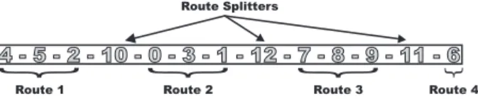
Fig. 13.2.Individual representing a solution for 10 customers and 4 vehicles
are represented with numbers [0. . . c−1], while route splitters belong to the range [c . . . n−1]. Note that due to the nature of the chromosome (permuta-tion of integer numbers) route splitters must be different numbers, although it should be possible to use the same number for designating route splitters when using other possible chromosome configuration.
Each route is composed of the customers between two route splitters in the individual. For example, in Fig. 13.2 we plot an individual representing a possible solution for a hypothetical CVRP instance with 10 customers using at most 4 vehicles. Values [0, . . . ,9] represent the customers while [10, . . . ,12] are the route splitters.Route 1 begins at the depot, visits customers 4–5–2 (in that order), and returns to the depot.Route 2 goes from the depot to customers 0–3–1 and returns. The vehicle ofRoute 3starts at the depot and visits customers 7–8–9. Finally, inRoute 4, only customer 6 is visited from the depot. Empty routes are allowed in this representation simply by placing two route splitters contiguously without any client between them.
13.2.2 Recombination
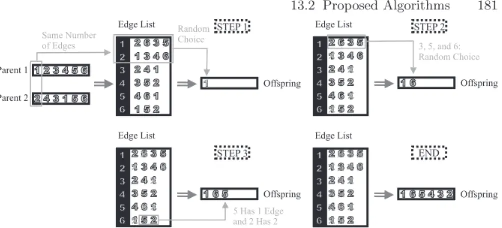
Recombination is used in GAs as an operator for combining parts in two (or more) patterns in order to transmit (hopefully) good building blocks in them to their offspring. The recombination operator we use is the edge recombi-nation operator (ERX) [262], since it has been largely reported as the most appropriate for permutations compared to other general operators like order crossover (OX) or partially matched crossover (PMX). ERX builds an off-spring by preserving edges from its two parents. For that, anedge list is used. This list contains, for each city, the edges of the parents that start or finish in it (see Fig. 13.3).
13.2 Proposed Algorithms 181
2 6 3 5
1 3 4 6
2 4 1
3 5 2
4 6 1
1 5 2 Edge List
1 6 5 Offspring 1 2 3 4 5 6
5 Has 1 Edge and 2 Has 2 2 6 3 5
1 3 4 6
2 4 1
3 5 2
4 6 1
1 5 2 Edge List
1 2 3 4 5 6 Parent 1 Parent 2 1 Offspring 1 2 3 4 5 6 2 4 3 1 5 6
Same Number of Edges
Random Choice
STEP 1
2 6 3 5
1 3 4 6
2 4 1
3 5 2
4 6 1
1 5 2 Edge List
1 6 Offspring 1 2 3 4 5 6
3, 5, and 6: Random Choice
STEP 2
STEP 3 2 6 3 5 1 3 4 6
2 4 1
3 5 2
4 6 1
1 5 2 Edge List
1 6 5 4 3 2 Offspring 1 2 3 4 5 6 END
Fig. 13.3.Edge recombination operator (ERX)
13.2.3 Mutation
The mutation operator we use in our algorithm will play an important role during the evolution since it is in charge of introducing a considerable degree of diversity in each generation, counteracting in this way the strong selective pressure which is a result of the local search method we plan to use. The mutation consists of applyingInsertion,SwaporInversion operations to each gene with equal probability (see Alg. 13.2).
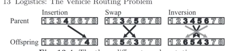
These three mutation operators (see Fig. 13.4) are well-known methods found in the literature, and typically applied sooner than later in rout-ing problems. Our idea here is to merge they three in a new combined
operator. The Insertion operator [89] selects a gene (either customer or route splitter) and inserts it in another randomly selected place of the same individual. Swap [36] lies in randomly selecting two genes in a so-lution and exchanging them. Finally, Inversion [134] reverses the visiting order of the genes between two randomly selected points of the
permuta-Algorithm 13.2The mutation algorithm
1. procMutation(pm, ind)
// ‘pm’ is the mutation probability, and ‘ind’ is the individual to mutate 2. fori←1toind.length()do
3. if rand0to1()<pmthen
4. r =rand0to1(); 5. if r<0.33then
6. ind.Inversion(i,randomInt(ind.length())); 7. else if r>0.66then
8. ind.Insertion(i,randomInt(ind.length()));
9. else
10. ind.Swap(i,randomInt(ind.length())); 11. end if
12. end if
13. end for
1 2 345 6 7 8 1 2 3 5 6 748
1 23456 7 8 1 25436 7 8
1 23 4 5 67 8
1 26 5 4 37 8
Inversion Swap
Insertion Parent
Offspring
Fig. 13.4.The three different used mutations
tion. Note that the induced changes might occur in an intra or inter-route way in all the three operators. Formally stated, given a potential solution
S={s1, . . . , sp−1, sp, sp+1, . . . , sq−1, sq, sq+1, . . . , sn}, wherepand qare ran-domly selected indexes, andnis the sum of the number of customers plus the number of route splitters (n=c+k), then the new solutionS′
obtained after applying each of the different proposed mechanisms is shown below:
Insertion : S′={s
1, . . . , sp−1, sp+1, . . . , sq−1, sq, sp, sq+1, . . . , sn}, (13.5)
Swap : S′={s
1, . . . , sp−1, sq, sp+1, . . . , sq−1, sp, sq+1, . . . , sn}, (13.6)
Inversion : S′={s
1, . . . , sp−1, sq, sq−1, . . . , sp+1, sp, sq+1, . . . , sn}. (13.7)
13.2.4 Local Search
It is very clear after all the existing literature on VRP that the utilization of a local search method is almost mandatory to achieve results of high quality [11, 37, 217]. This is why we envision from the beginning the application of two of the most successful techniques in recent years. In effect, we will add a local refining step to some of our algorithms consisting in applying 2-Opt [55] and 1-Interchange [200] local optimization to every individual.
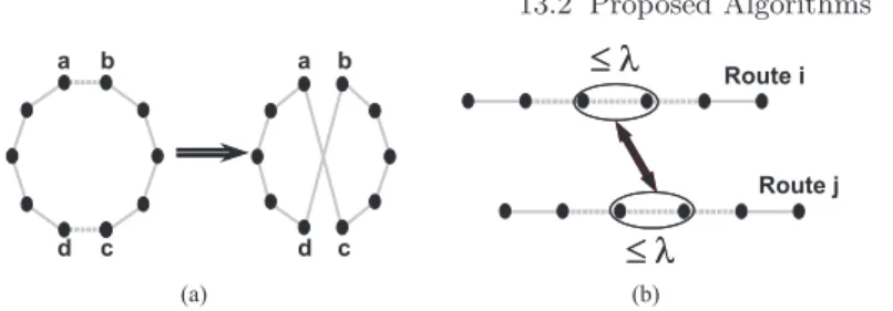
On the one hand, the 2-Opt simple local search method works inside each route. It randomly selects two non-adjacent edges (i.e., (a, b) and (c, d)) of a single route, deletes them, thus breaking the tour into two parts, and then reconnects those parts in the other possible way: (a, c) and (b, d) (Fig. 13.5a). Hence, given a routeR={r1, . . . , ra, rb, . . . , rc, rd, . . . , rn}, being (ra, rb) and (rc, rd) two randomly selected non-adjacent edges, the new routeR′obtained after applying the 2-Opt method to the two considered edges will be R′
= {r1, . . . , ra, rc, . . . , rb, rd, . . . , rn}. 2-Opt is similar to the inversion mutation operator with the exception that 2-Opt is applied into routes, whileinversion
can affect one or more routes.
On the other hand, theλ-Interchange local optimization method that we use is based on the analysis of all the possible combinations for up to λ
customers between sets of routes (Fig. 13.5b). Hence, this method results in customers either being shifted from one route to another, or being exchanged between routes. The mechanism can be described as follows. A solution to the problem is represented by a set of routesS ={R1, . . . , Rp, . . . , Rq, . . . , Rk}, whereRiis the set of customers serviced in routei. New neighboring solutions can be obtained after applyingλ-Interchange between a pair of routesRp and
Rq; to do so we replace each subset of customers S1 ⊆Rp of size|S1| ≤ λ with any other oneS2 ⊆ Rq of size |S2| ≤ λ. This way, we obtain two new routesR′
p = (Rp−S1) S
S2 and R′q = (Rq−S2) S
S1, which are part of the new solutionS′
={R1. . . R′p. . . R
′
13.2 Proposed Algorithms 183
Fig. 13.5.2-Opt works into a route (a), whileλ-Interchange affects two routes (b)
Therefore, 2-Opt searches for better solutions by modifying the order of visiting customers inside a route, while theλ-Interchange method results in customers either being shifted from one route to another, or customers being exchanged between routes. This local search step is applied to an individual after the recombination and mutation operators, and returns the best solution between the best ones found by 2-Opt and 1-Interchange, or the current one if it is better (see a pseudo-code in Alg. 13.3). In the local search step, the algorithm applies 2-Opt to all the pairs of non-adjacent edges in every route and 1-Interchange to all the subsets of up to 1 customer between every pair of routes.
Algorithm 13.3The local search step
1. procLocal Search(ind) // ‘ind’ is the individual to improve 2. fors← 0toMAX STEPS do
3. //First: 2 Opt.K is the number of routes.MAX STEPS = 20 4. best2 Opt = ind;
5. forr ← 0toKdo
6. sol =2 Opt(ind,r);
7. if Best(sol,best2 Opt)then
8. best2 Opt = sol;
9. end if
10. end for
11. end for
12. //Second: 1 Interchange. 13. best1 Interchange = ind; 14. fors← 0toMAX STEPS do
15. fori← 0toLength(ind)do
16. forj← i+1toLength(ind)do
17. sol =1 Interchange(i,j);
18. if Best(sol,best1 Interchange)then
19. best1 Interchange = sol;
20. end if
21. end for
22. end for
23. end for
In summary, the functioning of JCell is quite simple: in each generation, an offspring is obtained for every individual after applying the recombination operator (ERX) to its two parents (selected from its neighborhood). The off-springs are mutated with a special combined mutation, and later a local post-optimization step is applied to the mutated individuals. This local search algorithm consists in applying to the individual two different local search methods (2-Opt and 1-Interchange), and returns the best individual among the input individual and the output of 2-Opt and 1-Interchange. The popula-tion of the next generapopula-tion will be composed of the current one after replacing its individuals with their offsprings in the cases where they are better.
13.3 Solving CVRP with JCell2o1i
In this section we describe the results of the experiments we have made for testing our algorithm on CVRP. JCell2o1i has been implemented in Java and tested on a Pentium IV 2.8 GHz PC with Linux on a very large test suite, com-posed of an extensive set of benchmarks drawn from the literature: (i) Augerat
et al. (sets A, B and P) [29], (ii) Van Breedam [252], (iii) Christofides and
Eilon [46], (iv) Christofides, Mingozzi and Toth (CMT) [47], (v) Fisher [87], (vi) Goldenet al.[109], (vii) Taillard [240], and (viii) a benchmark generated from TSP instances [212]. All these benchmarks, as well as the best-known solution for their instances, are publicly available at [71].
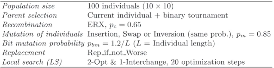
Due to the heterogeneity of this huge test suite, we will find many different features in the studied instances, which will represent a hard test to JCell2o1i for this problem, usually much larger than usual studies in the VRP literature. The parameterization used in this study for JCell2o1i (listed in Table 13.1) is the same for the 160 instances of our benchmark with the only exception of the maximum allowed number of evaluations of the termination condition. This value was fixed in terms of the length and difficulty of the instances. All the numerical results of the algorithm (optimal routes, costs, etc.) for every problem are available in [14]. These results were obtained after making 100 independent runs (in order to obtain statistical confidence), except for the case of the benchmark by Golden et al., for which 30 runs were made due to the high computational requirements of these problems.
Table 13.1. Parameterization used in JCell2o1i
Population size 100 individuals (10×10)
Parent selection Current individual + binary tournament
Recombination ERX,pc= 0.65
Mutation of individuals Insertion, Swap or Inversion (same prob.),pm= 0.85 Bit mutation probabilitypbm= 1.2/L (L= Individual length)
Replacement Rep if not Worse
13.4 New Solutions to CVRP 185
Table 13.2.Average deviation between our best solution found and the best known one for all the instances of every studied benchmark
Benchmark Avg.∆ Augerat et al. Set A 0.00 Augerat et al. Set B 3.48e−03
Augerat et al. Set P 0.00
Van Breedam 2.45
Christofides & Eilon 0.00
CMT 0.29
Fisher 0.00
Golden at al. 1.44
Taillard 0.56
Extended from TSP 0.00
We show in Table 13.2 the average deviations obtained between our best obtained solution (sol) and the best known one (best) for all the instances of every benchmark. This deviation (∆) is computed as shown in Eq. 13.8.
∆(sol) =
best−sol best
·100 . (13.8)
Following the TSPLIB convention [212], distances between customers have been rounded to the closest integer value in instances belonging to the bench-marks of Augerat et al., Van Breedam, Christofides and Eilon, Fisher, and the set of translated instances from TSP.
As it can be seen in Table 13.2, the average errors obtained by JCell2o1i for every benchmark are very low, with values always under 1.5%. Note that the
boldedresult for Van Breedam’s benchmark corresponds to an improvement of our results with respect to the previously existing ones. Thus, JCell2o1i has demonstrated to be a robust algorithm highly suitable for VRP on a large testbed.
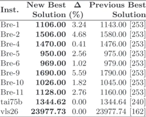
13.4 New Solutions to CVRP
Table 13.3.New best solutions found
Inst. New Best ∆ Previous Best Solution (%) Solution
Bre-1 1106.00 3.24 1143.00 [253] Bre-2 1506.00 4.68 1580.00 [253] Bre-4 1470.00 0.41 1476.00 [253] Bre-5 950.00 2.56 975.00 [253] Bre-6 969.00 1.02 979.00 [253] Bre-9 1690.00 5.59 1790.00 [253] Bre-10 1026.00 1.82 1045.00 [253] Bre-11 1128.00 2.76 1160.00 [253] tai75b 1344.62 0.00 1344.64 [240] vls26 23977.73 0.00 23977.74 [162]
13.5 Conclusions
In this chapter we have developed a single algorithm which is able to compete with the many different best known optimization techniques for solving the CVRP. Our algorithm has been tested in a very large set of 160 instances with different features, e.g., uniformly and not uniformly dispersed customers, clus-tered and not clusclus-tered, with a cenclus-tered or not cenclus-tered depot, having maximal route distances or not, considering drop times or not, with homogeneous or heterogeneous demands, etc.
We consider that the behavior of our cellular algorithm with merged mu-tation plus local search is very satisfactory since it obtains the best-known solution in most cases, or values very close to it, for all of the test suite. Moreover, it has been able to improve the known best solution so far for nine of the tested instances, which represents an important record in present re-search. Hence, we can say that the performance of JCell2o1i is similar or even better to that of the best algorithm for each instance. Besides, our algorithm is quite simple since we have designed a canonical cGA with three widely used mutations in the literature for this problem, plus two well-known local search methods.