Burrows-Wheeler Transform in Secondary Memory

(1)

Universidade Nova de Lisboa

Faculdade de Ciências e Tecnologia

Departamento de Informática

Master’s Thesis in Computer Engineering 2nd Semester, 2009/2010

Burrows-Wheeler Transform in Secondary Memory

28038 Sérgio Miguel Cachucho Pereira

Advisor

Professor Luís Manuel Silveira Russo

(2)

(3)

Student Number: 28038

Name: Sérgio Miguel Cachucho Pereira

Dissertation Title:

Burrows-Wheeler Transform in Secondary Memory

Keywords:

 Suffix arrays  External sorting  Heap

 Pattern matching  Indexes

Palavras-Chave:

 Arrays de sufixos

 Ordenação em memória secundária  Heap

(4)

(5)

Abstract

(6)

(7)

Resumo

(8)

(9)

Table of Figures

Figure 1. Example of how to obtain the suffix array of a given text. ... 5

Figure 2. Example of the Burrow-Wheeler Transform. ... 6

Figure 3. Example of the isomorphism between Quicksort and binary search trees. ... 8

Figure 4. The ternary search tree of the example of Figure 3. ... 9

Figure 5. Example of the Quickheap. ... 13

Figure 6. Example of inserting a new element in a Quickheap. ... 16

Figure 7. Definition of three different terms related to the LCP. ... 17

Figure 8. The Doubling Algorithm and its pipeline representation. ... 19

Figure 9. The DC3-algorithm. ... 21

Figure 10. The data-flow graph for the DC3-algorithm. ... 22

Figure 11. Illustration of the splitting part of our algorithm. ... 25

Figure 12. Illustration of the merging part of our algorithm. ... 27

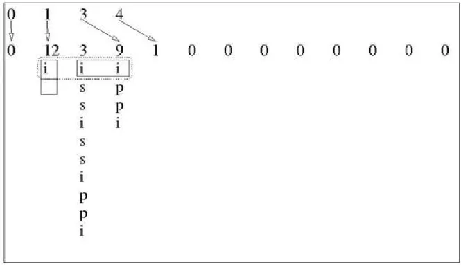
Figure 13. Suffixes and the respective indexes for the text “mississippi”. ... 44

Figure 14. Representation of the heap data structures after inserting the first three suffixes. ... 46

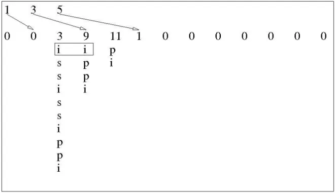
Figure 15. Representation of the heap data structures before extracting the first suffix (12). ... 47

Figure 16. Representation of the heap data structures after inserting a new suffix (11). ... 48

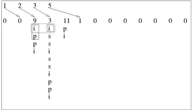
Figure 17. Representation of the heap data structures before extracting a suffix (9). ... 49

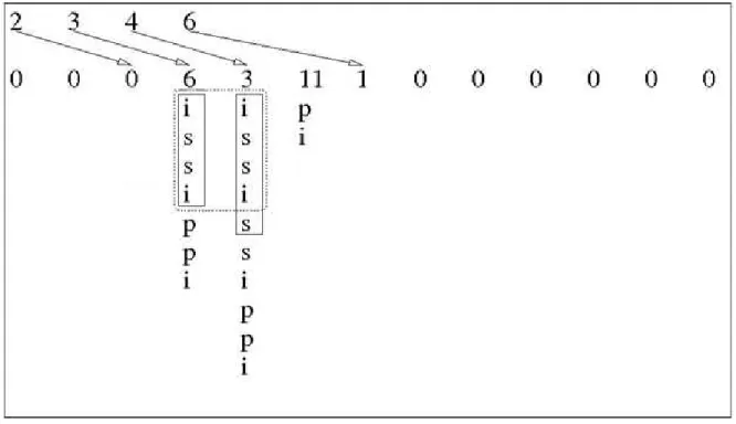
Figure 18. Representation of the heap data structures before inserting a new suffix (6). ... 49

Figure 19. Representation of the heap data structures before extraction of a suffix (6). ... 50

Figure 22. Representation of the heap after all extractions.... 52

Figure 23. Table with the experimental results for different values of partial suffix arrays. ... 54

Figure 24. Chart illustrating the data from Figure 23 that refers to memory usage. ... 54

Figure 25. Chart illustrating the data from Figure 23 that refers to running time. ... 55

(12)

Figure 27. Chart showing the data from Figure 26 that refers to memory usage. ... 57

Figure 28. Table with the experimental results for different numbers of suffixes in the heap. ... 58

Figure 29. Chart with the data from Figure 28 that refers to memory usage. ... 59

Figure 30. Chart with the data from Figure 28 that refers to running time. ... 59

Figure 31. Table with the experimental results for different LCP values. ... 61

Figure 32. Chart showing the data from Figure 31 that refers to the memory usage. ... 61

Figure 33. Chart showing the data from Figure 31 that refers to the running time. ... 62

Figure 34. Table with the experimental results for the three algorithms with the file dblp.xml.100MB. ... 64

Figure 35. Chart showing the data from Figure 34 that refers to the heap without blocks. ... 65

Figure 36. Chart showing the data from Figure 34 that refers to the heap with blocks.... 65

Figure 37. Chart showing the data from Figure 34, comparing the running times of the three algorithms, and the merging part of both versions of our algorithm. ... 66

Figure 38. Table with the experimental results for the three algorithms with the file dna.100MB. ... 67

Figure 42. Table with the experimental results for the three algorithms with the file proteins.100MB. ... 70

(13)

(14)

(15)

1. Introduction

1.1Motivation

Nowadays text processing is a significant and fast expanding area within computer science. There are several applications, studies and research areas that depend on the existence of fast text processing algorithms. One such area is biology. Having machines that automatically search a DNA sequence and look for patterns in a short amount of time is essential for researchers, and has greatly contributed to important discoveries that would otherwise be impossible. These machines use sophisticated text processing algorithms, capable of handling long DNA sequences in a very short time. Another research area that requires algorithms is automated text translation. Like in the previous example, it also needs to process text in very limited amounts of time, as well as to look for patterns at the same time.

These algorithms are most of the times built on top of some state-of-the-art string processing data structures. One such structure is the suffix array, which is an array containing all the suffixes of a given text, in lexicographical order. This makes the process of looking for a pattern much more efficient, since the suffixes related to the query are stored in consecutive positions in the array. Furthermore being sorted makes it possible to use an O( logn ) algorithm to look for a

(16)

The main setback of suffix arrays is that most of the existing algorithms that use secondary memory are only appropriate for quite small input texts, which in many cases makes them less suitable to solve certain problems. This happens mainly because those algorithms need to store all the suffixes in main memory, alongside with the text, which obviously restricts them to be used only with texts that are much smaller than the memory of the computer where it will be processed. As mentioned before, the use of suffix arrays makes certain operations much faster, which is especially significant with problems that require handling large texts, such as processing a DNA sequence or a book. Although, most of the current implementations of algorithms to build suffix arrays using secondary memory can’t themselves handle large input texts, reason why the use of suffix arrays are yet to reach its full potential.

This work aims to improve this situation. We will propose an algorithm that builds the suffix array for a given text, but that doesn’t need all the suffixes to be stored in main memory at the same time, instead just a small part of them will, all others will remain in secondary memory. Achieving this goal will make the use of suffix arrays wider, especially for those problems that require handling large amounts of data.

1.2Problem Description

Since suffix arrays are very useful indexes to solve problems that require handling text and looking for patterns in it, the motivation for building suffix arrays is clearly established, and this is the main focus of this work. A very important side effect that can be obtained from our approach is the computation of the Burrows-Wheeler transform of the text, which is a crucial piece for more sophisticated compressed indexes.

(17)

There are two issues to be taken into account when building suffix arrays: to be space-conscious and streaming. We define a space-conscious solution as one that doesn’t need to store the whole working data in main memory, using for that purpose the secondary memory. In the context of the suffix arrays, a solution that stores in main memory both the text and the suffix array is not an example of a space-conscious solution. Otherwise, a solution, like ours, that stores in main memory only the text and a small part of the suffixes, keeping the rest of the suffixes in secondary memory is a space-conscious solution.

A streaming solution is one that runs from the beginning of its execution up to the end without blocking. The use of secondary memory raises the issue of blocking I/Os, because the disk access is dominant over main memory access in the complexity of these algorithms, thus at some point in the execution it has to block waiting for new data from the disk. However we want our algorithm to reduce this problem by defining an efficient I/O policy to prevent as much as possible our algorithm from blocking due to disk accesses.

(18)

2. Related Work

2.1Terminology

This work is about text and operations on it, hence strings are mentioned very often. In this context, a string and a text are the same thing, both mean a sequence of characters. When talking about strings, it is common to mention some related concepts. The size of a string is the number of characters it contains. The alphabet is the set containing all characters used in a text. Sorting, or ordering, is the process of arranging items in some ordered sequence. In this work will be used lexicographical order to sort the strings (suffixes) contained in a given array.

2.1.1 Suffix Arrays

One important focus of this work is to obtain the suffix array of a given text. A suffix of a text is a substring containing all the text characters from a given position up to the last one, in the exact same order as found in the given text. Moreover, a suffix array is a lexicographically sorted array, containing all the suffixes of a given text, thus a suffix array of a text with n characters is

an array containing its n suffixes sorted. The suffix array of a text is an array

containing a permutation of the interval , such that for all , where “ ” between strings is the lexicographical order [1].

(19)

Figure 1 contains an example of how to obtain the suffix array from a given text, in this case mississippi$. The illustration shows the original order of the suffixes of the text (on the left), and the resulting suffix array (on the right).

Text = mississippi$ Index Suffix

0 mississippi$ 1 ississippi$ 2 ssissippi$ 3 sissippi$ 4 issippi$ 5 ssippi$ 6 sippi$ 7 ippi$ 8 ppi$ 9 pi$ 10 i$ 11 $

Suffix Array = {11, 10, 7, 4, 1, 0, 9, 8, 6, 3, 5, 2}

Figure 1. Example of how to obtain the suffix array of a given text.

Puglisi et al. [6] made an extended researched about suffix arrays, from the origins until nowadays. Suffix arrays were introduced in 1990 by Manber & Myers, along with algorithms for their construction and use. From then to now suffix arrays have become the data structure of choice for solving many text processing problems. The designers of algorithms to build suffix arrays want them to have minimal asymptotic complexity, to be fast “in practice”, even with large real-world data inputs, and to be lightweight, which means use a small amount of working storage beyond the space used by the text. Until the date of this paper there are no algorithms that achieve all the three goals proposed.

Index Suffix 11 $ 10 i$

7 ippi$ 4 issippi$ 1 ississippi$ 0 mississippi$ 9 pi$

(20)

2.1.2 The Burrows-Wheeler Transform

The Burrows-Wheeler Transform (BWT) is a transformation from strings to strings that can be reversed. This operation makes the transformed text easier to compress, by local optimization methods, due to the much more frequent occurrence of repeated characters in the BWT than in the original text. The most usual way of getting the BWT of a text is by constructing its suffix array.

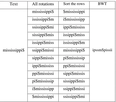
Figure 2. Example of the Burrow-Wheeler Transform. The BWT of the text “mississippi$” is “ipssm$pissii”.

As Figure 2 shows, obtaining the Burrows-Wheeler Transform of a given text is a simple process. The algorithm creates an array with size equal to the length of the text given. In the first position of that array is placed the original text and in the remaining positions are placed all the rotations possibly obtained from that text. By rotation I mean each character T[i] of the text go to

the position T[i-1], except the character T[0], which goes to the position T[n-1], where n is the

Text All rotations Sort the rows BWT mississippi$ $mississippi

ississippi$m i$mississipp ssissippi$mi ippi$mississ sissippi$mis issippi$miss issippi$miss ississippi$m

mississippi$ ssippi$missi mississippi$ ipssm$pissii sippi$missis pi$mississip

(21)

the possible rotations are obtained, except the original text, which is already in the first position of the array and would be obtained again in the n-th rotation. The second step of the algorithm is

to sort the rows that resulted from the rotations, i.e. sorting the resulting array by lexicographical order, which means that it is similar to a suffix array. The Burrows-Wheeler Transform of the text given is a string containing the last characters of each of the rotations, in the sorted order obtained in the second step. The string obtained in the end of the algorithm has the same size and contains the same characters as the original text, but in the BWT they are in a different order, according to the steps described.

If one compares Figure 2 with Figure 1, illustrating the BWT and the suffix array of a text, respectively, there are obvious similarities. In the first step, the rotations part, the BWT algorithm is equal to the suffix array construction, except that in the case of suffixes the first character of the text is dropped instead of moved to the end of the text. Yet the structure is exactly the same. The second step, the sorting part, is common to both the BWT and the suffix array construction. The last part, extracting the last characters to make the resulting string is exclusive to the BWT algorithm, yet all other steps are common to both of them.

(22)

2.2Sorting Algorithms

2.2.1 Quicksort

In any discussion on sorting algorithms, Quicksort is a mandatory reference, since it is very fast, and consequently widely used. Quicksort is a divide and conquer algorithm, it consists in choosing a partitioning element and then permuting the elements such that the lesser ones go to one group, and the greater ones to the other. Hence dividing the original problem in two sub problems which are solved recursively until the list is sorted.

Dividing each sub problem in two new sub problems resembles the structure of a binary tree, where each node references two subsequent nodes. This means there is an isomorphism between them. If we link each Quicksort partitioning element with the two partitioning elements of the subsequent subarrays, eventually we obtain a structure similar to a binary search tree. This isomorphism means that the results of analyzing binary search trees apply to the structure of Quicksort. This is particularly interesting if one observes that the process of building a binary search tree is analog to the process of sorting an array using Quicksort.

(23)

2.2.2 Multikey Quicksort

Knowing the advantages of using a divide and conquer algorithm (one with a tree based structure), algorithm designers found out that a ternary partitioning method was more desirable, and eventually a Multikey Quicksort appeared [2]. This algorithm is isomorphic to ternary search trees, in the same way that Quicksort is to binary search trees. This Multikey Quicksort is based on the traditional Quicksort, as it also groups the lesser elements to one side, and the greater ones to the other. The key difference is the treatment given to the elements equal to the partitioning element. In the traditional Quicksort they are either put in one side or in the other, depending on how the programmer did it, however in the Multikey Quicksort those elements are handled in a different way. They form a third group, between the lesser and the greater. This group contains the partitioning element and every other equal to it. Given this fundamental difference, ternary search trees have the same features as binary search trees, but instead of two they contain three pointers, one to the left child (lesser elements), one to the middle child (equal elements) and one to the right child (greater elements).

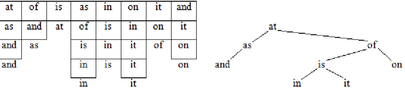
There is another important difference between the traditional Quicksort and the Multikey Quicksort proposed by Bentley et al. In Quicksort, elements link to other elements, making a structure similar to a binary search tree like the one illustrated in Figure 3. However, in the Multikey Quicksort elements are compared character by character, resulting in a ternary search tree like the one illustrated in Figure 4, below.

(24)

As seen, the character by character comparison results in a tree branched in each new character, contrasting with the example of Quicksort, in Figure 3, where the tree is branched by element. This aspect is especially important when comparing strings, because the character by character approach makes it unnecessary to compare all characters between two strings, since it is enough to compare until the first non common character, which most of the times is before the end of one of the strings. This number of positions strictly necessary to compare is called the Longest Common Prefix between two strings, and is explained later in this section.

Bentley et al. [2] first tested the Multikey Quicksort, to which they introduced some enhancements. One of those was partitioning around the median of three elements, resulting in a more balanced tree, which is a simple but effective method of reducing the risk of the worst case to happen. In a performance test they tested the original Multikey Quicksort, against their tuned algorithm and the fastest sorting algorithm at that time. Their tuned Multikey Quicksort showed to be a lot faster than the original algorithm, yet it wasn’t as fast as a highly tuned Radix Sort, which was the fastest algorithm at that time. Even then, in certain contexts, their tuned Multikey Quicksort proved especially suitable, and in those contexts it showed to be even faster than the mentioned Radix Sort.

2.3Quickheap

(25)

Quickheap is a practical and efficient heap for solving the Incremental Sorting problem. It solves the problem in O(n + k log k) time, where n is the size of the array from which we want to get the

smallest k elements [3]. Quickheap is also very fast on the insertions of new elements to the

array, which is a particularly useful feature to this work, and will be covered with more focus later in this dissertation.

Like Quicksort and all other divide and conquer algorithms, Quickheap consists in recursively partitioning the array. The process of dividing a partition into two is done by picking an element, which is called the partitioning pivot. Navarro et al. [3] used the first element of a partition to be its partitioning pivot, so in the example of Figure 3 that is also the procedure, but further in this work some enhancements to the pivot selection criteria will be introduced, such as picking the median of three random selected elements to be the pivot.

Quickheap is intended to sort the array incrementally, which means that it returns one element at a time. The operation of getting only the smallest element of the array is called Quickselect, and

one can say that Quickheap is a sequence of Quickselect calls. To perform those Quickselect

calls, it is required an auxiliary structure, which is used to store the partitioning pivots in such a way that the last added pivot is always on the top position. To perform this way, the best structure to use is a stack, and for the purpose of this dissertation it is frequently mentioned as S.

In the beginning of the Quickheap execution, i.e. before the first Quickselect call is performed,

the stack contains only one element, which is used as a sentinel.

(26)

is especially practical in this work, since such a comparison is done very often and this requires only one if statement to perform the task and avoiding crashes as well.

Creating the stack, adding the sentinel and adding the second sentinel to the array are the first steps when Quickselect is called for the first time. After those initializations, the next operation is

to check the value stored on the top of the stack, and check it against the array. The array is stored in a circular way, so, if on the top of the stack is stored the index of the first element of the array, it is just popped and returned. If the top value points to any other element of the array, then the procedure is different. The array positions between the first and the one pointed by the top of the stack are the partition that will be repartitioned. One element is picked from this partition to be the partitioning pivot (by the median of three elements, as described above). At this point, every element of this partition is compared against the picked pivot, and is either put on its left, if lesser, or on its right, if greater. The pivot is put in the first position after the elements smaller than it, and that position’s index is added to the top of the stack. This procedure is recursively repeated to each newly created partition, until the case in which the element pointed is the first, and immediately popped and returned.

In the end of each recursion of Quickselect the stack is changed: when the top value points to the

first position, the top is popped; if, otherwise, the stack is repartitioned, the new found pivot is added to the top of the stack.

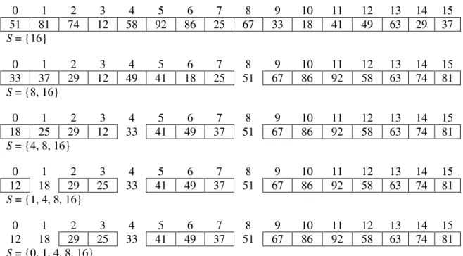
Figure 5, in the next page, shows the first three Quickselect executions of a Quickheap. It shows

(27)

0 1 2 3 4 5 6 7 8 9 10 11 12 13 14 15

51 81 74 12 58 92 86 25 67 33 18 41 49 63 29 37

S = {16}

0 1 2 3 4 5 6 7 8 9 10 11 12 13 14 15

33 37 29 12 49 41 18 25 51 67 86 92 58 63 74 81

S = {8, 16}

0 1 2 3 4 5 6 7 8 9 10 11 12 13 14 15

18 25 29 12 33 41 49 37 51 67 86 92 58 63 74 81

S = {4, 8, 16}

0 1 2 3 4 5 6 7 8 9 10 11 12 13 14 15

12 18 29 25 33 41 49 37 51 67 86 92 58 63 74 81

S = {1, 4, 8, 16}

0 1 2 3 4 5 6 7 8 9 10 11 12 13 14 15

12 18 29 25 33 41 49 37 51 67 86 92 58 63 74 81

S = {0, 1, 4, 8, 16}

Here ends the first Quickselect, returning the smallest element (12). The second Quickselect

drops the last added index from the stack, and gets the next smallest element.

1 2 3 4 5 6 7 8 9 10 11 12 13 14 15

18 29 25 33 41 49 37 51 67 86 92 58 63 74 81

S = {1, 4, 8, 16}

The second Quickselect ends returning the smallest element (18). In the third one the process is

repeated, returning the next smallest value (25) in its end.

2 3 4 5 6 7 8 9 10 11 12 13 14 15

29 25 33 41 49 37 51 67 86 92 58 63 74 81

S = {4, 8, 16}

2 3 4 5 6 7 8 9 10 11 12 13 14 15

25 29 33 41 49 37 51 67 86 92 58 63 74 81

S = {3, 4, 8, 16}

2 3 4 5 6 7 8 9 10 11 12 13 14 15

25 29 33 41 49 37 51 67 86 92 58 63 74 81

S = {2, 3, 4, 8, 16}

(28)

2.3.1 Quickheap Implementation

To implement a Quickheap, four structures are required: an array heap to store the elements; a

stack S to store the indexes of the pivots partitioning the heap; an integer first indicating the first

cell of the heap; and an integer n indicating the size of the heap. These are the data structures

needed to perform the basic operations with the lowest possible complexity.

When creating the Quickheap, the mentioned structures must be initialized. The value of n must

be equal to or greater than the number of elements that will be added to the heap. The array heap

is an array with size equal to n. The auxiliary stack S is a new stack, and at this time it remains

empty. The value of first is initialized with 0. If one wants to create the Quickheap from an array,

then the given array is copied to the array heap and the other attributes are updated. The value of n is the number of elements of the given array, first is the index of the first position of the array.

And the stack S is a new stack, to which is added the index to the n-th position of the array, as a

sentinel value. This operation can be done in time O(1), if the given array is directly used as

heap.

Quickheaps are most used in contexts that require low complexity on getting the minimum element. That’s because Quickheaps are structured in such a way in which this operation performs particularly fast. As described above, and illustrated in Figure 5, every time we obtain the minimum value of the heap it repartitions, taking the smaller elements recursively to the first

positions of the heap, making it faster to get the minimum value. Thus, in cases when the first

element of heap is already a pivot, it is popped and returned, making the complexity O(1).

Otherwise, in the cases in which it is required to repartition the heap, the complexity is, in

average, O(log n), because the problem’s domain is recursively reduced to its half, until the first

position is a pivot.

Following the above approach, if we create a Quickheap from an existing array, and then obtain minimum values from it: we first use the given array as heap, having a complexity O(1), and

(29)

There is another approach to solve the same requirement: if we sequentially insert the elements of the given array to heap, one by one, and in the end obtain the wanted minimum elements from

it. This procedure has a complexity O(log n) for each inserted element, totaling O(n log n) for the

whole process of inserting the elements of the array to the heap. But after that is O(1) for

obtaining each minimum value. Unsurprisingly, the first approach is more effective to solve this example. If we want all the n elements in a sorted order they have the same complexity, but if we

want only some of them, the first approach only orders the heap partially, whereas the second

one orders the whole heap when the insertions are performed. Even then, for the purpose of this

work, the insertion operation is especially attractive, because there will be progressive insertions according to the solution presented in the introduction of this dissertation.

To insert a new element x into heap is required to find the partition where it fits, that means the

pivot limiting that partition in the upside must be greater than x, and the pivot limiting it by the

downside must be smaller than x. To begin with the process of finding that partition, we move

the sentinel (element in the n-th position of heap) one position forward (to the (n+1)-th position),

and put x to the n-th position, which is in the last partition. Then x is compared against the pivot

limiting that partition by the downside, and if the pivot is greater than x they switch positions.

This procedure is repeated until x is greater than a pivot, case in which the process is not

repeated anymore, or x reaches the first position of heap, case in which there are no more pivot

(30)

0 1 2 3 4 5 6 7 8 9 10 11 12 13 14 15 16

18 29 25 33 41 49 37 51 67 86 92 58 63 74 81 ∞ 35

S = {1, 4, 8, 15}

0 1 2 3 4 5 6 7 8 9 10 11 12 13 14 15 16

18 29 25 33 41 49 37 51 67 86 92 58 63 74 81 35 ∞

S = {1, 4, 8, 16}

0 1 2 3 4 5 6 7 8 9 10 11 12 13 14 15 16

18 29 25 33 41 49 37 35 51 86 92 58 63 74 81 67 ∞

S = {1, 4, 9, 16}

Figure 6.Example of inserting a new element in a Quickheap. The new value (35) is compared to the pivots until one smaller than it is found.

Navarro et al. [3] proved that operations upon Quickheaps, such as inserting an element or reorganizing the heap (when obtaining the minimum), cost O(log m) expected amortized time,

where m is the maximum size of the Quickheap. This analysis is based on the observation that

statistically Quickheaps exhibit an exponentially decreasing structure, which means that the pivots form, on average, an exponentially decreasing sequence.

The insertion of new elements in a heap is an especially important operation in the context of this work, because, as mentioned in the introduction of this dissertation, we will build a heap for suffix arrays. Those suffix arrays are going to pop elements to the heap, which are inserted in it.

2.4Suffix Arrays in Secondary Memory

(31)

option, since it is prohibitive because of the spatial constraints that would limit us to work with small texts. The small main memory size makes us think about a good alternative that uses secondary memory.

Up to 2007, the only secondary memory implementations of suffix array construction are so slow that measurements can only be done for small inputs [4]. For that reason, suffix arrays are rarely or never used for processing huge inputs. Instead, less powerful techniques are used, such as having an index of all words appearing in a text. However, using secondary memory to construct suffix arrays has significant potential for improvement, and eventually better techniques and algorithms will appear.

When presenting those algorithms some notation will be used. T always identifies the original

text of which will be built the suffix array, thus T[i] denotes the i-th position of the text T. I will

also frequently mention the term LCP, which means Longest Common Prefix. The LCP is an integer value that denotes the number of characters that two string share from the initial position. For example, the LCP between “Portugal” and “Portuguese” is “Portug”, which has a length of 6 characters. It is frequent to express complexity calculations referring to the LCP value, and there are also some related terms, which we present in Figure 7, bellow. lcp(i, j) denotes the longest

common prefix between SA[i] and SA[j], where SA is the suffix arrays of a text T.

(32)

2.4.1 A Secondary Memory Implementation of Suffix Arrays

Dementiev et al. reviewed [4], in 2008, a set of algorithms that built suffix arrays. They observed that algorithms that only used main memory would be faster than the ones using secondary memory. But since their paper is about secondary memory, they analyzed more deeply the latter ones, concluding that fast secondary memory algorithms that handle large inputs in small amounts of time are yet to appear. The existing ones have high I/O complexity, resulting in unpractical algorithms.

The authors considered that main memory is too expensive for big suffix arrays one may want to build, stating that disk space is two orders of magnitude cheaper than RAM. For that reason they, like us, concluded that it would be a lot worthy to come up with a fast but space-conscious algorithm to build suffix arrays using secondary memory.

In their paper Dementiev et al. presented some techniques that aim to reduce the gap between the main memory and the secondary memory algorithms, and for that purpose they presented some techniques. Those include using a double algorithm, pipelining, and a technique to discard suffixes.

One of the techniques proposed is using a doubling algorithm. The basic idea of this technique is to replace each character of the input by a lexicographic name, which respects the lexicographic order. What makes the technique proposed by Dementiev et al. better than previous secondary memory implementations is that their procedure never actually builds the resulting string of names, rather, it manipulates a sequence P of pairs, where P[i] = (c, i). Each character c is tagged

with its position i in the input. This sequence of pairs is sorted, what makes it easier for scanning

and comparing adjacent tuples, and the process continues as the code chunk in Figure 8 shows. The doubling algorithm proposed computes a suffix array using O(sort(n) ) I/Os

(33)

Figure 8.The Doubling Algorithm and its pipeline representation (as presented by Dementiev et al. [4]).

The pipeline approach proposes that computations in many secondary memory algorithms can be viewed as a data flow through a direct acyclic graph. The authors propose that this graph can be drawn with three types of nodes: file nodes, which represent data that has to be stored physically on disk; streaming nodes, which read a given sequence and output a new sequence using internal buffers; and sorting nodes, which read a sequence and output it in sorted order. The edges of this graph are labeled with the number of machine words flowing between two nodes. The pipeline representation of the Doubling Algorithm is shown in Figure 8, alongside its code.

(34)

that it is possible to implement the Doubling Algorithm using I/Os, which is illustrated in Figure 8.

The authors of this paper also presented a technique to discard suffixes, preventing unnecessary iterations of the algorithm. In the code presented in Figure 8, a lexicographic name is assigned to each suffix, which will not change in posterior iterations. The idea of discarding is to remove tuples considered finished from being analyzed again, thus reducing the work and I/Os in later iterations. It is possible to apply discarding to the presented Doubling Algorithm in two places. In the function name we can take the rank from the previous iteration and add to it the number of

suffixes with the same prefix. The second place is on line (5), where some suffixes can be discarded. As a rule to discard suffixes we need a structure containing the not yet discarded suffixes, marking the ones used in a given iteration. The ones not marked at the end of some iteration can be discarded, since they will not be used in later iteration either.

Dementiev et al. observed that the Doubling Algorithm with discarding can run using I/Os.

The Doubling Algorithm can be generalized to obtain the a-tupling algorithm. For example, if we choose a = 4 we obtain the Quadrupling algorithm, which needs 30% less I/Os than the Doubling

Algorithm. Even then, the authors consider that a = 5 would be the optimal value, but decided to

use a = 4 because 4 is a power of two, making all calculations a lot easier. Besides it is only

(35)

Figure 9.The DC3-algorithm (the 3-tupling algorithm presented by Dementiev et al. [4]).

Given this fact and the techniques presented before, the authors defined a three step algorithm that outlines a linear time algorithm for suffix array construction. The three steps to be followed are: construct the suffix array of the suffixes starting at positions imod 3 ≠ 0; construct the suffix

(36)

Figure 1. The data-flow graph for the DC3-algorithm (as presented by Dementiev et al. [4]).

Dementiev et al. proved that their DC3-algorithm outperforms all previous secondary memory algorithms, since they consider it theoretically optimal and not dependent on the inputs, which are big improvements from previous algorithms. The algorithm proposed is especially useful in this context, since it can be seen as the first practical algorithm able to build suffix arrays. In their tests, this algorithm processed 4GB characters overnight on a low cost machine.

For the purpose of this work, the research done by Dementiev et al. is especially useful, since our goal is also to build suffix arrays using secondary memory. In this context, the DC3-algorithm is a state-of-the-art algorithm to build suffix in secondary memory, providing a good basis for us to compare against our work solution.

2.4.2 Burrow-Wheeler Tranform in Secondary Memory

(37)

obtains the BWT of a text of length n in time and

space (in addition to the text and the BWT itself), for any . Here , where is the length of the shortest unique substring starting at i.

Ferragina et al. [7] recently proposed an algorithm (bwt-disk) that computes the BWT of a text in secondary memory. Their solution uses disk space and can compute the BWT with I/Os and CPU time, where M = and B is

the number of consecutive words in each disk page. Their algorithm makes sequential scans, what lets them take full advantage of modern disk features that make sequential disk access much faster than random accesses, because sequential I/Os are much faster than random I/Os. The authors compared their bwt-disk algorithm against the best current algorithm for computing suffix arrays in external memory, the DC3 algorithm, already covered in this dissertation. Their tests showed that the memory usage reported to both algorithms was similar, although their algorithm showed to run faster than the DC3 algorithm. Furthermore, the bwt-disk algorithm computes the BWT of the text while the DC3 algorithm only computes the suffix array, the additional cost of computing the BWT was ignored.

(38)

3. Our solution

We propose a solution that uses secondary memory to store a significant part of the working data during the construction of the suffix array (and the BWT), so that the main memory usage is much smaller. This makes our algorithm suitable to compute the suffix array of a bigger text in a computer with the same amount of main memory.

For this purpose we divide our algorithm in two parts: the splitting part and the merging part. The splitting part consists in receiving the text, splitting it in several chunks, and outputting a set of suffix arrays, one of each chunk. The merging part is the opposite, it gathers the suffixes from these suffix arrays and merges them into the suffix array of the original text, using a data structure created by us, which is the string heap.

3.1Text Generator

To run our algorithm, we first need a text, which, through this document, we call original text. We created a text generator that generates a random text of size n, from a specific alphabet. This

kind of generation is suitable for debugging and testing specific aspects, such as examples with a lot of branching, which produce a lot of pivots, or others with less dispersion, which produce bigger common prefixes and less pivots.

(39)

3.2Splitting Part

Figure 12.Illustration of the splitting part of our algorithm.

As shown in Figure 11, in the splitting part of our algorithm a text T is divided into k chunks.

From these chunks we obtain k suffix arrays, which are stored in secondary memory.

3.2.1 Partial Suffix Arrays

Given a text T of size n, we divide it into k chunks of size c, i.e. ,

, , .

For each of these text chunks we build the respective suffix array: . We refer to these arrays as partial suffix arrays, since each of them is the suffix array of a chunk of the text T. These arrays are not built in the canonical way, where we assume that there is a $

(40)

3.2.2 Algorithm to Build the Partial Suffix Arrays

To build the partial suffix arrays we use a suffix tree algorithm for each of the k chunks. This

algorithm runs in O(c) time for each chunk and can be processed in parallel.

This algorithm builds the suffix tree for each set of suffixes, and gives the respective suffix array. Since this algorithm builds the suffix tree of the text it is also possible to obtain the LCP between blocks of suffixes inside each partial suffix array, which reduces the time complexity of the merging part of our algorithm.

This procedure uses main memory, which is not a problem since the chunks of the text that originate the partial suffix arrays are relatively small and at this point our program will not use main memory but to build the partial suffix arrays one by one. Thus, the only data stored in main memory in the splitting part of our algorithm is the text and its suffix tree of one of the chunks. Each newly created partial suffix array is stored in secondary memory before the next one is created, each one in a specific file. This way we never fill the main memory with suffixes, in practice only a small part of the suffixes will be stored in main memory alongside the text at each moment.

As we mention through this document, our algorithm has two versions. The first one is a simpler approach to the partial suffix arrays, where each one only contains the indexes of the suffixes (integer values). After building the suffix tree of a given chunk of the text, the algorithm follows its branches and prints its leafs (suffix indexes).

(41)

3.2.3 Blocks of Suffix Indexes

To build the partial suffix arrays in the version with blocks, the suffix tree algorithm doesn’t need to reach the leafs of the suffix tree in order to print the index of a given suffix. Given an LCP value, the algorithm follows the branches up to that value, and then prints all the suffix indexes of that group of branches.

Each block contains 3 data structures:

 An integer number (bkn), representing the number of suffix indexes stored in the block.  An integer number (bklcp), representing the Longest Common Prefix shared by the

elements stored in the block.

 An array (bkar), of size bkn, storing the suffix indexes in this block.

Each block has size (bkn+2), where bkn > 0, i.e. each block contains at least one suffix index.

3.3Merging Part

(42)

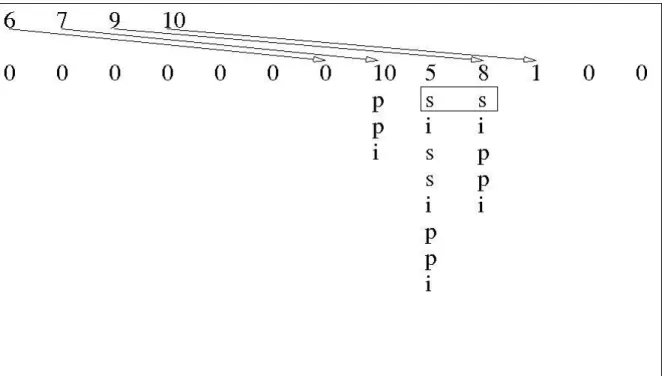
As shown in Figure 12, the merging part of our algorithm consists in receiving values from the partial suffix arrays, gathering them into the heap and successively returning the minimum of the values contained in the heap at each moment. As the heap pops suffixes they are printed to secondary memory, obtaining the suffix array of the text T, or, as Figure 12 illustrates, its

Burrows-Wheeler Transform. The data printed is indifferent in terms of complexity, since the computation of a position of the BWT has time complexity O(1) if we know the respective position of the suffix array, which is the case in our program. As we mentioned in the related work section of this document: BWT [i] = T [SA[i]-1].

Note that all the partial suffix arrays are stored in secondary memory in the beginning of the merging part of our algorithm. Each suffix index stored in there is brought to main memory only when it is pushed into the respective buffer. Once in main memory a suffix remains in the buffer until it is popped to the heap, what happens only at the heap’s request for new elements from that specific buffer. It remains in the heap as long as it is not the smallest suffix in there. In that moment it is printed to the BWT file, thus again to secondary memory.

3.3.1 Buffers

Each of the described partial suffix arrays has a buffer that stores the suffix indexes in main memory. Despite being in main memory, those indexes are still out of the heap, and are popped into it only when needed.

(43)

As mentioned above, the buffers can receive suffix indexes alone or in blocks. In the first approach the buffers get the suffixes one by one, and pop them to the heap in the same order. In the second approach, despite storing blocks the procedure is similar, the buffers receive the blocks from the partial suffix arrays, and pop them into the heap in the same order they received them.

Each buffer has a counter that tells how many suffix indexes from the respective partial suffix array are yet to be passed to the heap. When a counter reaches zero all the suffix indexes for which that buffer was responsible for were already popped to the heap, meaning that the buffer has no more work to do in that execution.

3.3.2 String Heap

The particular heap structure that we use is based on the Quickheap proposed by Navarro, et al. [3], which is a hierarchical algorithm, inspired on the Quicksort algorithm. We also use a technique proposed by Bentley, et al. [2], who pointed out that using ternary Quicksort was better than using the original binary Quicksort, for building suffix arrays. We use both studies in our work, particularly to make our heap. The main idea is to have a heap similar to the one presented by Navarro, et al., but introducing the enhancement based on the observation of Bentley, et al., which is: ternary searches perform better than binary searches to compare suffixes.

Being ternary means that each partitioning produces three partitions. These are: the group of elements whose first character is lesser than the first character of the pivot; the group of elements whose first character is equal to the one of the pivot; and the group of the ones with a greater first character comparing with the one of the pivot. All the comparison operations are always performed character by character, meaning that the comparison between two suffixes end as soon a different character is found.

(44)

reduces the average time complexity of the insertion operation from to

, where n is the size of the text and is the average LCP between the text suffixes. This

enhancement avoids the need to compare all the characters up to the LCP value, is accumulative, thus each compared character is valid not only for one suffix but for all that share that character with it.

Using this approach on a character by character partitioning system is especially relevant because we are working with strings, reason why we call this structure a String Heap.

The heap is internally divided in partitions, as in the Quickheap presented in the related work section of this document. Each partition is a group of contiguous positions of the heap, whose elements share a common LCP (x). One of those elements is the pivot of the partition, and its

first x characters represent the first x characters of any other suffix in the partition. The pivots

define frontiers between partitions, since a partition’s pivot is its last position

3.3.3 Input/Output Operations

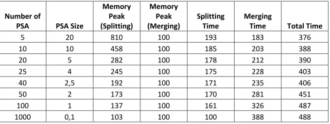
The way the suffixes are popped from secondary memory to main memory is a crucial issue raised in the implementation of the algorithm. To better answer this question we need to take three factors into account: the number of partial suffix arrays, the size of each buffer, and the number of elements popped from secondary memory to the buffers on each read.

(45)

For the correctness of our algorithm’s results the heap must always contain at least one element from each partial suffix array, meaning that no counter can reach zero, except either in the beginning of the execution or when its buffer is empty, i.e. passed all the elements from its partial suffix array to the heap. Whenever the heap runs out of elements from any of the partial suffix arrays the execution stops.

In the beginning of the execution the heap asks for suffixes from all the partial suffix arrays, until it contains at least one from each of them. Yet as the heap pops values it redefines that policy, and will tend to ask for values rather to the suffix arrays where those values belonged, aiming to maintain a balanced number of elements of each suffix array. Note that the I/Os take longer to bring new suffixes to the heap than the heap takes to return results, since a main memory read is much faster than a disk read. Because of this fact the heap tends to pop results at a faster pace than it receives, thus, for the reason mentioned above, it tends to block waiting for new suffixes to be pushed. To mitigate the effects of this issue we need to decrease as much as we can the number of times it blocks.

Being popped from suffix arrays of parts of the text, we know that each element obtained by the heap is smaller than any other that will ever come from the same partial suffix array, still it can be greater than the values in the other partial suffix arrays. This is why the heap always needs to contain at least one element from each partial suffix array, otherwise there would be no guarantee that the suffixes from the missing buffers weren’t smaller than the suffixes in the heap. For this reason, if at any time the heap contains no elements from a given buffer, and for some reason the heap is unable to obtain elements from it, the execution has to stop, because there is no guarantee that the heap is able to pop the minimum value from all the elements that are yet to be returned. If such a situation occurs, it is mandatory that the execution blocks, otherwise we can’t guarantee the correctness.

(46)

When deciding the best policy to adopt to prevent the heap from blocking we need to consider some tradeoffs. The heap must contain elements from all the non empty partial suffix arrays, otherwise the execution will block. To avoid this problem we could bring a new element to the heap every time one is popped from it, yet such a policy would represent too many I/Os. We could also flood the heap with many values from each buffer, but too many values in the heap means exaggerated main memory consumption. The policy we choose must reflect all these concerns, trying to manage these problems.

The factors we need to pay attention when making such a decision are the number of partial suffix arrays in which we divide the text, the size of each buffer, and the number of elements in the heap. The more partial suffix arrays we have the less suffixes each one contains; conversely, the less partial suffix arrays we have, the more elements each partial suffix array will contain. Each of these situations has an outcome. If we have more partial suffix arrays their counters in the heap tend to have smaller values, which means that the heap will ask for new suffixes more often.

If each partial suffix array contains less elements means, in the case of blocks of suffixes, that the blocks are smaller, not taking full advantage from having the suffixes grouped in blocks by their LCP. On the other hand, if we have less partial suffix arrays we get much more from that fact, since the blocks will be bigger, requiring less processing in the heap. However, popping those bigger blocks to the heap means more main memory consumption.

We also need to decide the number of suffix indexes that are pushed into main memory on each read to the buffers. The more elements read on each operation, the less impact I/Os have on its execution, however, if the buffers store too many suffixes that can represent too much main memory consumption.

(47)

4. Algorithm Implementation

4.1Initial Parameters

Before running our algorithm we need to set the following parameters:

 Size of the input text (n). The number of characters of the text given as input.

 Size of the heap (m). The maximum number of suffixes the heap can contain at a time.  Size of each partial suffix array (c). The size of each chunk of the text from which the

partial suffix arrays are obtained.

 Size of each buffer (d). The maximum number of suffixes a buffer can contain at a time.  LCP to build the blocks (bklcp). The size of the prefix that the suffixes inside the partial

suffix array must share to belong to a common block. This parameter is needed only if we are running the version that uses blocks of suffix indexes.

Note that the number of partial suffix arrays (k) is also a fundamental parameter for the execution

of our algorithm, however we don’t need to set it manually. Having the size of the text (n) and

the size of each partial suffix array (c) our program calculates it in the beginning of its execution.

4.2Splitter

The splitter divides the text into k chunks, each of them with size c. For each chunk it builds the

respective suffix tree, and follows its branches to obtain the c suffixes one by one. For each

partial suffix array the splitter creates a new file, and each suffix is written to it once it is obtained. If we want to store blocks instead of single suffixes the branches of the suffix tree are followed until an LCP of at least bklcp is reached, moment when a new block is created with the

(48)

Note that the suffixes obtained with the suffix tree have indexes in the context of that chunk, however, before storing them in the partial suffix arrays they are added the number of suffixes stored in the previous suffix arrays. Thus, the indexes stored in the files are global indexes, instead of partial, even though they are stored in partial suffix arrays.

4.3Merger

4.3.1 Data Structures

The merger consists in two types of structures: heap and buffers. We have one heap and k

buffers, one for each partial suffix array. The buffers feed the heap with elements, and the heap sorts the elements and pops them into the final suffix array, which we use to create the Burrows-Wheeler Transform of the text.

Therefore the merging part of our algorithm begins with the creation of the heap and initialization of its data structures. The heap contains two structures that maintain the data related to the buffers, we also created a type Buffer to better distribute the tasks involved in this part of

the algorithm.

 Buffer– A data structure created by us that contains:

o _file – A permanent reference to the file where the respective partial suffix array is stored.

o _ar– An array storing the indexes of the suffixes it contains at each moment. o _elemsleft – An integer counting down the elements left to return from its

respective partial suffix array. Note that each buffer will never contain all the elements in its respective partial suffix array (c), thus it has a smaller capacity (d)

and is used as a circular array.

 bufs – An array of elements of type Buffer, to store pointers to the buffers where the

(49)

 bufcount– An array of integers to store the number of elements from each buffer that are

in the heap at each moment. Note that each position of this array counts the elements of the buffer pointed by the same position in the array bufs.

The heap also has data structures whose purpose is to maintain its internal operations:

 ar– An array of integers to store the indexes of the suffixes in the heap at each moment.

This array has size m+2, i.e. the maximum number of elements that the heap can contain

at each time plus the two sentinels. Note that this is a circular array, thus its size (m) can

be much smaller than the total number of suffixes (n).

 pvts– An array of integers that stores the pivots. Each of the integer numbers stored is the

position of a pivot, i.e. if a value i is in the array pvts the element ar[i] is a pivot.

 lcps – An array of integers that stores the value of the LCP in each partition of ar. Each

position of this array corresponds to the same position in the array pvts, i.e. lcps[i]

contains the value of the Longest Common Prefix between ar[pvts[i]] and any other

element of the partition in which it is the upper limit and ar[pvts[i+1]] is the lower limit.

Note that we define that even though ar[pvts[i]] belongs to this partition ar[pvts[i+1]]

does not, therefore the LCP value lcps[i] is not valid between the lower limit and any

element of the partition.

 bplcps– An array of integers that stores the value of the LCP between each pair of pivots.

Each position of this array also corresponds to the same position in the array pvts, i.e. bplcps[i] contains the value of the LCP between ar[pvts[i]] and ar[pvts[i+1]]. Note that

(50)

 i – An integer value with the position of the last pivot in the array ar. This pivot is the

smallest element in the heap, thus the next to return.

Note that the order of the pivots in pvts is inverse to the order of the suffixes in ar. The array pvts

has decreasing order, i.e. pvts[i] contains a bigger value that pvts[i+1], apart from sentinels. In

the cases that the heap rotates this is not absolutely true, since pvts[i+1] can be bigger than pvts[i], however the order is the same and pvts[i+1] is always closer to the smaller sentinel than pvts[i].

As we mentioned in the related work section, the pivots array (pvts) is a stack, thus we

implemented it this way because it is more time efficient than implementing it in the same order than the heap. This fact is explained in the next section, mainly in the insertion and extraction operations, in the heap.

In both arrays ar and pvts we use sentinels to avoid making conditions to catch the case when the

index gets out of the valid positions, and yet preventing the program to crash. In both cases the sentinels are located in the position before the first and after the last valid position, the small and large sentinels, respectively.

4.3.2 Operations

The type Buffer is used to store elements and, when the heap asks, pop them into there. Its

operations are:

 Initialization – For the array ar it allocates d positions in memory. The integer elemsleft is

initialized with the value c, since in the beginning of the execution all elements from the

(51)

 next– This function is responsible for returning the next suffix index to the heap. In the

case we are using blocks of suffixes it returns the next block of suffix indexes.

In the heap these are the basic operations. The remaining are presented in the next sub-section.  Initialization

o _ar – This array uses O(_m) space, which is allocated in the beginning of the execution of the algorithm.

o _pvts – This array uses O(log _m) space on average, which is allocated in the initialization.

o _lcpsand _bplcps– Being analog to _pvts each of these arrays also use O(log _m), and both are allocated in the beginning as well.

 check_buffer– This function receives the buffer index (b), and checks if bufcount[b] > 0.

If not, that means the heap has run out of suffixes from the buffer b, therefore at least one

new suffix needs to be inserted from that buffer.

 Comparison function – This function is used in every comparison between suffixes inside the heap. It receives the indexes of the two suffixes to compare (A and B) and compares only the character in the position given. This function returns a value: 0 if T[A] is equal

to T[B]; negative if T[B] is greater than T[A]; and positive if T[A] is greater than T[B]. If

(52)

4.3.3 Heap Insertion

This function is used to insert new suffixes in the heap, thus it receives the index (b) of the buffer

where to obtain those. The insertion begins with evoking the function next of the buffer stored in bufs[b], obtaining the suffix suf. This suffix is compared with all the pivots, one by one. For each

pivot pvts[i] the maximum number of characters compared is lcps[i], i.e. comparing the

characters until the LCP of the partition is enough to decide if suf needs to be compared with the

next pivot.

Since we know the LCP in each partition and the LCP between each pair of pivots, we use those values in the insertion of new elements:

 bplcps– The LCP between pivots are very important to reduce the execution time of our

algorithm, by reducing the number of characters that need to be compared on each insertion. Once the new suffix (suf) is compared with one pivot, pvts[i], the LCP between

them (lcp) is stored, and in the cases when lcp > 0 and bplcps[i] > 0 there is a number of

characters that does not need to be compared again, i.e. min(lcp, bplcps[i]) is that

number, where min is a function that returns the minimum of two numbers.

 lcps– The LCP of a partition is used when we need to decide if the new suffix is inserted

in an existing partition or if it needs to be set as a new pivot. It can be inserted in a partition if, and only if, the LCP between suf and the pivot that is the upper limit of the

partition, lcp, is at least equal to the partition LCP, lcps[i], i.e. lcp >= lcps[i]. This is

essential to maintain the correctness of the heap.

The insertion function runs two different loops, one inside the other. Each iteration of the outer loop means a new pivot compared against the new suffix. Each iteration of the inner loop means a new character compared between the current pivot and suf.

As mentioned, we don’t need to compare more characters than the LCP of the current partition, thus one of the conditions to break the inner loop is that, if lcp = lcps[i]. The other condition is

(53)

current characters of suf and the pivot is not zero, i.e. if the character is different then suf is

different than the pivot, before the LCP.

Once the inner loop is broken the outer one is also broken if, and only if, suf is greater than the

compared pivot, i.e. if the inner loop didn’t exhaust the partition LCP, and at some character the comparison returned that the pivot’s character is smaller than the new suffix’s one. According to other conditions, the new suffix can be inserted into the heap in two different ways:

 The new suffix is inserted in the partition between ar[pvts[i]] and ar[pvts[i-1]] – This

case happens if, and only if, the LCP between the previously compared pivot, pvts[i-1],

and suf is at least equal to the partition’s, i.e. LCP(pvts[i-1], suf) >= lcps[i-1].

 The new element becomes a new pivot between ar[pvts[i]] and ar[pvts[i-1]] – This case

happens if the LCP between previously compared pivot, pvts[i-1], and suf is smaller than

the partition’s, i.e. LCP(pvts[i-1], suf) < lcps[i-1]. In this case the pivots are put one

position ahead, i.e. pvts[j] becomes pvts[j+1] for every j >= i, and pvts[i] = suf, to avoid

unnecessary character comparisons in the next insertions, bplcps[i] is set with the value

LCP(pvts[i], suf), i.e. the LCP between the newly created pivot and the next one.

Whenever a new suffix is inserted into the heap, the counter of elements from the buffer it came from is incremented by one unit, i.e. bufcount[b] = bufcount[b]+1. If instead of one single suffix

a block of suffixes is inserted, then the counter is incremented by as many units as the size of the block.

The insertion of a new suffix into the heap runs in time on average, where p is the