Abstract—To more fully utilize the potential offered by multi-core processors, programming languages must have features for expressing parallelism. One promising approach is collection-oriented operations, which are easily expressed by the programmer and can be implemented by the runtime system in a parallel fashion for improved performance. However, the ordinary implementation requires a barrier synchronization among all the processors after each parallel operation, thereby creating a performance penalty that grows with the number of processors. For large numbers of processors, this inhibits scalability and reduces performance especially for smaller size data sets. This paper explores a optimization technique called operator fusion, which removes the necessity for barrier synchronization. The general principles and rules governing the use of operator fusion are described and then illustrated with a specific collection-oriented parallel library that we have developed for the object-oriented programming language Scala, which is an extension of the language Java. Performance improvement resulting from operator fusion is analyzed for several benchmark programs on a computer with a multi-core processor.
Index Terms— data parallel, multi-core processor, parallel programming, Scala
I. INTRODUCTION
O help the programmer specify parallelism in a program, the programming language must have some special parallel programming features. The predominant approach used so far is multi-threading, in which the programmer explicitly assigns computing tasks to individual parallel threads. If the parallel threads modify shared data, then locking is used to provide atomic access. This approach has several drawbacks. The programmer is involved in many of the low-level details of management and synchronization of parallel tasks. Also, multi-threaded programs have potential data races that essentially create a nondeterministic program: a program that may produce different outputs for the same input data during different executions. Program deadlocks may also occur in a nondeterministic fashion. This nondeterminism complicates the software development process, and makes it more difficult to develop reliable software.
One promising approach to solve many of these problems is high-level collection-oriented operations, in which every element of the collection is operated upon in parallel by the same operation. This is often called data parallel programming. One example is the array operations of the language Fortran 90 [1], which may have a sequential or
Manuscript received August 15, 2011; revised November 14, 2011. Bruce P. Lester is Professor, Computer Science Department, Maharishi University of Management, Fairfield, Iowa 52556 USA (e-mail: [email protected]).
parallel implementation. A more sophisticated set of operations is found in High-Performance Fortran [2, 3], including data distribution directives and user-defined data parallel functions. The widely publicized MapReduce [4] operation used by Google is another example of a collection-oriented parallel operation.
One of the earliest commercial applications of data parallel programming during the late 1980s was in the Connection Machine [5] of Thinking Machines Corporation. The programming languages available for the Connection Machine included data parallel versions of both Lisp and C. Much of what was known at that time about data parallel programming is summarized in the book by Guy Blelloch, Vector Models for Data-Parallel Computing [6]. Looking back even earlier, the array operations of the language APL [7] can be considered as primitive examples of collection-oriented operations that can have a data parallel implementation. In the case of APL, the array operations were not introduced for the purpose of parallel execution, but simply to make the programming process easier by providing higher level programming abstractions.
More recent examples of data parallel languages include Ct [8], a language under development by Intel for their experimental terascale processor architectures. The company RapidMind has successfully marketed a data parallel extension of the C++ language with collective operations on arrays [9]. Intel has just released a software package called Array Building Blocks [10] that combines and extends many of the features of Ct and the RapidMind extensions. Researchers at Stanford University have developed a data parallel extension of the C language called Brook [11], intended for efficient execution on computers with GPU coprocessors. Brook allows user-defined data-parallel functions on streams, which are essentially large data arrays. The language X10 under development by IBM [12] and HPJava [13] are both data parallel versions of Java, intended for scientific and engineering applications on high-performance computer clusters.
II. OPERATOR FUSION
One of the main performance issues in data parallel programming is the need for synchronizing the processors after each data parallel operation. Data parallel operations are more widely applicable for general purpose programming if they are fairly primitive in nature. Then the programmer can construct a parallel program by combining large numbers of these primitive operations. However, the barrier synchronization required after each data parallel operation creates a performance penalty, which grows with the number of processors. For large numbers of processors, this inhibits scalability and reduces performance especially
Operator Fusion in a Data Parallel Library
Bruce P. Lester
for smaller size data sets.
In this paper, we explore a technique called operator fusion, which removes the necessity for barrier synchronization after each data parallel operation. Data parallel operations are implemented by dividing the work among the available processors. To be sure that the operation is complete, all of the processors execute a barrier before moving on to the next operation. However, under certain circumstances, it is possible for a processor to move immediately to the next data parallel operation without waiting for the other processors. For example, consider a sequence of four data parallel operations: P, Q, R, S. In an ordinary parallel implementation, all processors are required to finish their assigned portion of the computing for operation P, and then execute a barrier before any can begin on operation Q. Similarly, all processors must finish their work on operation Q before beginning R. With an implementation based on operator fusion, a processor completes its work on data parallel operation P and then moves on to operation Q immediately; similarly for operations R and S. Thus, the sequence of four data parallel operations can be executed with only one barrier operation after S, instead of four barriers in the implementation without operator fusion.
In this paper, we explore the use of operator fusion in a collection-oriented parallel library. The library is an add-on to an ordinary object-oriented programming language. The library implementation is done completely at runtime. In section III we present the general principles underlying the operator fusion optimization, including a general algorithm for determining when it can be used. In subsequent sections, we describe our collection-oriented library and analyze the performance improvement resulting from operator fusion for several benchmark programs.
Removing processor synchronization barriers to improve performance of parallel programs is not a new idea. Some parallel programming languages have explicit instructions that the programmer can use to indicate a barrier is not necessary in certain circumstances. For example, the language OpenMP allows a NOWAIT directive to prevent a barrier synchronization among the threads executing a parallel loop. In contrast to this, we are concerned with automatic operator fusion, done completely at runtime by the collection-oriented library without any knowledge or intervention by the programmer.
The Intel Array Building Blocks (ArBB) library for C++ does include some automatic operator fusion. However, this optimization is applied only in the limited context of function bodies that are invoked with a special ArBB call operation. Furthermore, all of the ordinary C++ flow of control instructions (for, while, if) in the function body must be replaced by special ArBB flow of control operations. In contrast to this, our implementation of operator fusion is automatically applied to every individual collection-oriented operation in the library at runtime.
This paper is a revised and extended version of an earlier paper by Lester [14], and includes significantly more details about the sample data parallel library (section IV) and its implementation (section VI). These additional details greatly enrich the general discussion and analysis of operator fusion.
III. GENERAL PRINCIPLES
The first step is to explore the general principles of operator fusion and develop a simple algorithm for determining when operator fusion is possible. For this purpose, consider a very general framework with a User Program written in any high-level language. Embedded at various points in this User Program are calls to data parallel operations. These calls may be features of the programming language, or simply calls to library functions (methods). To allow the possibility of operator fusion of the data parallel operations, two simple assumptions are needed: isolation and partitioning. These will be explored in the next two subsections.
A. Isolation of Data Parallel Operations
The first assumption is the existence of a clean interface between the User Program and the data parallel operations. The data parallel operations perform transformations on a special group of collections (data structures), which we call Data Parallel Collections (abbreviated: DP-Collections). The User Program interacts with the DP-Collections through a fixed set of Data Parallel Operations (abbreviated: DP -Operations). The User Program passes parameters to these DP-Operations, which are used to carry data into the operations and return data back to the User Program. However, the User Program has no direct access to the DP-Collections, except via one of these special DP-Operations. Furthermore, the DP-Operations have no side-effects: they can only read/write the DP-Collections and the data passed as parameters from the User Program. In other words, the DP-Operations are isolated from the User Program data, and similarly the User Program is isolated from the DP-Collections.
This isolation assumption is very reasonable and will probably be valid for a wide range of data parallel libraries, beyond the specific data parallel library described in subsequent sections of this paper. For example, the Intel Ct library [8] and Array Building Blocks library [10] both satisfy the isolation property. For now, let us determine to what extent operator fusion of data parallel operations is possible based only on this simple isolation assumption. For this purpose, a useful analytical tool is a History Graph of the DP-Operations. During each specific execution of the User Program, a series of DP-Operations (d1, d2, …, dn) will
be generated. Each DP-Operation di will have parameters,
some of which may be a reference to a specific DP-Collection, and some of which may be a reference to a User Program data value (object). The execution history of the DP-Operations defines a directed, acyclic graph as follows:
Each executed DP-Operation di is a node in the
graph. The index i is called the sequence number or timestamp of the operation.
Each DP-Collection referenced by a parameter of any DP-Operation is a node in the graph.
If DP-Collection c is read by DP-Operation di , there
is an edge from c to di. If c is modified by di , there
is an edge from di to c.
If User Program data value u is read by DP-Operation di , there is an edge from u to di. If u is
modified by di , there is an edge from di to u.
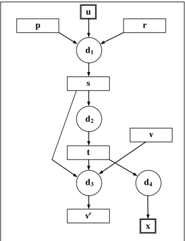
An example of a History Graph is shown in Fig. 1. The particular sequence of DP-Operations (d1, d2, d3, d4) in the
history is generated by the User Program, depending on the input data. We are not suggesting that such a History Graph actually be constructed during the execution of a real program. We are just using the graph as a conceptual tool to help analyze and understand the principles of operator fusion. Each DP-Operation in the graph is executed by a team of Worker Threads running in parallel. Now consider the following question: under what conditions can the barrier synchronization after each DP-Operation be safely removed?
For any given DP-Operation operation di in the graph with
an input DP-Collection v, let I(di, v, m) denote the set of data
elements in DP-Collection v that are directly read by Worker Thread m during DP-Operation di. For DP-Operation dj with
an output DP-Collection v, let O(dj, v, k) denote the set of
data elements in DP-Collection v that are directly written by Worker Thread k during DP-Operation dj.
A data element e of a DP-Collection v is said to be a cross-thread data element if there exist DP-Operations di
and dj, such that eϵ O(dj, v, k) and eϵ I(di, v, m) and km.
In simple words, a cross-thread data element is one that is created (written) by one Worker Thread and then consumed (read) by a different Worker Thread. Cross-thread data items restrict the possibilities for operator fusion of the DP-Operations. If Worker Thread k writes a cross-thread data item e during DP-Operation operation dj, and e is read by a
different Worker Thread m during a subsequent DP-Operation operation di, then some kind of barrier
synchronization among the Worker Threads is required after operation dj. Otherwise, Worker m might attempt to read
data item e before it is created by Worker k.
If the output DP-Collection v of any DP-Operation operation di in the history graph has no cross-thread data
items, then no barrier synchronization is required after operation di. Thus, all the Worker Threads involved in the
execution of operation di can immediately move on to the
next DP-Operation operation dj as soon as they complete
their share of operation di. Thus, each Worker Thread
experiences a fusion of its computing on operations di and dj.
The general discussion of the last few paragraphs has assumed that the output of the Operation is a DP-Collection. However, some DP-Operations may produce an output data value (object) that is not a DP-Collection. As an example, consider operation d4 and its output x in Fig. 1. A
reference to this object x is returned to the User Program by operation d4. Since x is not a DP-Collection, the User
Program may directly access the data of x. Thus, it is necessary to make sure the Worker Threads have completed their computation of x before returning to the User Program after the call to operation d4. Thus, barrier synchronization is
required after operation d4 that includes all the Worker
Threads and also the Master Thread executing the User Program. When the Master Thread is included, we call it a Strong Barrier. However, as long as the output of any DP-Operation is a DP-Collection, then a strong barrier is not necessary.
The situation is similar for an input parameter to a DP-Operation that is not a DP-Collection, for example input u to DP-Operation d1 in Fig. 1. The User Program may have
another reference to data value (object) u and attempt to modify it. Therefore, d1 must complete its work before the
User Program is allowed to continue. Thus, a strong barrier is needed after d1, unless u is an immutable object, which
cannot be modified.
B. Partitioning of Data Parallel Collections
The above general discussion of operator fusion is based completely on the assumption of isolation between the User Program and DP-Collections. Now one additional assumption will allow the development of a simple and practical operator fusion algorithm: each DP-Collection has a standard (default) partitioning. The partitions are disjoint and cover the whole DP-Collection. The overall purpose of the partitioning is to facilitate data parallelism. Each Worker Thread can be assigned to work on a different partition in parallel with no interference.
Partitioning facilitates operator fusion if the same partitioning is used by many different DP-Operations. For example, consider a DP-Collection v with partitions p1, p2,
…, pm. Now assume that Worker Threads W1, W2, …, Wm
are assigned to work on these partitions independently in parallel during a particular DP-Operation di. If the same
group of m Worker Threads is assigned to the partitions in the same way during the subsequent DP-Operations di+1,
p
r
s
v
t
v
x
d
1d2
d
3d
4Figure 1. History Graph of PVector Operations.
then there is no need for a barrier after di — fusion of
operations di and di+1 is possible without introducing any
data races or timing-dependent errors. After completing its share of the computing in operation di, Worker k can move
on immediately to operation di+1 without waiting for the
other Workers — there is no need for a barrier after operation di. Using the terminology of the previous section,
the standard partitioning prevents the possibility of any cross-thread data elements in this particular DP-Collection v.
At this stage of analysis, we are not specifying any details about the nature of the data structures allowed in the DP-Collections or the particular partitioning method. We only assume there is some standard partitioning method for each DP-Collection. If this standard partitioning is used by many of the DP-Operations for allocating Worker Threads, then there will be a lot of opportunity for fusion of the DP-Operations. However, all DP-Operations are not required to adhere to the standard partitioning. Some DP-Operation may use a different partitioning or may not have any distinct partitioning at all, in which case these DP-Operations will not be candidates for operator fusion.
This assumption of a standard (default) partitioning for each DP-Collection, along with the isolation assumption from Section IIIA, will allow us to develop a simple operator fusionalgorithm to determine whether specific DP-Operations require a barrier synchronization or not. The input to this algorithm will be a descriptor for each DP-Operation that specifies certain important properties of that operation.
Each DP-Operation d has one or more input parameters, some of which may be DP-Collections, and an output parameter which may be a DP-Collection (see the History Graph of Fig. 1 for examples). For each of these DP-Collection parameters, the operator fusion algorithm needs to know whether or not DP-Operation d adheres to the standard partitioning of that DP-Collection. If the standard partitioning of any input parameter is violated, this is called an input crossing; similarly, violation for an output parameter is called an outputcrossing.
C. The Operator Fusion Algorithm
Following is summary of the seven properties of each DP-Operation that will serve as input to the operator fusion algorithm:
InputCross: true if this operation has an input crossing
OutputCross: true if this operation has an output crossing
OutDP: true if the output of this operation is a DP-Collection
InUserData: true if any of the inputs to this operation is not a DP-Collection
OutputNew: true is the output of this operation is a newly created DP-Collection
HasBarrier: true if this operation has an internal barrier synchronization of the Worker Threads
HasStrongBarrier: true if this operation has an internal strong barrier synchronization
These seven properties are static – they only need to be determined once for each DP-Operation in the library. The properties do not depend on the particular User Program, but only on the definition of the DP-Operations and the particular implementation of the operations.
In addition to the above static information, the operator fusion algorithm also needs some dynamic information that must be gathered during the execution of the User Program. Each call to any DP-Operation by the User Program is assigned a unique sequencenumber, which serves as a kind of time stamp. Each DP-Collection also has a unique time stamp: the sequence number of the DP-Operation that created it. This is assigned dynamically when the DP-Collection is created. Also, each specific DP-DP-Collection has a time stamp (sequence number) of the most recent DP-Operation to perform an input crossing on it (InCrossTime). One additional piece of dynamic information required is the time stamp of the most recent barrier operation.
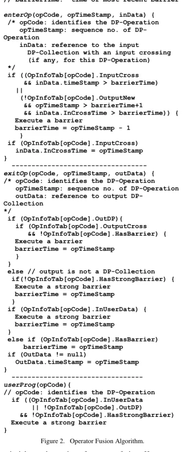
The operator fusion algorithm is shown in Fig. 2 and has there separate procedures. enterOp is called by each Worker Thread before beginning each DP-Operation to determine whether a barrier is needed before execution of the DP-Operation. exitOp is called by each Worker Thread after each DP-Operation is complete to determine whether a barrier is needed before moving on to the next DP-Operation. userProg is called by the User Program after each DP-Operation call to determine whether the User Program must participate in a strong barrier with the Worker Threads before continuing.
All three procedures in this operator fusion algorithm depend heavily on the properties of the DP-Operations, which is contained in the array OpInfoTab. For example, OpInfoTab[opcode].InputCross is true if the DP-Operation identified by opcode has an input crossing on one of its DP-Collection input parameters. The algorithm also uses the time stamps of the Operations and the DP-Collections. The variable barrierTime, which is the time stamp of the most recent barrier, is used and modified during the algorithm. The procedures of this algorithm have no loops and can therefore be executed in constant time.
The focus of this operator fusion algorithm is to detect those specific conditions that require a barrier operation, and avoid a barrier whenever possible. The algorithm is quite general and is based only the two assumptions described earlier: isolation and partitioning. The implementation dependent aspects of the algorithm are captured by the seven properties of the DP-Operations as found in the array OpInfoTab.
Now we will apply this operator fusion algorithm to a specific collection-oriented parallel library for the language Scala. The subsequent sections of this paper describe the library in detail and give an example program that uses the library to solve a partial differential equation. We also summarize the results of performance studies on several benchmark programs showing that operator fusion significantly improves the performance of the library.
IV. DATA PARALLEL LIBRARY
principles and practice of operator fusion. However, to illustrate the principles and show that the technique is practical, it is necessary to focus on a specific implementation. For this purpose, we use a collection-oriented parallel library for the object-collection-oriented language Scala, which extends the language Java by adding functional programming features. Scala is compiled into Java byte-code and is executed by the Java Virtual Machine. Any of the Java library functions may be called from within a Scala
program. We chose Scala [15] as our implementation language because it is particularly well suited for creating runtime libraries. However, the collection-oriented parallel library presented in this paper could also be implemented with operator fusion in Java, C#, or any object-oriented language. Runtime operator fusion in data parallel libraries is in no way limited to the language Scala.
The basic parallel collection object we use in our library is called a ParallelVector (abbreviated PVector). A Parallel Vector is an indexed sequence of data items, which bears some resemblance to a one-dimensional array. However, the range of operations available for Parallel Vectors is really quite different from a simple array, as described in the subsequent sections of this paper. Parallel Vectors are implemented in Scala with a generic library class
PVector[T]. To create an instance of PVector in a Scala
program, one must supply a specific type (or arbitrary class name) for the generic type [T].
The PVector class in our data parallel Scala library provides several constructors for creating and populating new PVector objects. The PVector class also has a variety of methods that can be invoked by the user program to transform and/or combine PVector objects. The calls to the PVector constructors and methods are imbedded in the user program. The implementation of the constructors and methods is done completely within the library using parallelism. Thus, the parallelism is essentially hidden from the user program. The user does not have to deal with the complexities and problems associated with parallel program-ming, as briefly described in the Introductory section of this paper.
The fusion of the PVector operations is also contained within the library implementation, and is therefore hidden from the user program. Thus, the user may view the PVector as just another type of collection with a set of available operations implemented in the library. Using the terminology of section III, the PVectors are the DP-Collections, and PVector methods are the DP-Operations.
Our data parallel Scala library currently implements a total of fifteen primitive operations on PVectors. For purposes of understanding, these can be divided into five major categories: Map, Reduce, Permute, Initialize, Input/Output. Following is a brief description of the operations contained in each of these categories. This discussion uses some Scala code segments. Readers unfamiliar with Scala may refer to [15] or any of the online Scala tutorials that are easily found on the internet. However, the Scala syntax is so similar to Java that it should be understandable by any reader who has some familiarity with Java or C#.
A. Map Operations
The map operation is a very powerful data parallel operation that applies a user-defined function to each element of a PVector. The abstract execution model for this application is a virtual processor operating in parallel at each element of the PVector. In practice, this may be implemented in the library using a combination of parallel and sequential execution. The signature of the map method is as follows:
// OpInfoTab: properties of DP-Operations // barrierTime: time of most recent barrier
enterOp(opCode, opTimeStamp, inData) { /* opCode: identifies the DP-Operation opTimeStamp: sequence no. of DP-Operation
inData: reference to the input
DP-Collection with an input crossing (if any, for this DP-Operation) */
if ((OpInfoTab[opCode].InputCross && inData.timeStamp > barrierTime) ||
(!OpInfoTab[opCode].OutputNew && opTimeStamp > barrierTime+1
&& inData.InCrossTime > barrierTime)) { Execute a barrier
barrierTime = opTimeStamp - 1 }
if (OpInfoTab[opCode].InputCross) inData.InCrossTime = opTimeStamp }
--- exitOp(opCode, opTimeStamp, outData) { /* opCode: identifies the DP-Operation opTimeStamp: sequence no. of DP-Operation outData: reference to output
DP-Collection */
if (OpInfoTab[opCode].OutDP){
if (OpInfoTab[opCode].OutputCross && !OpInfoTab[opCode].HasBarrier) { Execute a barrier
barrierTime = opTimeStamp }
}
else // output is not a DP-Collection if(!OpInfoTab[opCode].HasStrongBarrier) { Execute a strong barrier
barrierTime = opTimeStamp }
if (OpInfoTab[opCode].InUserData) { Execute a strong barrier
barrierTime = opTimeStamp }
else if (OpInfoTab[opCode].HasBarrier) barrierTime = opTimeStamp
if (OutData != null)
OutData.timeStamp = opTimeStamp }
--- userProg(opCode){
// opCode: identifies the DP-Operation if ((OpInfoTab[opCode].InUserData || !OpInfoTab[opCode].OutDP)
&& !OpInfoTab[opCode].HasStrongBarrier) Execute a strong barrier
}
map[U](unaryop: (T) => U): PVector[U]
The PVector that invokes the map method becomes the
input for the operation and has generic element type T. The resultant output PVector after applying the user-defined function unaryop has generic element type U. Consider a
PVector[Boolean] called Mask. The map method can be
invoked as follows to create a new PVector whose elements are the logical negation of Mask:
B = Mask.map( !_ )
The notation ―!_‖ represents an anonymous function with one parameter whose output is the logical negation of the input. One of the reasons we have chosen Scala as the language for implementing our data parallel library is the ease of dealing with user-defined functions, which play an important role in data parallel programming.
As a complement to the map operation, our data parallel library also contains an operation called combine that has two input PVectors of the same generic type T and creates a single output PVector of generic type U. The two input
PVectors must have the same length.
combine[U](op: (T,T) => U,
bVec: PVector[T]): PVector[U] Assume PVectorsA and B both have the same length and component type Int. The combine method can be invoked to create a new PVector from the sum of the corresponding elements of A and B:
C = A.combine[Int]( _+_ , B )
The notation ―_+_‖ represents an anonymous function with two parameters, whose output is the sum of the inputs. As with the map operation, the abstract execution model for this application is a virtual processor operating in parallel at each element of the PVector.
Since PVectors may have an arbitrary element type, the map and combine operations may be used to apply very powerful high-level user-defined operations to PVectors. For example, the Jacobi Relaxation algorithm described in a subsequent section of this paper uses PVectors with element type Array[Double], i.e. each element of the
PVector is itself an array of Double. One operation needed
in this algorithm is to replace each element in each Double array by the sum of its left and right neighboring values, except for the end points of the array, which remain unchanged. This is accomplished with the combine operation and the following user-defined function:
def leftAndRight(a: Array[Double]) = { var m = a.length
var b = new Array[Double](m) for {i <- 1 to m-2}{
b(i) = a(i-1) + a(i+1) }
b(0) = a(0); b(m-1) = a(m-1) b
}
In the Scala language, functions are objects and are therefore easily passed as parameters to the map and combine operations.
B. Reduce Operations
The Map operations work element-by-element on the
inputs, and produce an output PVector with the same dimension. Whereas, the Reduce operations combine the elements of the input PVector. To allow the Reduce operations to be as general as possible, they also allow a user-defined function. Three basic operations are reduce, scan, and keyed-reduce. The operation called reduce has the following signature:
reduce(binop: (T,T) => T): T
The reduce method is contained in the PVector class. The specific PVector object that invokes the reduce method is the input vector for the reduction operation. The notation
(T,T) => T is a type definition of a function with two
input parameters of generic type T and one output of generic type T. The following reduce operation sums the elements of the PVector A:
A = new PVector[Int](aListofIntegers) result = A.reduce(_+_)
The scan operation is similar to reduce, except the reduction is performed on each prefix of the PVector. This is sometimes called a parallelprefix operation. The result of a scan is a PVector with the same base type and number of elements as the original. Element i of the output of the scan is defined as the reduction of the elements 0 to i of the input PVector.
A more general type of Reduce operation is the keyed -reduce, which in addition to the input data PVector also has two additional PVector parameters: the Index and the Target. The Target vector is the starting point for the output of the keyed-reduce, and must have the same element type as the Data vector, but possibly a different number of elements. The Index vector is a PVector[Int] with the same length as the Data vector. The Index vector specifies the destination location in the Target vector for each element of the Data vector. If the Index maps several data values to the same location in the Target, they are combined using the user-defined reduction operation.
As with the reduce and scan operation, keyedReduce is a method in the PVector class, and the input Data vector is the one that invokes the keyedReduce method:
keyedReduce(Index: PVector[Int], Target: PVector[T],
binop: (T,T) => T): PVector[T]
C. Permute Operations
The Permute operations allow the elements of a PVector to be selected and/or reordered. They are all methods of the PVector class. Using the conceptual execution model with a virtual processor for each element of the PVector, we may intuitively think of the Permute operations as collective communication operations among the virtual processors. The simplest of these operations is called permute, and simply reorders the elements of an input PVector[T], as illustrated in the following simple example:
Data Input: [ 30 5 -2 10 ]
Index: [ 3 0 1 2 ] (index in Data vector) Output: [ 10 30 5 -2 ]
The selection process is done using a boolean Mask with the same number of elements as the Data PVector. Elements in the Data PVector with a true value in Mask are copied to the output. Thus, the number of elements in the output will be less than or equal to the number in the original. The select operation simply creates a subset of the elements from the original Data vector in the same order as they appear in the Data vector.
D. Initialize Operations
The Initialize operations allow new PVectors to be created with initial data. One of the PVector constructors called a Broadcast operation can be considered as a member of this class of operations:
PVector(n: Int, value: T)
The other Initialize operations are methods in the PVector class. The Index operation creates a PVector of length n with
element values 0, 1, 2, …, n-1:
Index( n: Int ): PVector[Int]
The append operation creates a new PVector from the concatenation of two existing PVectors – the PVector that calls the append method and the PVector specified by the parameter aVec:
append( aVec: PVector[T] ): PVector[T] The assign operation copies a source PVector into the destination PVector, which is the one that calls the assign method:
assign(source: PVector[T]): PVector[T] The assign operation is quite different from the ordinary
assignment denoted by ‗=‘. Consider the following two
instructions using PVectors A and B, which both have the same base type:
B = A B.assign(A)
In Scala, as in Java, a variable like A or B contains a reference to an object – in this case a reference to a PVector object. The first instruction (ordinary assignment) makes a copy of the object reference in variable A and writes it into variable B, so that A and B then refer to the same PVector object. Whereas, the second instruction (assign) copies the individual elements from the PVector A into the corresponding elements of PVector B. For the assign operation to succeed, PVectorsA and B must conform: the same number of elements and the same base type.
The assign operation is unusual among the data parallel
operations in our library, in that it modifies an existing PVector object. The only other operation that modifies an existing PVector object is keyed-reduce, which modifies the individual elements of the Target PVector. The other data parallel operation do not modify any already existing
PVector object. For example, the map and combine
operations create a new PVector object, as illustrated in the following example instruction:
C = A.combine[Int]( _+_ , B )
This instruction creates a new PVector object by adding the corresponding elements of PVectors A and B. A
reference to this new PVector object is then written into variable C.
E. Input/Output Operations
The Input/Output operations allow external data values to be pushed into a PVector or extracted from a PVector. One such operation is the PVector constructor that creates a new PVector from the elements of the specified List parameter:
PVector(aList: List[T])
The read operation works in the opposite direction by copying data from the PVector into a specified List:
read( ): List[T]
The get and set operations allow individual data values to be extracted from a specific position of the PVector, or inserted into the PVector, respectively.
Following is a summary of the fifteen primitive operations on PVectors implemented in our data parallel Scala Library:
Category
Operations
Map Map, Combine
Reduce Reduce, Scan, Keyed-Reduce Permute Permute, Select
Initialize Broadcast, Index, Append, Assign Input/Output List-Input, Read, Get, Set
F. Conditional Execution Using Masks
In many parallel algorithms, it is sufficient to have every virtual processor apply the same computation in parallel to its assigned element of the PVector. However, in more complex algorithms it is sometimes desirable to have the virtual processors apply different operations. This can be implemented by using a boolean PVector called a Mask. A true value in the Mask selects one operation, and a false value selects a different operation. This is analogous to an if statement in an ordinary program. This feature is implemented in our data parallel Scala library using an object called Where, as illustrated in the following example which sets each bi to 1/ai:
A = new PVector[Int](aList) Zero = new PVector[Int](n,0)
Where.begin(A != 0) // where A != 0 B = A.map(1/_) // B = 1/A Where.elsewhere // elsewhere B.assign(Zero) // B = 0 Where.end( )
In the above, a boolean mask is created by comparing each element of a PVector A to zero (A!=0). A true value in the mask indicates the corresponding element of A is not zero. The mask is used to specify two different PVector operations to set the elements of PVector B. For those positions ai of PVector A that are not equal to zero, the value
of the corresponding element bi of B is set to 1/ai. For the
positions where ai equals zero, bi is set to zero. The
A.map(1/_) operation is executed in the normal way, but
value. Virtual processors where the mask has a false value will execute the B.assign(Zero) statement.
The individual statements executed for true and false in the above example may be replaced by a whole group of statements. Thus, this Where Mask feature creates a data parallel version of a general purpose if statement in ordinary code. The WhereMasks may also be nested in an analogous way to the nesting of ordinary if statements.
The PVectors within the scope of a Where mask must conform to the mask, which in most cases means they must have the same number of elements as the mask. The one exception is keyed-reduce, for which the Target PVector may have a different length than the mask because the masking applies only to the input Data and Index PVectors. The select and append operations are not permitted within the scope of a WhereMask.
Where Masks can also be used to create a data parallel version of looping. In many parallel numerical programs, a while loop iteratively repeats a series of PVector operations until a convergence criterion is achieved. In this case, every virtual processor is engaged in every loop iteration. Now consider a different type of algorithm in which the convergence test is local at each point, so that some virtual processors should stop looping while others continue. This can be accomplished using a LoopMask with a true value at every position where looping is to continue, and a false at positions where computation should cease. This allows some virtual processors to be idle, while others continue to execute the loop. The following illustrates the overall structure of the code required to accomplish this using our data parallel Scala library:
loopMask: PVector[Boolean] = ... while(Where.any(loopMask)) {
... // series of PVector operations loopMask = ... // recompute loop_mask Where.end;
}
In the above, the loopMask is recomputed each time around the loop. The number of true values in the mask gradually decrease, causing more virtual processors to cease executing the loop. Eventually, the loopMask will be all false values, at which time the entire while loop terminates. This is accomplished with the Where.any method that computes the logical and of the elements in the loopMask. The PVector operations inside the loop body will be executed in the normal way, but only on those elements where the corresponding loopMask element is true.
Fortran 90 [1] does have a Where construct to accompany the array operations, but it is more limited than our Where class. In Fortran 90, the Where may not be nested, and there is no provision for looping using the Where. Thus, our Scala data parallel library expands the utility and applicability of the Where construct, so that a wider range of parallel programs can be easily expressed. Also, in Fortran 90, the compiler is involved in the implementation of the Where construct. We have done it completely with a library, requiring no change to the Scala compiler.
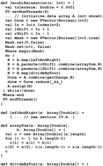
V. SAMPLE PARALLEL PROGRAM:JACOBI RELAXATION After describing the PVector class and its associated methods (operations), we can now present a sample data
parallel Scala program for solving Laplace‘s Equation using
the Jacobi Relaxation algorithm. Consider a two-dimensional (square) conducting metal sheet with the voltage held constant along the four boundaries. The resultant voltage v(x, y) at all the internal points is described
by Laplace‘s Equation in two dimensions:
def JacobiRelaxation(n: Int) = { val tolerance: Double = 0.0001 PV.setNumThreads(4)
... // Initialize data array A (not shown) var Done = new PVector[Boolean](n+2) val In = Init.Index(n+2)
val lShift = In + 1 val rShift = In - 1
val Mask = new PVector[Boolean](n+2,true) Mask.set(0,false)
Mask.set(n+1, false) Where.begin(Mask) do {
B = A.map(leftAndRight)
B = A.permute(rShift).combine(arraySum,B) B = A.permute(lShift).combine(arraySum,B) B = B.map(divideByFour)
Done = A.combine(getChange,B) done = Done.reduce(_&&_) A.assign(B)
} while(!done) Where.end PV.endThreads() }
def leftAndRight(a: Array[Double]) = { ... // see section IV.A }
def arraySum(a: Array[Double], b: Array[Double]) = {
val c = new Array[Double](a.length) for {i <- 1 to b.length-2}
c(i) = a(i) + b(i)
c(0) = a(0); c(c.length-1) = a(a.length-1) c
}
def divideByFour(a: Array[Double]) = { val b = new Array[Double](a.length) for {i <- 1 to b.length-2}
b(i) = a(i)/4.0
b(0) = a(0); b(a.length-1) = a(a.length-1) b
}
def getChange(a: Array[Double], b: Array[Double]) = { var maxchange: Double = 0.0 var change: Double = 0.0 for {i <- 1 to b.length-3} { change = a(i)-b(i)
if (change < 0) change = -change
if (change > maxchange) maxchange = change }
maxchange < tolerance }
0 2 2
2 2
y v x
v
This equation can be solved numerically using a two-dimensional array of discrete points across the surface of the metal sheet. Initially, the points along the boundaries are assigned the appropriate constant voltage. The internal points are all set to 0 intially. Then Jacobi Relaxation is used to iteratively recompute the voltage at each internal point as the average of the four immediate neighboring points (above, below, left, right). Convergence is tested by comparing a desired tolerance value to the maximum change in voltage across the entire grid.
The basic data structure is a two-dimensional (n by n) array of Double values, representing the voltage at each point on the metal sheet. For data parallel execution, a PVector A is created, each of whose elements is a single row from the two-dimensional array. Thus, PVector A has n elements, each one of which is a one-dimensional array:
Array[Double](n). This data parallel PVector provides a
virtual processor for each row of the original two-dimensional array. To recompute the value at each point, the four immediate neighboring points are needed. The left and right neighboring points are easy to find because they are in the same row, and therefore the same element of the PVector A. However, the neighboring points in the rows above and below are in neighboring elements of the PVector A. Access to these is implemented by shifting A left or right using the permute operation described in section IV.C. The data parallel Jacobi Relaxation algorithm in Scala is shown in Fig. 3.
The main body of the algorithm is the do-while loop in the JacobiRelaxation function body. Prior to the loop are the initializations which create the boolean WhereMask and the lShift and rShift PVectors to assist in the left-shift and right-shift permutations, respectively. During the looping, PVec-tor A contains the initial value of the voltage at each point, and the new recomputed values are stored in PVector B. At the end of each iteration, the assign operation copies the values from B back to A, in preparation for the next iteration. In the first operation of the loop, the user-defined operation LeftandRight( ) is used to add the left and right neighboring values to each point. The map operation causes each virtual processor to apply the function LeftandRight( ) to the corresponding element of PVector A. The result is stored temporarily in vector B.
In the following instruction, the permute operation shifts A right and then uses combine to add the corresponding element of B in each virtual processor. This requires an additional user-defined operation arraySum( ), which is then used again to add the left-shift of A to B. Finally, the resultant sum of the neighbors is divided by four using the user-defined function divideByFour( ). This completes the calculation of the new value at each point as the average of the four immediate neighboring points. The user-defined operation getChange( ) determines if the change at each point is less than the desired tolerance. The result is a boolean PVector Done that is aggregated into a single boolean value done by the reduce operation.
Notice the use of the Where.begin(Mask) operation at
the start of the do-while loop. This plays a key role in the correctness of the algorithm. Since the voltage at the boundary edges of the two-dimensional grid are held constant, the relaxation must only be applied to the internal points and not the boundaries. Element 0 of PVector A is the top row of the grid, and element n+1 is the bottom row. Both of these rows must be held constant as the internal points are modified by the relaxation. This is accomplished by setting Mask(0) and Mask(n+1) to false, so that all the PVector operations inside the do-while will not be applied to A(0) and A(n+1).
VI. LIBRARY IMPLEMENTATION
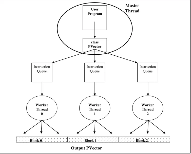
The basic structure of our implementation of PVectors in the library is illustrated in Fig. 4. The User Program is embedded in the Master Thread, along with the PVector class. Each collection-oriented library operation in the User Program will invoke a method in the class PVector. However, the actual computation to implement the operation is performed by the Worker Threads in parallel. Each Worker Thread has an Instruction Queue containing the sequence of operations it is to perform. The PVector class puts the instructions for the Workers into the Instruction Queues. Each Worker will have the same sequence of instructions in its Queue. We do not permit any out-of-order execution by the Workers.
The output data PVector is simply divided among the Worker Threads by using contiguous blocks as illustrated in Fig. 4. If the PVector has length 300, then the first block of 100 is assigned to Worker Thread 0, the next block of 100 to Worker Thread 1, and the last block of 100 to Worker Thread 2. Input PVectors are also partitioned into blocks in the same way. The total number of Worker Threads is determined by the user with the library function call PV.setNumThreads( ). Using this block allocation technique, it is completely predictable in advance which Worker Thread will be operating on each element of the PVector, based only on the length of the PVector and the total number of Workers.
The operator fusion is facilitated by the PVector class in the following way: as soon as the PVector class receives a method invocation from the User Program, it allocates an empty PVector (with no data) to serve as the container for the output data from the Worker Threads, and returns an object reference to this PVector to the User Program. The User Program then continues executing even though the actual data to fill the output PVector has not yet been created by the Worker Threads. This implementation technique does not cause any errors because the User Program cannot directly access the data inside a PVector — it can only access the data indirectly by calling methods in the PVector class.
executing independently without having to synchronize with each other after each PVector operation.
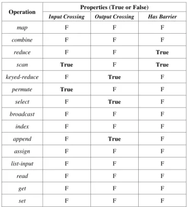
However, depending on the nature and implementation of the specific sequence of requested PVector operations, it is sometimes necessary for some Thread synchronization. Sometimes the Worker Threads must execute a barrier synchronization, and sometimes the Master Thread must participate in this synchronization. Since our library implementation clearly has the isolation and partitioning properties described in section III, we can use the operator fusion algorithm of section IIIC to determine when a barrier (or strong barrier) is needed. The input data for this algorithm is the OpInfoTab shown in Table I with the basic properties of each of the fifteen operations in our collection-oriented library. Only the properties InputCross, OutputCross, and HasBarrier are shown because these are the most interesting and are implementation dependent. The other four properties follow obviously from the definition of each operation. The abundance of False values in this table shows that our implementation has ample opportunity for operator fusion.
To illustrate the principle of operator fusion, consider the following series of data parallel operations starting with data PVectors A, B, C:
T1 = A.map( _*2.0 ) // T1 = 2*A T2 = T1.combine( _+_ , B ) // T2 = T1 + B D = T2.combine( _/_ , C ) // D = T2/C
Assume three Worker Threads perform these operations by dividing the PVectors into blocks as described above. The Worker Threads could perform a synchronization barrier after each operation. However, this is not necessary because the intermediate results computed by the Workers do not cross the block boundaries. Worker 0 reads and writes only elements in block 0 of PVectors A, B, C, D, T1, T2. Similarly, Worker 1 reads and writes only elements in block 1 of all the PVectors. Worker 2 uses only elements in block 2. Therefore, there is no possibility of interference between the Workers: they read and write separate elements of the PVectors. Thus, the (map, combine, combine) sequence of data parallel operations could be fused within each Worker Thread without any intervening barriers. This operator fusion of data parallel operations greatly improves the performance.
User Program
class PVector
Instruction Queue
Instruction Queue
Instruction Queue
Worker Thread
0
Block 0 Block 1 Block 2
Worker Thread
1
Worker Thread
2
Output PVector
Master
Thread
TABLE I. PROPERTIES OF DATA PARALLEL OPERATIONS
Operation Properties (True or False)
Input Crossing Output Crossing Has Barrier
map F F F
combine F F F
reduce F F True
scan True F True
keyed-reduce F True F
permute True F F
select F True F
broadcast F F F
index F F F
append F True F
assign F F F
list-input F F F
read F F F
get F F F
set F F F
A. Instruction Queue
As illustrated in Figure 4, each Worker has its own instruction queue to receive the sequence of required operations from the class PVector. Each data parallel operation in the User Program requires invocation of a method in the class PVector, which in turn will encode the requested data parallel operation into an instruction, and write this instruction into the queue of each Worker thread. When there is a series of data parallel operations generated from the User program, the instructions will build up in the Worker instruction queues.
Our implementation uses a very simple form for the instructions with a numeric opcode field and five additional fields for arguments:
Instruction Field Type 1 Int 2 PVector 3 PVector 4 PVector
5 function of one parameter 6 function of two parameters
Each of the fifteen data parallel operations currently included in the library has a specific numeric opcode ranging from 1 to 15, which is placed in Instruction Field 1. To produce an output, the data parallel operations do not modify the input PVector, but rather create a new PVector and return it to the caller. The initial allocation of the output PVector is done in the class PVector. Then a reference to the empty output PVector is passed in Field 2 to the Workers, which write the data into it. Field 3 is used for a reference to the input PVector. Some data parallel operations, such as keyed-reduce, also require a reference to a third PVector, which is placed in Field 4. Fields 5 and 6 are used for
references to user-defined functions supplied as parameters to many of the data parallel operations, such as reduce and combine.
These simple instructions represent a kind of data parallel machine language with fifteen opcodes. Each instruction is conveniently represented in Scala as a tuple. The instruction queue of each Worker Thread is implemented by the library class LinkedBlockingQueue() as found in the library java.util.concurrent. The writing of the queue from the Master Thread and the reading of the queue from the Worker Thread is done in parallel. Therefore, proper synchronization is needed to make the queue work properly. This is all handled within the library code of
LinkedBlockingQueue().
With this implementation, each Worker Thread is free to execute its instructions at its own speed, working on its assigned block of the PVector. Thus, the required vertical integration of the data parallel operations results naturally from this implementation. However, some of the operations in our library may cause Worker Threads to cross block boundaries into portions of the PVector assigned to other Workers. For these operations, a barrier synchronization among the Workers may be required either before or after the operation.
B. Barrier Synchronization
As briefly explained in previous sections, the ability to do operator fusion of the data parallel PVector operations originates from the fact that all the Worker Threads are assigned to disjoint blocks of the PVectors. As long as the reading and writing of data values by each Worker remains within its own block, there is no possibility of any timing-dependent errors, and the Workers can just proceed independently at their own relative speeds. However, among the fifteen operations in our data parallel library, there are some operations that do require the Workers to cross block boundaries and either read or write an element in a block assigned to another Worker.
Consider a simple example of the following sequence of data parallel operations in a User program:
T1 = A.map( _*2.0 ) // T1 = 2*A T2 = T1.permute(Index) // permute T1
The first operation creates a new PVector T1 by multiplying every element of PVector A by 2.0. Then the second operation permutes (reorders) the elements of T1 to create a new PVector T2. This is illustrated in Fig. 5. Assume there are three Worker Threads and the PVector size is 300. As shown in the Figure, each Worker is assigned a distinct block of 100 elements from PVector A and T1. Therefore, the multiplication by 2.0 can proceed independently in each Worker.
value 216.6 must be written into T1 by Worker 1 during the previous data parallel operation (multiply A by 2.0).
If Worker 0 is faster than Worker 1, it may try to retrieve element 150 from T1 before Worker 1 writes, causing the old value to retrieved. To prevent this type of data race error, the first operation (multiply A by 2.0) must be completed before the permute operation begins. Thus, a barrier synchronization of all the Worker Threads is required between the operations, as shown in Fig. 5.
Using the general terminology developed in section III, the value 216.6 is an example of a cross-thread data element. For convenience, the definition is repeated here: a data element e of a DP-Collection v is said to be a cross -thread data element if there exist DP-Operations di and dj,
such that eϵ O(dj, v, k) and eϵ I(di, v, m) and km. In this
example, operation dj is the map operation in the assignment
to T1 and operation di is the permute operation in the
assignment to T2. The PVector v is T1, and the value 216.6 is data element e. Thus, we have eϵ O(map, T1, 1) and eϵ I(permute, T1, 0). Since 1 0, e satisfies the definition of a cross-thread data element, and therefore, a barrier synchronization is required after the map operation. This requirement for a barrier will be detected by the Operator FusionAlgorithm of Fig. 2, which is included as part of our data parallel library implementation.
In our block-based implementation, any data parallel operation that may cause a Worker to cross block boundaries will create a cross-thread data element and therefore requires some kind of barrier synchronization of the Workers. If the boundary crossing occurs in one of the input PVectors to an operation, then a barrier is required before the operation begins, as is the case with the permute operation illustrated in Fig. 5. Using the general terminology developed in section III, the permute operation has an inputcrossing, as shown in Table I. If the boundary crossing occurs in the output PVector of an operation, it is called an output crossing, and a barrier is required at the end of the operation. In Table I, we see a few input and output crossings for our data parallel library operations. However, the vast majority of operations do not have crossings, resulting in ample opportunity for operator fusion.
C. Master Thread Synchronization
One additional consideration is synchronization between the Master and Worker Threads. The Master Thread contains the User program and class PVector (see Fig. 4). When an operation is requested by the User program, the class PVector sends an instruction to each Worker Thread, then returns to the User program before the operation is actually completed by the Workers. The User program continues to execute and may request additional data parallel operations. Thus, the User program can progress far ahead Worker
Thread 0
216.6 Worker
Thread 1
Worker Thread
2
Block 0 Block 1 Block 2
150
216.6 A
T1
Index
T2
Barrier required here