COMPUTING MAX FLOWS THROUGH CUT NODES

doi: 10.1590/0101-7438.2017.037.03.0437

COMPUTING MAX FLOWS THROUGH CUT NODES

Jo˜ao Paulo de Freitas Araujo

, Fernanda Maria Pereira Raupp

,

Jos´e Eugenio Leal

and Madiagne Diallo

Received November 15, 2016 / Accepted October 23, 2017

ABSTRACT.In this work, the presence of cut nodes in a network is exploited to propose a competitive method for the multi-terminal maximum flow problem. The main idea of the method is based on the relation between cut-trees and cut nodes, which is observed in the context of sensitivity analysis on the variation of edges capacities. Computational experiments were conducted with the proposed algorithm, whose re-sults were compared with the ones of Gusfield, for randomly generated and well-known instances of the literature. The numerical results demonstrate the potential of the method for some classes of instances. Moreover, the proposed method was adapted for the single maximum flow problem, but failed to improve existing running times for the very same classes of instances.

Keywords: maximum flow, cut-tree, cut nodes.

1 INTRODUCTION

Computing the maximum flow value between a source and a terminal node of a given network is a classical problem in the context of network flows. Its extension, namely themulti-terminal maximum flow problem, consists of finding the maximum flow values between all pairs of nodes of an undirected network. These problems have several applications, especially in the field of logistics, biology, telecommunications and energy, see for example, Cohen & Duarte Jr. (2001), Tuncbag et al. (2010) and Diallo (2011).

It is noteworthy that the multi-terminal maximum flow problem differs from the multi-com-modity flow problem. While, in the latter problem, mixed flows between multiple pairs of origins and destinations share the network, in the former, although we compute the maximum flow values for all pairs of the network nodes, there is a single flow between a source node and a destination node in the network at a time.

*Corresponding author.

1Departamento de Engenharia Industrial, PUC-Rio, Rua Marquˆes de S˜ao Vicente, 225, G´avea, 22451-900Rio de Janeiro, RJ, Brasil. E-mails: [email protected]; [email protected]; [email protected]

Ford & Fulkerson (1973) popularized the maximum flow problem in the ’50s. Through the demonstration of the connection between a maximum flow value and a minimum cut capac-ity, they sophisticatedly solved it. Since then, many improved algorithms have been published to compute the maximum flow values or the minimum cut capacities, including the preflow-push algorithm from Goldberg & Tarjan (1986), which we will use in this work.

Regarding the multi-terminal maximum flow problem of a given undirected networkGwithn nodes, one can solve it naively, by runningn(n−1)/2 times a maximum flow algorithm between all unordered pairs of nodes ofG. However, Gomory & Hu (1961) developed a method to com-pute the maximum flow values ofG, by just running(n−1)times a maximum flow algorithm. Its output, called cut-tree, summarizes the maximum flow values and identifies a minimum cut between any pair of nodes. After that, Gusfield (1990) presented a simpler procedure to obtain the same cut-tree, but also using(n−1)times the maximum flow algorithm. Then, Goldberg & Tsioutsiouliklis (2001) conducted a study comparing computationally three variations of the Gomory and Hu algorithm and the Gusfield algorithm. For the unweighted case, when each edge has one-unit capacity, Bhalgat et al. (2007) showed a faster algorithm that does not use a maxi-mum flow algorithm as internal procedure.

Elmaghraby (1964) introduced the sensitivity analysis on multi-terminal flows, studying the ef-fects on the maximum flow of a network through the variation of a single (parametric) edge capacity. Later, Barth et al. (2006) extended that study to the case of more than one paramet-ric edge, noting that a total of 2k cut-trees is sufficient to compute all maximum flows for any parameter value, beingkthe number of parametric edges in the network.

In this work, given an undirected network G, by using the theory of sensitivity analysis on multi-terminal network flows under edge capacity variations, we introduce a theoretical property that relates cut nodes and cut-trees. Based on such a property, we propose a new approach for the computation of cut-trees for networks that contain cut nodes. Similarly, a single maximum flow can be computed in parts, if there are cut nodes in the path between the source and the terminal node.

Computational experiments are conducted to compare the running times of the proposed proce-dures with respect to the traditional ones. For these experiments, four instances families are used: PATH and TREE, from Goldberg & Tsioutsiouliklis (2001), CACTUS, from Husimi (1950), and PARTED that we specially developed for the experiments. When a given undirected network contains cut nodes, the numerical results show that the computation of cut-trees with the pro-posed method is effective. However, for the same test instances it seems not the case, when we apply an adaptation of the method to solve particularly the single maximum flow problem.

2 NOTATION AND BASIC CONCEPTS

From now on, we assume that the reader has basic knowledge of graph and network flows theories and problems. Reference books include Ford & Fulkerson (1973), and Hu & Shing (2002).

LetG=(V,E)be a connected undirected graph, consisting of a setV ofnnodesv, and a setE ofmedgese, where each edge is an unordered pair[i,j]of nodes inV. Anetworkis a graphG associated with acapacityfunction over the edgesc: E → R+. Aflowfrom a source nodesto

a terminal nodetinGis a function f : E→ R+with the conservation property at each nodev,

except forsandt

i∈V

f(i, v)=

j∈V

f(v, j) ∀v∈V\{s,t},

and the capacity constraint

∀i,j ∈V, f(i,j)≤c(i,j).

Observe that edges can be represented by two arcs of opposite directions. Therefore, unlike an arc, an edge has no direction, that is, it has two opposite directions at once. Thus, an undirected network has the same structure as a directed symmetric network, where each arc has the same capacity of the original edge, allowing equal capacity to either direction. It is important to note that, when a flow passes through a capacitated edge, it uses only one arc, never both. Hereafter, we will deal only with undirected networks.

We denote by(s - t)the cut separating the nodess andt, byc(s -t)the capacity of the cut (cut value), and by(X,X)a cut separating the nodes of a graph into two complementary subsets X andX. Among all possible cuts separatingsandt, one with the smallest capacity is called aminimum cut, and its capacity is the maximum flow value betweens and t, which will be represented by fs,t.

After observing the existence of at mostn−1 distinct values of maximum flow in an undirected network withn nodes, Gomory & Hu (1961) developed a method that obtains then(n −1)/2 values of maximum flows using a node contraction scheme and running onlyn−1 times the maximum flow algorithm. The result is expressed by a cut-tree defined as follows.

Definition 2.1. Acut-treeof a network G =(V,E)is a tree CT =(V,E′)obtained from G, with weighted edges and the same set of nodes V . A cut-tree CT has the following properties:

1. Equivalent flow tree: the value of the maximum flow between any s and t of G is equal to the value of the maximum flow in CT between s and t , that is, the smallest edge capacity on the unique path connecting s to t in CT . Thus, the maximum flows between all pairs of nodes in G are represented in CT ;

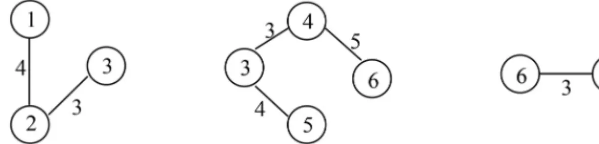
Figure 1 illustrates an example of a cut-treeCT constructed from a networkG. As we can see, by the properties mentioned above, the minimum cut between nodes 2 and 3, and nodes 1 and 2, are respectively reflected by the edges[2,3]and[1,2]of the cut-treeCT. Its maximum flow values are the capacities of these edges, in this case 3 and 4, respectively. The minimum cut between nodes 1 and 3 is reflected, in turn, by the edge[2,3]inCT, with maximum flow value equal to 3.

Figure 1– Example of a cut-treeCTof a networkG.

In general, there are several cut-trees for the same network. The cut-tree will be unique only if all the(s-t)minimum cuts of the network are unique.

Gusfield (1990) presented a very simple procedure that builds a cut-tree without using contrac-tion of nodes. Its implementacontrac-tion is very easy: it takes only five addicontrac-tional lines of code to any algorithm that computes a minimum cut. Like the method of Gomory and Hu, Gusfield’s method solves the multi-terminal maximum flow problem with(n−1)executions of a maximum flow algorithm.

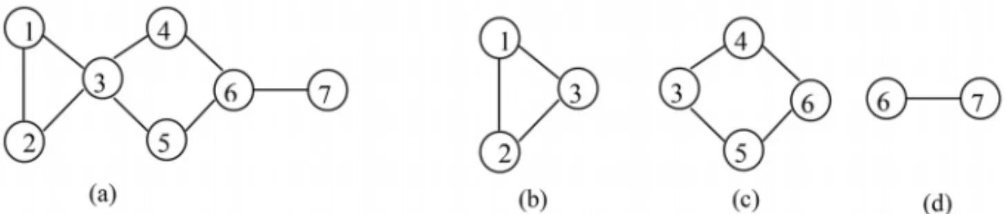
Definition 2.2. A node i of a connected graph G is called acut nodewhen G\{i} is not con-nected.

As for illustration, nodes 3 and 6 are cut nodes of the graph showed in Figure 2(a), as we can verify respectively in Figures 2(b) and 2(c).

Figure 2– Illustration of cut nodes.

Definition 2.3. Abiconnected componentof a graph G is a maximal connected subgraph B of G containing no cut nodes, where the term “maximal” refers to the state that any inclusion of a node in B creates a cut node in B.

Figure 3– The graph (a) and its three biconnected components (b), (c) and (d).

3 PROPERTIES OF CUT NODES

In this section, we introduce some theoretical results that allow an innovative computation of both the single and the multi-terminal maximum flow problems, by exploiting the presence of cut nodes in networks. For the case of the multi-terminal maximum flow problem, the property comes up from its parametric version, formulated in the light of the theory of sensitivity analy-sis on multi-terminal maximum flows. In general terms, this theory studies the behavior of the maximum flows values between the all pairs of nodes in a network under variations of edge capacities.

Barth et al. (2006) examined the parametric problem considering the increasing variation of the capacity of a single edge. The problem can be formulated as follows for a pair of nodes.

LetG = (V,E)be a network with source nodes and terminal nodet. Consider an edgee= [i,j] ∈ E with non-negative capacityc(e) = λ. The goal is to determine the maximum flow value betweensandtwith the increasing variation ofλ.

The cited authors observed that, for a network that has only one edge with parametric capacity, the variation of this capacity may not influence the values of maximum flows (and minimum cuts) for various pairs of nodes. Denoting by f_s,tλ the maximum flow value betweensandtwhen the capacity of the edgeeisλ, they stated the following result.

Lemma 1 (Barth et al. (2006)).Let G =(V,E)be a network with n nodes, and e= [i,j] ∈ E such that c(e)=λ. Let s and t be a pair of nodes of G and CTα_{a cut-tree when c(e)=α. If}

the path connecting s to t Ps,t in CTαhas no edge in common with Pi,j, then fs,tλ = fs,tα, ∀λ >

α≥0.

Proof. Using the cut property of the cut-trees (Definition 2.1, item 2), one can show that there exists a minimum cutCα

s,t separatingsandtwhere both nodesiandj(e= [i,j])are in the same

side of the minimum cut. Therefore, the cut does not containeforλ > α, and it is insensible to

the variation ofλ.

Still, for the next result of Barth et al. (2006), the following definition is necessary.

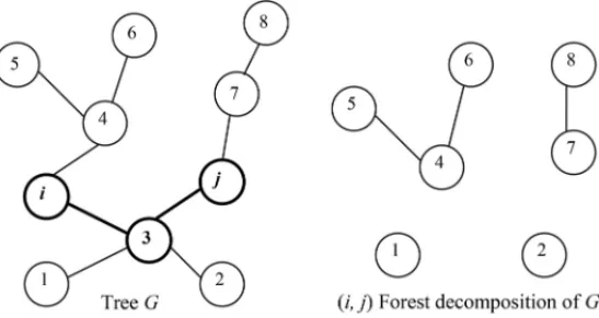
Definition 3.1.Let G =(V,E)be a connected and acyclic network, i.e., a tree. Let i and j be a pair of nodes of G and Pi,j the (unique) path connecting them. The(i,j)forest decomposition

For example, consider the treeGand the pathi-3-j inGon the left of Figure 4. Then, the(i,j) forest decomposition ofGis formed by the four subtrees on the right of Figure 4.

Figure 4– Example of a(i,j)forest decomposition of a given treeG.

Lemma 2 (Barth et al. (2006)). Let G be a network with an edge e = [i,j]with parametric capacity. Let CTα be the cut-tree when c(e)=α. Let Fi,j be the(i,j)forest decomposition of

CTα. For each tree T ∈ Fi,j, there exists a cut-tree of G with c(e)=λ > αthat contains T as

subtree.

Proof. To see this proof, please, refer to the work of Barth et al. (2006). Now, we introduce the following results.

Lemma 3.If two nodes belong to a biconnected component A, the maximum flow between them can be computed considering A as a graph itself.

Proof. Ifsandtare nodes ofGinA, there is no path betweensandtthat contains a node not

inA.

Before we introduce the next result, it is important to observe that:

• The affirmation that a given edge is not contained in a network is equivalent to say that this edge is contained in the network with null capacity. Therefore, adding an edge to a network can be understood as varying positively its capacity from zero.

Lemma 4.The cut-tree of a graph is the union of the cut-trees of its biconnected components.

Proof. LetG be a graph with a unique biconnected component A, which is the graph itself. LetCT andCTA be the cut-trees ofGandA, respectively. By adding edge after edge, and the

and j inCT. Since, at every step, Pi,j doesn’t have edge in common withCTA, according to

Lemmas 1 and 2, the cuts inCTA are not influenced by the process and they can be part of the

finalCT. To conclude the proof, from Lemma 3, the nodes ofAreside on the same side aszin all minimum cuts between nodes fromB, which leads to the result thatCTA can be a subtree of

the finalCT.

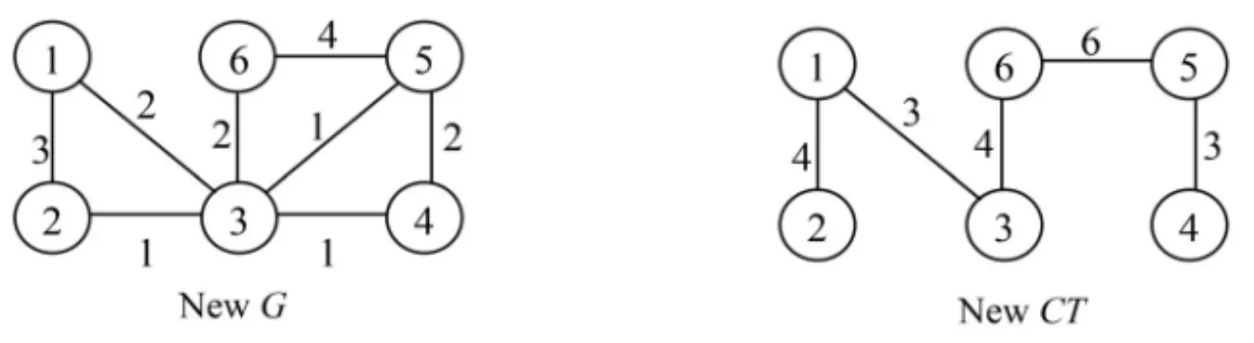
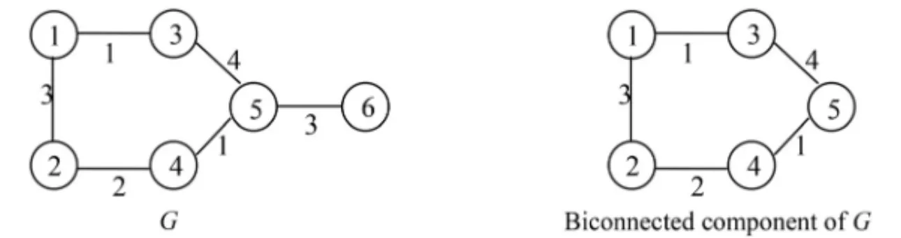
Next we show an example of the proof of Lemma 4. Consider the networkGand its cut-treeCT showed in Figure 5.

Figure 5– NetworkG(left) and its cut-treeCT (right).

Based on Lemma 1, if we add to the networkGedges[3,6],[3,5],[3,4],[4,5]and[5,6], one by one, these additions would not influence the cuts inCT represented by the edges[1,2]and

[1,3]. Furthermore, the newCT, according to Lemma 2, could contain these cuts. At last, from Lemma 3, node 3 will be adjacent to node 1 in the newCT. Figure 6 illustrates the new network and its correspondingCT.

Figure 6– Network NewG(left) and its cut-tree NewCT(right).

For the case of determining the single maximum flow between a source and a terminal node, we state that:

Lemma 5.Let s and t be a pair of nodes of a network G. If a path P between s and t traverses x cut nodes of G, then the maximum flow between s and t is the minimum value among the maximum flows between(s,z1), (z1,z2), . . . , (zx,t), where z1,z2, . . . ,zxare the cut nodes of G

in P in the order they are traversed from s to t .

Proof. The proof is simple. If there are cut nodes ofGin P, the removal ofz1disconnects s from t, and so all the flow that leavess must pass throughz1. The same result is true for

4 PROPOSED METHODS

Based on Lemma 4, if a network has cut nodes, one can solve the multi-terminal maximum flow problem by computing the cut-trees of each of its biconnected components and joining them at the end. Next, we describe the outline of the proposed method, namely CN.

For computing the maximum flow between all pairs of nodes in an undirected network G = (V,E)withnnodes and capacities on the edges, CN identifies the biconnected components and performs a test. If no biconnected component has more than 80% ofn nodes, then the method applies the Gusfield algorithm on each biconnected component. Finally, the cut-tree of G is achieved by joining all the cut-trees of the biconnected components. Otherwise, if there is a biconnected component with more than 80% ofnnodes, it applies Gusfield algorithm toG.

Observe that the if-then condition is different from just having a cut node. It avoids the situation shown in Figure 7, where a biconnected component has almost the size of the network. In this situation, it becomes difficult to compensate the overhead of managing biconnected components with computations of maximum flow in networks considerably smaller than the original. The choice for the percentage of 80% will be discussed in Section 5. Regarding the if-else condition, note that a network without cut nodes has only one biconnected component, that is, the network itself. Figure 8 shows the pseudo-code of the method CN.

Figure 7– NetworkG (left) and its biconnected component with more than 80% of the nodes (right).

Input:G

1 Identify all biconnected components inG;

2 ifno biconnected component has more than 0.8n nodesthen

3 | Apply Gusfield algorithm to each biconnected component separately;

4 | Join all the cut-trees of the biconnected components into a unique cut-treeCT; 5 else

6 | Apply Gusfield algorithm toGto getCT; 7 returnCT;

Figure 8– Pseudo-code of CN.

Given the network instance showed in Figure 9, in the following we illustrate the application of CN.

Figure 9– NetworkG.

First, the algorithm finds nodes 3 and 6 as cut nodes. Then, it identifies three biconnected com-ponents inG(line 1), which are shown in Figure 10.

Figure 10– Biconnected components ofG.

As no biconnected component ofGhas more than five nodes (line 2), the algorithm computes, through Gusfield algorithm, the cut-tree of each biconnected component (line 3). The resulting cut-trees are illustrated in Figure 11.

Figure 11– Cut-trees of the biconnected components ofG.

Finally, all the cut-trees of the biconnected components are joined to form the cut-tree ofG (line 4), as in Figure 12.

Regarding the single maximum flow problem, we can implement a new approach based on Lem-mas 3 and 5. After identifying the biconnected components of the network and a path between the source and the terminal nodes, the method computes, under the condition that there is no biconnected component with more than 0.8n nodes, all (s,z1), (z1,z2), . . . , (zx,t)maximum

flows values. Finally, it returns the minimum value among them. Otherwise, if there is a bicon-nected component with more than 0.8nnodes, a maximum flow algorithm is applied toG. Note that, ifsandtare in a same biconnected component, there will be noznodes, and the method will run just once the single maximum flow algorithm. The choice for the size of 0.8n, in the condition of the algorithm, will be also discussed in Section 5. Figure 13 shows the pseudo-code of this method, namely MaxFlow CN.

Input:G,s,t

1 Identify all biconnected components inGand a path Pbetweensandt; 2 ifno biconnected component has more than 0.8n nodesthen

3 | Letzbe the current node while traversingPfromstot; 4 | Setzas the node adjacent tos;

5 | whilez=tdo

6 | | ifzis a cut node ofGthen

7 | | | Compute fs,z in the biconnected component that contains bothsandz;

8 | | | s←z;

9 | | z←next node inP;

10 | Compute fs,z in the biconnected component that contains bothsandz;

11 | maxflow←minimum value among all fs,z;

12 else

13 | maxflow←Compute fs,t inG;

14 returnmaxflow;

Figure 13– Pseudo-code of MaxFlow CN.

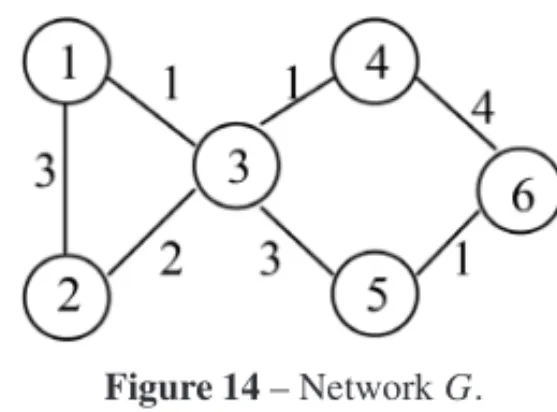
Let us exemplify the application of MaxFlow CN algorithm in the network shown in Figure 14, takings=1 andt=6.

Figure 14– NetworkG.

Figure 15– Biconnected componentsAandBofG.

As no biconnected component ofGhas more than four nodes (line 2), the algorithm sets zas node 2 (lines 3 and 4). Then, since 2=t, the commandwhileis executed (line 5). As node 2 is not a cut node (line 6),zis now updated as node 3 (line 9), andwhileis executed again, since 3 = t. Now, aszis a cut node (theifcondition is true), f1,3 is computed in the biconnected component Aandsis updated to node 3 (lines 6, 7 and 8). In this case, f1,3=3 with minimum cut composed by edges[1,3]and[2,3]. In the third iteration of the loopwhile, withzset as node 5, theif condition is not true. Then, z is updated to node 6 = t, causing the stopping ofwhile. A maximum flow algorithm is run in B, resulting in f3,6 = 2, with minimum cut composed by[3,4]and[5,6](line 10). Finally, the maximum flow value between nodes 1 and 6 is the minimum value between f1,3and f3,6(line 11), which is 2.

Since the method seeks the minimum fs,z value, we compute each fs,z faster by limiting it to

an upper bound variableu. Initiallyu =M, where M is a big number, and when fs,z <u, then

u = fs,z. The maximum flow algorithm will perform lesser operations as no flow can exceed

u. In the example above, the variableu is updated twice, from M to 3 and from 3 to 2, after computing respectively f1,3and f3,6.

As in CN, the algorithms of Hopcroft & Tarjan (1973) and the highest-label preflow-push of Goldberg & Tarjan (1986) were used in MaxFlow CN to identify the biconnected components and to compute the maximum flows, respectively.

5 COMPUTATIONAL EXPERIMENTS

In this section, we report computational experiments with CN and MaxFlow CN, proposed here, in comparison with the algorithms of Gusfield (GUS) and Goldberg and Tarjan (MaxFlow), which were implemented by Skorobohatyj (2011). Moreover, we show some numerical tests that empirically defined the condition in line 2 in CN and MaxFlow CN. In the four algorithms, the maximum flow value is computed with an optimized version of the highest-label preflow-push algorithm, where the resulting flow is not computed for all edges.

For the experiments, the instances were created by the generators PATHGEN and TREEGEN, from Goldberg & Tsioutsiouliklis (2001), and PARTEDGEN, CACTUSGEN, and TESTGEN, specially developed here for this purpose. The desired characteristics of the test instances are: the presence of cut nodes or the high chance of having cut nodes in the generated graphs.

Let us denote the parameters used by the five generators:nthe number of nodes in the graph,d the density of the graph given in terms of a percentage of arcs (that indirectly defines the number of arcsm),Pthe edge capacity factor, andSthe seed of the generator. As follows, we introduce them briefly.

Given the path length (parameter k), the PATHGEN builds a path of k−1 edges and con-nects the remainingn−knodes to the path nodes at random. Then, it adds edges at random to achieve the desired number of arcs and to make the minimum cut problems more difficult. For the PATHGEN, thekvalue determines the path shape. For example, ifk=n, then we get one path through all the nodes; ifk=1, then we have all nodes sharing an edge with node 1.

Given the tree shape (parameterk), the TREEGEN generator builds a tree by connecting node i,i =2, . . . ,n, to a randomly chosen node in{1,min{i−1,k}}. Then, it adds edges at random to achieve the desired number of arcs and to make the minimum cut problems more difficult. The value ofkdetermines the shape of the tree. For example, ifk=1, then the tree is a star. If k=n−1, then the tree is obtained by connecting each node, except the first one, to a randomly chosen preceding node.

Given the number of biconnected components (parameter k), the PARTEDGEN builds a graph withk−1 cut nodes linking biconnected components of equal size. After building a path through all the nodes in the first step, it adds strategic edges to create k-edge disjoint cycles of size approximatelyn/k. Finally, it adds edges at random in each biconnected component to achieve the desired number of arcs.

To explain CACTUSGEN, the following definition is necessary.

Definition 5.1.A connected graph in which every two cycles have at most one node in common is acactus graph.

Given the number of cycles (parameter k), the CACTUSGEN generator builds a cactus graph withk cycles. We created two types of the generator: CACTUS PATHGEN and CACTUS -STARGEN. In the first type, a path through all the nodes is built and thenkedges are added to formk-edge disjoint cycles, and, in the second one, allkcycles have the same size and one node in common. In both, the density parameterdis not considered, since in these caseskdefines the number of edgesm.

In the computational experiments, we consider up to three distinct seeds(S = 1,2,3), except for the generation of PARTED instances. The edge capacities are chosen uniformly at random from the interval[1, . . . ,100P]. We set the factor P =1 when generating all the instances, as well asn=1000. We observe that this value ofnis relative large in relation to the ones used in Goldberg & Tsioutsiouliklis (2001). The inputs of algorithms MaxFlow and MaxFlow CN were s =1 andt =1000, so thatsandt were in different biconnected components in the generated instances.

To estimate the maximum size of a biconnected component, needed for the condition in line 2 of the algorithms CN and MaxFlow CN, numerical tests were performed for instances of the family TEST, with the following variants of CN and MaxFlow CN:

• CN 0 and MaxFlow CN 0: CN and MaxFlow CN implemented with the size 0.0*n in line 2 condition, i.e., for these variants, the condition is never satisfied;

• CN 1 and MaxFlow CN 1: CN and MaxFlow CN implemented with the size 1.0*n in line 2 condition, i.e., for these variants, the condition is always satisfied.

Hereafter, for each class of the test instances we show the comparison of the running times ob-tained by the proposed algorithms. The running times obob-tained by CN 0, CN 1, MaxFlow CN 0 and MaxFlow CN 1 are reported in Table 1. The running times obtained by the algorithms CN, GUS, MaxFlow CN and MaxFlow for the PARTED and PATH generated instances are summa-rized in Tables 2 and 3, respectively. The results obtained for the TREE generated instances are shown in Table 4. Tables 5 and 6 show the running times for the CACTUS PATH and CAC-TUS STAR instances, respectively. For each test instance, the running time refers to the median of five runs of the algorithm given in microseconds (µs). The symbol∗that may appear next the seed value means that a biconnected component of the graph instance has more than 80% of the nodes of the graph instance.

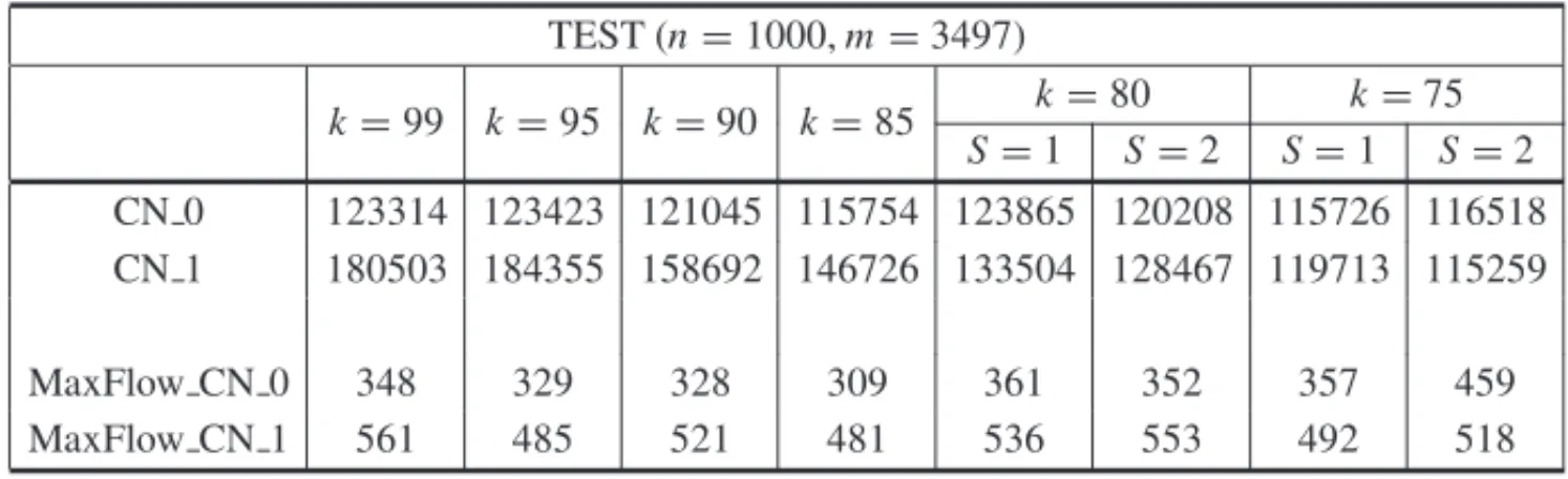
Table 1 – Running time for the TEST instances with n = 1000, m = 3497, k = 99,95,90,85,80,75 andS=1,2.

TEST (n=1000,m=3497)

k=99 k=95 k=90 k=85 k=80 k=75

S=1 S=2 S=1 S=2

CN 0 123314 123423 121045 115754 123865 120208 115726 116518 CN 1 180503 184355 158692 146726 133504 128467 119713 115259

MaxFlow CN 0 348 329 328 309 361 352 357 459

MaxFlow CN 1 561 485 521 481 536 553 492 518

Analyzing the numerical results, we point out that:

Table 2– Running time for the PARTED instances with n=1000,m=3497 andk=2,4,8,16.

PARTED (n=1000,m=3497)

k=2 k=4 k=8 k=16

CN 71204 29685 15059 8394

GUS 97514 95450 94860 94339

MaxFlow CN 433 401 390 424

MaxFlow 260 179 353 121

Table 3– Running time for the PATH instances withn=1000,m=1399,k=250,500,750 andS=1,2,3.

PATH (n=1000,m=1399)

k=250 k=500 k=750

S=1 S=2 S=3 S=1 S=2 S=3 S=1∗ S=2∗ S=3∗

CN 38200 35789 35667 49642 49253 50138 60114 61432 59639 GUS 55046 54261 55628 58469 58095 58162 57825 58748 57192

MaxFlow CN 184 185 191 208 203 194 164 157 156

MaxFlow 180 65 64 71 65 58 76 68 68

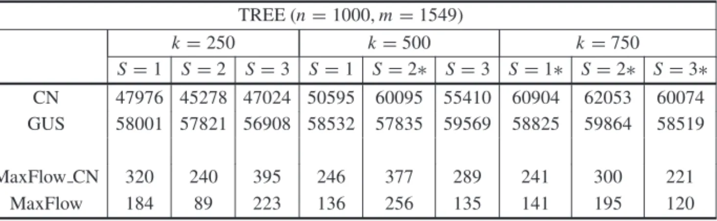
Table 4– Running time for the TREE instances withn=1000,m=1549,k=250,500,750 andS=1,2,3.

TREE (n=1000,m=1549)

k=250 k=500 k=750

S=1 S=2 S=3 S=1 S=2∗ S=3 S=1∗ S=2∗ S=3∗

CN 47976 45278 47024 50595 60095 55410 60904 62053 60074 GUS 58001 57821 56908 58532 57835 59569 58825 59864 58519

MaxFlow CN 320 240 395 246 377 289 241 300 221

MaxFlow 184 89 223 136 256 135 141 195 120

2. Still, for the TEST instances, since MaxFlow CN 1 running time does not get better when the parameterkdecreases, the condition in line 2 of MaxFlow CN was also set to the 80% percentage;

3. For the PARTED instances, when the parameterkincreases, CN performance gets much better than GUS performance;

Table 5– Running time for the CACTUS PATH instances withn=1000, k=10,20 andS=1,2,3.

CACTUS PATH (n=1000)

k=10(m=1009) k=20(m=1019)

S = 1 S = 2 S = 3 S = 1 S = 2 S = 3

CN 8901 9047 8905 4812 4867 4777

GUS 68897 67814 70287 59783 57929 61114

MaxFlow CN 116 117 131 114 130 128

MaxFlow 115 161 121 122 80 52

Table 6– Running time for the CACTUS STAR instances withn=1000, k=10,20 andS=1,2,3.

CACTUS STAR (n=1000)

k=10(m=1009) k=20(m=1019)

S = 1 S = 2 S = 3 S = 1 S = 2 S = 3

CN 9079 9090 9261 5313 5246 5320

GUS 69456 65624 65816 57762 55744 56923

MaxFlow CN 63 65 61 52 51 52

MaxFlow 113 77 70 80 69 34

5. CN running times for PATH instances were up to 35%(k=250,S=3)lower than GUS. For the TREE instances, CN running times were up to 21%(k=250,S =2)lower than GUS;

6. For the generated instances with a biconnected component with more than 0.8n, CN per-forms very close to GUS algorithm, while MaxFlow CN perper-forms worse than MaxFlow;

7. For CACTUS PATH and CACTUS STAR instances, CN outperforms GUS, even better whenkincreases;

8. For almost all instances, MaxFlow obtains better running times than MaxFlow CN.

One possible reason to explain why the performance of CN improves when the parameter k increases in PARTED, CACTUS PATH and CACTUS STAR instances is that the biconnected components of the graphs become smaller. For the PATH and TREE instances, the opposite may occur, that is, whenkincreases, the biconnected components become larger.

Regarding CN’s good performance, we observe that it executesn−1 maximum flow algorithms in subgraphs of the original graph, whereas GUS appliesn−1 maximum flow algorithms in the original graph.

6 CONCLUSION

This work studied the relation between the maximum flows and cut nodes and proposed new approaches to solve the single and the multi-terminal maximum flow problem in graphs with cut nodes, aiming to reduce the running time, i.e., the computational complexity, when compared to the results obtained by classical algorithms.

The computational experiments conducted with the proposed methods used instances gener-ated by PATHGEN, TREEGEN, PARTEDGEN and CACTUSGEN, where the last two were especially developed here. The numerical results pointed out that CN algorithm has better per-formance in comparison to Gusfield algorithm, whereas the MaxFlow CN algorithm could not overcome the MaxFlow algorithm.

Variants of the proposed methods can still be developed and tested. For instance, a comparison study can be done with CN being implemented with Gomory and Hu’s method as subroutine instead of Gusfield’s. Since the maximum flow algorithm implemented by Skorobohatyj, that we used in both MaxFlow and MaxFlow CN, is an optimized version of the Goldberg & Tar-jan (1986) algorithm, tests with the full version are recommended.

REFERENCES

[1] BARTHD, BERTHOME´P, DIALLOM & FERREIRAA. 2006. Revisiting parametric multi-terminal problems: Maximum flows, minimum cuts and cut-tree computations.Discrete Optimization,3(3): 195–205.

[2] BHALGATA, HARIHARANR, KAVITHAT & PANIGRAHID. 2007. AnO(mn)˜ Gomory-Hu Tree Construction Algorithm for Unweighted Graphs. STOC’07 Proceedings of the thirty-ninth annual ACM symposium on Theory of computing, 605–614, June.

[3] COHEN J & DUARTE JR EP. 2001. Fault-Tolerant Routing of Network Management Messages in the Internet. The 2nd IEEE Latin American Network Operations and Management Symposium (LANOMS’2001), 87-98, Belo Horizonte, MG.

[4] DIALLOM. 2011. M´ethodes d’Optimisation Appliqu´ees aux R´eseaux de Flots et T´el´ecoms. Editions universitaires europeennes.

[5] ELMAGHRABYSE. 1964. Sensitivity analysis of multi-terminal flow networks.Operations Research, 12(5): 680–688.

[6] FORDLR & FULKERSONDR. 1973. Flows in Networks. Princeton University Press, Princeton, NJ.

[7] GOLDBERGAV & TARJANRE. 1986. A new approach to the maximum flow problem.ACM Sym-posium On Theory of Computing, 136–146, Berkeley, California, May.

[9] GOMORYRE & HUTC. 1961. Multi-terminal network flows.SIAM Journal of Computing,9(4): 551–570, December.

[10] GUSFIELDD. 1990. Very simple methods for all pairs network flow analysis.SIAM Journal of Com-puting,19(1): 143–155.

[11] HOPCROFTJ & TARJANR. 1973. Efficient algorithms for graph manipulation.Communications of the ACM,16(6): 372–378.

[12] HUTC & SHINGMT. 2002. Combinatorial Algorithms, Enlarged 2nd Ed. Dover Publications, INC, Mineola, New York.

[13] HUSIMIK. 1950. Note on Mayers’ theory of cluster integrals.Journal of Chemical Physics,18(5): 682–684.

[14] SKOROBOHATYJG. 2011. Solver for the “all-pairs” minimum cut problem in undirected graphs. Zuse Institute Berlin.http://ftp.zib.de/pub/Packages/mathprog/mincut/. Last visited on January 7, 2011.