Foreclosure discounts and spillover effects

(1)

Foreclosure discounts and spillover effects: An assessment of market

_{efficiency in the residential real estate market of Amsterdam from}

the 16

th

_{to 19}

th

_century

By: Alexander Wambach Maastricht University (i6174967) Universidade Nova de Lisboa (29872)

Supervisor Maastricht University: Matthijs Korevaar Supervisor Universidade Nova de Lisboa: Prof. Dr. Melissa Prado

Master’s Thesis Double Degree: MSc. Financial Economics MSc. International Finance

16th_{December 2018}

Abstract - This thesis uses the historical setting of Amsterdam to investigate the presence of foreclosure discounts and the effect of foreclosures on neighboring properties. Based on a unique archival dataset with more than 164,000 transactions, I investigate foreclosure discounts, the time variation of foreclosure discounts and spillover effects via applying a cross-methodological approach from 1509 until 1811. This thesis exploits the high detail grade of the provided microdata to combine qualitative analysis of microdata with quantitative analysis based on a repeat sales methodology in a time period, with a unique foreclosure process. I find that the residential real estate market of Amsterdam has been very efficient, this might in part be explained by the reduced uncertainty of the Anglo-Dutch premium auction and the time-specific demand-supply dynamics that caused in wide parts of the sample a demand overhang. In terms of time variation, I find significant time variation of foreclosure discounts that seemingly are negatively correlated to the real estate cycle. A quantitative analysis of the relation between the real estate cycle and foreclosure discounts did not yield significant results, hence the relation remains subject to further research. Combining the microdata of the sample with a quantitative analysis I develop the hypothesis that this time variation might in part be driven by supply and demand relations but also by significant quality differences arising from changes in maintenance levels. I also investigate the spillover effects of foreclosures on neighboring properties, here I find significant spillover effects, that vary in terms of economic magnitude with street sizes.

(2)

Acknowledgments

I would like to express my sincere gratitude to my thesis supervisor Matthijs Korevaar from Maastricht University for the guidance, help and feedback he provided throughout the process of writing that thesis. His “office door” or email account was always open whenever I ran into a trouble spot or had a question about my research or writing and I could count on understanding support. He consistently allowed this paper to be my own work but provided enough guidance for me to work in the right direction whenever he thought I needed it.

I would also like to thank Mrs. Prof. Dr. Melissa Prado from Nova School of Business and Economics for her valuable feedback and flexibility allowing me to produce this thesis without too much restraint from two regulatory environments of different universities.

Finally, I must express my very special gratitude to my girlfriend for providing me with unfailing support and continuous encouragement throughout the process of researching and writing this thesis. I would like to thank her explicitly for the hours she spent making remarks on awful punctuation mistakes and sentences that exceeded half a page.

Thank you.

Alexander Wambach 16th_{December 2018}

(3)

1. _Introduction

This thesis analyses foreclosure discount in a historic setting, using the residential real estate market of Amsterdam from 1509 until 1811 to assess the existence of foreclosure discounts and spillover effects of real estate foreclosure discounts on neighboring properties.

This topic gained attention after the housing crisis 2008 in the United States and was the topic of much recent literature. Campbell et al. (2011) find an average foreclosure discount of 27% relative to the value of the house, using a hedonic regression in a dataset of 1.8 million transactions in Massachusetts and significant spillover effects. They find a spillover effect that suggests, that each foreclosure that takes place 0.05 miles away lowers the price of a house by about 1%. This means that 2 houses which show the same hedonic characteristics (excluding the sales method) sell for different prices when one is sold as a foreclosure and one is sold normally. As foreclosure discounts are an indicator of a market inefficiency or at least process inefficiency it should be of academic interest, even more so when such a market inefficiency causes spillover effects that magnify the market inefficiency.

Next to academic interest, foreclosure discount have implications for optimal LTVs (Loan-to-value ratios) and spillover effects of foreclosures imply a significant challenge for regulators and economists, as significant spillover effects reinforce residential real estate crises. This is a consequence of the strong link between residential real estate markets with credit cycles and thus the indirect link with business cycles (Jordà et al. 2014). In this context spillover effects will in a scenario like in 2008, where the number of foreclosures in the United States increased by 79% from 650,000 in the first half of 2007 to 1.2 million foreclosures in the first half of 2008 (Mayer et al. 2009), substantially impact the overall economic well-being via decreasing real estate values. Decreased real estate values, on the one hand reduce, the overall wealth level but on the other hand decreases recovery rates on defaulting real estate credits, which will materialize in worsening financial wellbeing of lenders. The worsening financial wellbeing of lenders will limit the supply of credit for new properties and consequently, reduce demand and hence reduce market liquidity.

The collapse in the United States [U.S.] housing market following the financial crisis in 2008 led to a 35% drop in house prices and an increase in mortgages with defaulting payments that reached over 10% in 2009. Mortgage contracts allow lenders to foreclose on a home when the homeowner defaults on his payment obligations (Mian et al. 2015). Consequently when major shocks hit the economy and lead to millions of simultaneous defaults, various models

(5)

2 emphasize the amplification of shocks caused by the forced sale of leveraged real estate (Shleifer and Vishny 1992, Kiyotaki and Moore 1997, Krishnamurthy 2003, 2009, and Lorenzoni 2008), as a systematic emergency sale of foreclosed real estate could lead to a further reduction in house prices, affecting real activity such as housing investment and consumer demand. Mian et al. (2015) find a strong correlation between state foreclosure laws and foreclosure propensity, which indicates that the judicial environment might be an instrument to reduce the negative externalities of forced sales. In this context, this thesis will provide new insights into how a unique foreclosure process impacted forced sales discounts.

Other theoretical models predicting a supply‐induced price effect of foreclosures are often based on temporary market displacement where buyers of assets face limits in their ability to purchase the corresponding assets (Shleifer and Vishny 1992; Krishnamurthy 2003; Lorenzoni 2008). This represents a situation where real estate prices are driven down, hence reducing potential collateral value due to increased supply with decreased demand, this price dynamic will consequently reduce demand even more by driving down property values which did not foreclose by the usual economic effect of demand and supply, as reduced home prices reduce collateral values, wealth and consequently the ability of people to purchase additional property. This thesis will study the existence of foreclosure discounts as driving factor of this market dynamic in a unique sample of the Amsterdam residential real estate market from the 16th_to

19th_{century with an uncommonly high degree of detail and a unique foreclosure process. In}

addition to that this thesis will investigate the time variation of this foreclosure discounts and will try to combine quantitative and qualitative methods to draw conclusions on the drivers of foreclosure discounts during the sample period. In a third step this thesis analyzes the occurrence of spillover effects, this analysis will deal with the unique sample features and confirm previous research.

While there are several streams of literature that discuss foreclosure discounts and spillover effects to the best of my knowledge there is no discussion of such effects in a historical setting, with foreclosure processes and macroeconomic conditions different from today. This thesis exploits a unique dataset of the city of Amsterdam to research the impact of foreclosures on residential real estate. The dataset is taken from Amsterdam City Archives and consists of 164,047 real estate transactions in Amsterdam and its surroundings from 1509 until 1811. Due to the historical setting, the data has an uncommonly high level of detail on the transaction level, which results in 84 variables across 164,047 transactions. This allows verifying quantitative hypothesis via a qualitative and quantitative analysis of micro-level data. This

(6)

3 thesis uses the microdata at multiple occasions to verify a hypothesis while restricting the analysis to a reasonable grade of detail due to the time constraints of a master thesis, this provides unique insights and might serve as a source for future research. In addition to that, Amsterdam applied a unique foreclosure process during the covered time period, which allows to compare the procedural efficiency when dealing with foreclosures today and during the sample period. We can see that the Anglo-Dutch premium auction significantly reduced negative externalities by having a 2-step procedure which defines upper and lower boundaries for the final bidding round (Boerner et al. 2012). This is unlike auction processes today, which generally only set lower boundaries and hence expose the bidder to larger uncertainties, such as characteristics like the exposure to potential additional claims on the property or the limited inspection right are similar in both procedures (Shneyerov et al. 2015). This enables us to investigate the process efficiency of an alternative procedure for foreclosures under different macroeconomic conditions and over the full real estate cycle. This thesis finds that the overall process efficiency was very high, which is in line with previous research (Harding et al. 2012) that states that in efficient markets foreclosure discounts seem counterintuitive but it also highlights the efficiency of the Anglo-Dutch premium auction process which confirms the research of Boerner et al. (2012).

Due to the long period which is covered time variation in foreclosure discounts can be identified. The high detail grade of the data and the long time period help to identify the drivers of time-varying foreclosure discounts. This thesis identifies time variance by a simply identifying foreclosure discounts in different time brackets, then it looks at the unique features of every time period. Given that institutions are constant throughout the full sample period, the features of the different time periods were used to develop a hypothesis about the drivers of foreclosure discounts, which is tested in a later step. The analysis of foreclosure discounts during and after times of crises is complemented by a qualitative analysis of individual investor behavior to strengthen the quantitative hypothesis. Overall this thesis contributes to existing literature by analyzing a detailed dataset in an integrated approach combining quantitative results with qualitative analysis. The results of this thesis do not only enhance our understanding of foreclosure effects and possible externalities of foreclosures on neighboring properties but provide new insights by covering multiple real estate cycles in a historic setting with unique procedures, while allowing for detailed conclusions due to the high data quality.

(7)

4 This study finds no significant foreclosure discounts over the full sample period, which indicates high efficiency when dealing with foreclosures in the unique setting of the sample period. This is in line with the argumentation of Harding et al. (2012) who argue that the existence of a foreclosure discount would represent an arbitrage opportunity. When analyzing time variation of foreclosure discounts I find significant foreclosure discounts in certain time periods, which is opposing the findings of Harding et al. (2012) but confirming the findings of Aroul and Hansz (2014), who find time-varying foreclosure discounts. While an analysis of drivers shows that foreclosure discounts decrease with increasing market price levels, no statistical significance can be found, the same applies to the number of foreclosures in the market. While the central drivers remain quantitively unclear, the results of this thesis confirm the findings of Harding et al. (2012) of no excess returns when acquiring property in a foreclosure sale and selling via normal procedures. The analysis reveals significant foreclosure discounts when a property was bought via normal procedures and sold via foreclosure sales in certain subperiods. This unique finding combined with an analysis of individual investor behavior leads to the hypothesis that foreclosure discounts might be driven by the quality of the real estate, which might not be driven by the fundamental quality but rather be a consequence of delayed maintenance as a consequence of the financial problems of homeowners preceding a foreclosure. This argumentation is in line with Clauretie and Daneshvary (2009) and Sumell (2009), who find that foreclosure discounts are higher in houses exhibiting less quality.

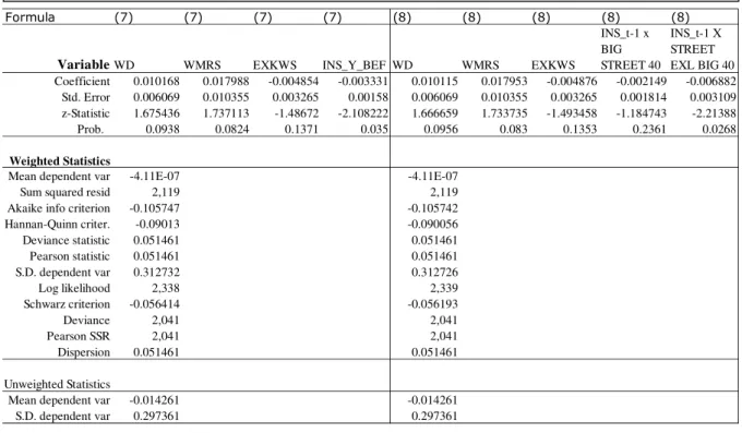
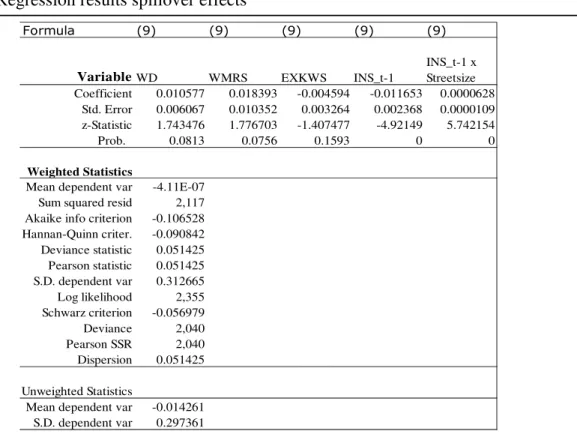
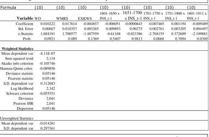
When analyzing spillover effects I find significant negative spillover effect of 0.3% from foreclosures to other properties in the same street. As the data allows to identify the location of properties on a street level, while having very long streets with over 600 properties in the sample, it is tested whether the street length influences the degree of the spillover effect. When analyzing the spillover effect in the 40 largest streets and in the rest of all streets, as a basic test which reflects the high skewness of properties per streets, I find a larger spillover effect [0.6%] in the smaller streets while spillover effects show a smaller economic magnitude [0.2%] and no statistical significance for the 40 largest streets. This is in line with previous findings of previous research which finds that spillover effects are a highly local phenomenon (Lin et al. 2009; Towe and Lawley 2013; Immergluck and Smith 2006; Harding et al. 2009; Munroe and Wilse-Samson 2013; Campbell et al. 2011). When quantifying this effect it can be seen that the spillover effects reduce per additional building in the street by 0.006%, hence the more buildings in the street, the smaller the spillover effects. As Li (2017) argued that spillover

(8)

5 effects are time variant, the same basic analysis of splitting the sample period into different sub-periods was applied in this thesis to identify potential time variation. The results of Li (2017) are confirmed insofar, that I find significant time variance in spillover effects. Furthermore, the spillover effects seem to be related to the general price development in the real estate market, as significant positive spillover effects co-occur with times of crisis in the residential property market.

A microdata level analysis reveals that many large investors in the real estate market refrained from purchasing properties in times of crisis and hence pulled out of the market, rather than buying foreclosed properties in large-scale. The same applies to people who are affected by large scale foreclosures, most people with large-scale foreclosures did not return to the real estate market despite being part of families with substantial wealth. Both groups are people which should be able to provide liquidity in a market which is distressed, as this is not happening a possible explanation for increasing foreclosure discounts and increasing spillover effects in times of crisis might be the structural change of the relationship between supply and demand. As the full sample period is characterized by a demand overhang due to the continuous population increase, the sudden removal of demand and creation of excess supply might have driven up foreclosure discounts and spillover effects, as an exact quantitative assessment is beyond the scope of that thesis this theory relies on descriptive statistics and is subject to further research.

The rest of the thesis is structured as follows: Chapter 2 will discuss the streams of literature which are affected by this thesis and develop the working hypothesis for this thesis. After that, chapter 3 will give an overview of the historical context and give an introduction to the procedural circumstances in the specific historic context. This is followed by chapter 4 which introduces the data used in this thesis and its unique characteristics. Chapter 5 will analyze foreclosure discounts over the full sample period via quantitative and qualitative methods, the finding will be extended in chapter 6 where the time variance of foreclosure discounts is investigated. To finish the analysis chapter 7 will investigate the presence and characteristics of spillover effects of foreclosures during the sample period. The chapters 5 to 7 all start with an explanation of the applied methodology and continue with the research results. In chapter 8 the results of the analysis part are contextualized and further discussed. The thesis will end with identifying the limitations of this thesis and the needs for further research before concluding this thesis.

(9)

6

2. _{Literature review}

Several streams of literature are affected by this thesis. While it is related to the current discussion of foreclosure discounts, this thesis also adds new academic findings to the assessment of spillover effects of discounts of foreclosed properties on neighboring properties. Lastly, this research adds to the understanding of real estate markets in a historical context.

2.1. Foreclosure discounts

This thesis is related to theoretical literature investigating the impact of foreclosures on real estate prices. The stream of literature investigating foreclosure discounts in real estate markets is widely accepted and is based on multiple quantitative studies of housing data. Pennington-Cross (2004) finds a foreclosure discount of 22% using a repeat sales methodology on US-housing data from 1995-1999. For Cleveland, Sumell (2009) finds a foreclosure discount of up to 50% for single-family houses. Campbell et al. (2011) find an average foreclosure discount of 27% relative to the value of the house, using a hedonic regression in a dataset of 1.8 million transactions in Massachusetts. They explain this discount as a cost of protection against vandalism risks, as houses are unprotected as they are likely to not inhabited. Zhou et al. (2015) find that foreclosure discounts are negatively related to recent house-price appreciation and find that high foreclosure discounts for lower value properties are likely due to property conditions. Clauretie and Daneshvary (2009) report in a comprehensive analysis a conditional foreclosure discount of less than 10% in data for Clark County, Nevada, between 2004 and 2007. They use a hedonic regression controlling for various property and neighborhood characteristics such as time on the market, cash sales and property condition.

Hardin and Wolverton (1996) extended the research focusing not exclusively on residential real estate but including income creating investment properties, they confirm the existence of foreclosure discounts in a magnitude of 22%. They argue that investors might be willing to accept discounts due to atypical seller motivations such as satisfying regulatory capital requirements, mitigating negative stock price effects or protecting credit ratings.

While most literature researches housing prices in the United States Donner et al. (2016) use data on sold apartments and single family homes from 2006 to 2013 in Stockholm, Sweden, to check via a hedonic spatial Durbin model for foreclosure discounts. They find a foreclosure discount of 20.1% for foreclosed apartments and 24.6% for foreclosed single-family houses and find in addition to that, that foreclosure discounts increase when the number of transactions

(10)

7 is limited. The second European sample, which is based on a universe of adult Danes in the period between 1990 and 2010 used by Andersen and Nielsen (2017). They conduct a natural experiment that reveals, that foreclosure discounts are larger in when house prices contract. The authors argue that the magnitude of discounts is related to the urgency of a sale, defined by the current market conditions and the financial situation of the seller.

In general, there seems to be a consensus about the existence of the default discount in recent literature but the reason behind this discount is continuously debated, one line of reasoning is that foreclosed properties, on average, are of lower quality as distressed owners of homes are less likely to maintain the property. This is confirmed by Clauretie and Daneshvary (2009) and Sumell (2009), who find that foreclosed homes with lower quality rating exhibit larger-than-average foreclosure discounts. Opposed to that, Harding et al. (2012) argue that the existence of a foreclosure discount would represent arbitrage opportunities and would hence allow purchasers of REOs [Real estate owned] to generate positive excess returns. They test this hypothesis by comparing the holding returns of REO buyers with those of buyers of similar properties that are not in financial distress and do not find significant excess returns for investors in distressed properties. Hence, they argue that the market for REOs operates efficiently and hence no arbitrage opportunity can exist which would, in fact, be an argument against the systematic existence of a foreclosure discount. This view is supported by Carroll et al. (1997), who comment in their paper the results of Forgey et al. (1994) and argue that the inclusion of ZIP-code dummies and common characteristics between foreclosed properties and their neighboring properties, causes the findings of significant foreclosure discounts between 12.18% and 13.96% to diminish to insignificant values between 0.17% and 2.59%. Consequently, Carroll et al. (1997) argue finding a significant foreclosure discount is the consequence of omitted variables in the statistical assessment rather than the existence of an economically significant discount.

This view is opposed by Aroul and Hansz (2014) who hypothesize that foreclosure discounts are dependent on house price volatility. Therefore the authors analyze foreclosure discounts in a sample of Fresno, California from 2006 to 2010, which due to the housing crisis in 2008 incorporates significant house price volatility. They find a 20% discount for foreclosure transactions which remains consistent when controlling for the endogeneity of time-on-the-market and self-selection bias. The magnitude of foreclosure discounts was challenged by Clauretie and Daneshvary (2009), who argue that, under the assumption of efficiency in real

(11)

8 estate markets, foreclosure discounts of 20% seem counterintuitive. The authors argue that findings that confirm foreclosure discounts of that magnitude are caused by an upward bias induced by omitted variables, they name the physical condition of the property and the relationship between marketing time and price as examples for such omitted variables.

Zhou et al. (2015) argue that the high variability in identified foreclosure discounts arises due to a lack of common definition of a foreclosure discount and subsequently define a foreclosure discount as the discount of the real estate owned (REO) sale price relative to a normal-sale estimated market value. They apply this definition on a dataset of 1.34 million REO sale transactions across 16 core-based statistical area (CBSAs) between 2000 and 2012 and find a significant foreclosure discount. Next, to that, they state three other empirical noteworthy findings, they find that a concentration of foreclosure sales increases the foreclosure discount, that foreclosure discounts are negatively related to recent house price appreciations and that high foreclosure discounts are often associated by houses of lower quality.

Summarizing it can be said that there seems to be a consensus about the fact that foreclosing properties sell at lower prices than properties which are not sold via foreclosures while there is an ongoing debate about whether this represents an arbitrage opportunity and is hence a market inefficiency or whether the lower sales price is inherent in the different conditions of foreclosed properties. This thesis tries to incorporate structural quality difference effects in the methodology and hence focuses on the explanation of foreclosure discount via a market inefficiency which might be explained by procedural uncertainty (Chinloy et al. 2017). In this context I use the similarity of foreclosure processes, namely having no right to inspect the property that is auctioned, having a remaining risk of additional claims on the property which are not addressed by the process of the execution remission and the fact that borrowers which foreclose are likely to have experienced a significant period of financial distress before foreclosing and hence might have neglected required maintenance on the property. To hypothesize that I will find a significant foreclosure discount throughout the full sample period, despite the earlier described procedural advantages of the Dutch-Anglo premium auction (Boerner et al. 2012). I believe that the quality effect, which might be driven by the financial situation of the owner, by for example delaying required maintenance, in combination with the lack of an inspection right and the remaining risk of additional claims on the auctioned property are dominating the effect of the advantageous procedural design of Anglo-Dutch premium auctions. This assumption is partly driven by the uncertainty of the range given by the

(12)

9 auctioneer, as the upper range is non-binding it might not significantly reduce the uncertainty when it is chosen very high. In addition to this main hypothesis I hypothesize to see time variation in foreclosure discounts, as the full sample covers multiple real estate cycles and Zhou et al. (2015) find a negative relation of foreclosure discounts to price appreciation in real estate markets I expect to see increasing foreclosure discounts in the times of economic crisis which materialized in a residential real estate crisis, for example, the period after the beginning of the Anglo-Dutch war in 1784 and the connected negative impacts on the economy. I do expect this time variation to be significant, as Amsterdam experienced during the sample period a large increase of inhabitants, as described by van der Woude (1982), this means that there has been very high demand for properties during the times of economic prosperity which is covered in the sample. As housing supply is limited and can only be extended gradually over time, I assume that the demand-overhang caused in many cases that the access to housing, irrespective of the procedural form of purchasing the property, was outweighing the previously described uncertainty associated with foreclosure sales. While this might have been valid in times of economic prosperity and inhabitants growth, this can not be assumed in times of economic crisis, as this limits the amount of potential real estate buyers and hence reduces or even reverts the demand overhang. In these times procedural uncertainties connected to the foreclosure process increase, as worsening economic conditions, also increase the risk of additional claims on the property as people might try to overcome seemingly temporary financial difficulties arising for example after a loss of a job, with additional credits where the own real estate is used as collateral. As in times of crisis, the effect of a demand overhang reduces and the risks associated with foreclosure sales increase, I hypothesize to find intra-sample time variance of foreclosure discounts which might be associated with the overall price development of the real estate market, as this seems to be a reasonable indicator for the prevalent supply-and-demand relationship.

2.2. Spillover effects of foreclosure discounts

The assumption that in many cases a contagion effect of foreclosure discounts on nearby properties exists is researched in the second stream of literature which relates to this thesis. Here analyzing co-movements of Case‐Shiller Home Price Indices for 14 metropolitan areas in the United States between 1992 and 2008 Kallberg et al. (2014) find that the co-movements, which are not attributable to the fundamental factors that determine real estate prices, are increasing over time. They argue that this increase can be explained mainly by the underlying

(13)

10 systematic real and financial factors and that this would be consistent with a greater fundamental integration of these markets. But the authors also argue that the existing excess co-movements are a less important factor for structural housing prices than commonly believed. Immergluck and Smith (2006) find in a dataset of more than 9,600 property transactions in Chicago in 1999 that foreclosures within an eighth of a mile of a single‐family home result in a decline of 0.9% in value of the home which has not been foreclosed. In the same line of research Harding et al. (2009) find that evidence of a contagion discount of roughly 1% per nearby foreclosed property by simultaneously estimating the local price trend and the incremental price impact of nearby foreclosures. They also find a high local dependency, via strong decreases in contagions discounts, when the distance to the foreclosed property is increased.

Lin et al. (2009) find that spillover effects of a foreclosure on neighborhood property values depend on two factors: the discount of foreclosure sale and similarity of the property that was foreclosed to the property that is sold, as these factors drive the inclusion of a transaction in the valuation multiple. Their empirical analysis identified a radius of 0.9 kilometers [km] in which foreclosed properties cause contagion discounts while these discounts show a declining persistence over 5 years. In their sample, the most severe contagion discount is 8.7% discount, which gradually drops to anywhere between 1.7% to 4.7% over the time period of up to 5 years after the liquidation sale.

Arguing that most previous research on spillover effects of foreclosure discounts on non-distressed house sales are based on samples from stable housing market periods, Daneshvary et al. (2011) use transactions for 2008 from a housing market with a relatively large number of REO sales and foreclosures. They find that REOs and foreclosures have the same spillover effects and quantify this effect at 1%. Consequently, they analyzed that the total cumulative effect of distressed neighbors can cause a loss of value on a neighboring property of up to 8%. When distressed sales are excluded from this estimation the marginal spillover effect increases to 2% and the maximum cumulative effect in the sample increases to about 21%.

This is in line with the research of Li (2017), who finds a negative effect on property prices is significant from nearby foreclosures, real estate owned (REO) listings and REO sales, but not from default and delinquent properties. She also states that there is time-variation in terms of having a larger effect in depressed markets and a smaller effect in appreciating markets. The author argues that the most plausible explanation for the spillover effect is a depression of the

(14)

11 associated reference prices. By disentangling the effect of changed supply and dis-amenity stemming from deferred maintenance or vacancy of neighboring properties Hartley (2014) wants to isolate the cause for spillover effects in the neighborhood. The author finds that the effect of dis-amenity is close to zero while each extra unit of supply decreases prices within 0.05 miles by about 1.2%, which is in line with the magnitude of previously measured spillover effects. Extending the research to measuring not only the impact of a neighboring foreclosure and REO process but including the duration of such an impact Zhang et al. (2015) find a negative neighborhood effect, measured by the negative externalities resulting of neighboring foreclosure and REO processes when extending the length of the foreclosure process.

Towe and Lawley (2013) extend their research beyond quantifying the effect of foreclosures on neighboring property values and hypothesize that foreclosures have an impact on the foreclosure likelihood of neighboring property and this implies a negative social multiplier effect of foreclosures on neighborhoods. They do find that a neighbor foreclosure increased the likelihood of additional defaults within the neighborhood by 18%. This is in line with the findings of Munroe and Wilse-Samson (2013), who find that completed foreclosures cause between 0.5 and 0.7 additional filings within 0.1 miles and argue that learning plays an important role in contagion, rather than the pecuniary externality of the neighboring foreclosure, as the contagion effect is largely driven by borrowers which are not facing the immediate threat of default.

Analyzing the implications and dynamics in “hard-hit” neighborhoods in New York City and the core counties of Atlanta and Miami, Ellen et al. (2014) find that the most affected regions measured by the relative occurrence of REOs do not show characteristics of being the poorest or having the highest unemployment rates. They also do not find that investors do account for a significantly higher proportion of purchasers of REO properties in the hardest-hit neighborhoods than in other neighborhoods.

While there seems to be a general consensus on the fact that foreclosures do have an impact on their neighborhood, Calomiris et al. (2012) argue that the association, which can be observed between non-distressed house prices and foreclosures, is mostly driven by the endogenous adjustment of foreclosures to prices via the strategic choices of homeowners and lenders and not through the effects of foreclosures on home prices. The authors base this argument on a panel VAR, including macroeconomic and housing variables such as employment, permits or sales, using quarterly state‐level data from 1981 until 2009. They find a dominating

(15)

12 relationship where prices have a much larger impact on foreclosures than vice versa. Summarizing the literature of spillover effects from foreclosures, recent literature finds that the spillover phenomenon is a highly local effect which decreases with increasing distance to the property, when it comes to explaining the spillover effect the main theories are that prices which are used for comparison are influenced by a property which foreclosed and possibly was sold at a discount or that a lack of maintenance on foreclosed properties damaged the neighboring properties by diminishing the appearance of the neighborhood (Harding et al. 2009) or that changes in supply cause the spillover effect (Hartley 2014). Another explanation is the inclusion of foreclosed properties when assessing the value of a nearby property, under the assumption that the foreclosed property transaction was processed at a discount (Lin et al. 2009). As little is known about value assessments of property in the 16th_{to 19}th_{century in}

Amsterdam, but the conditions of deteriorating neighborhood appearances as a consequence of lack of incentivization and lack of financial resources to maintain the property and the effect of supply changes should be present in a historical setting, significant spillover effects are expected throughout the full sample period. This can be supported when foreclosure sales are seen as sales which involuntarily add supply to a market in an unideal moment market. Hence these transactions create market imbalances via creating excess supply, relative to the normal supply level which characterizes a respective period. That materializes in changed supply-and-demand relationships that consequently change the price for properties that are similar in terms of fundamental characteristics and location. Consequently, I expect strong time variance of these effects with an increase in spillover effects, when demand is limited by for example worsening economic conditions and changes in supply directly materialize changes in price and are not masked by excess demand, this hypothesis is in line with the argumentation of Li (2017).

3. _{Historical Background}

This section will provide the general historical background of Amsterdam for the studied period and discuss the general structure of the housing market in Amsterdam and the procedural requirements for the acquisition of houses during the sample period. This description is complemented by an introduction into the legal proceedings following a default of creditors in the context of real estate credits. In addition to that, I will introduce the Anglo-Dutch premium auction as the auction mechanism of foreclosure sales and compare this mechanism with the currently prevalent form of foreclosure auctions.

(16)

13

3.1. Amsterdam in the 17th and 18th century

The studied period from 1509 until 1811 covers the rise of the Netherlands to European economic leadership, the Dutch Golden Age and the subsequent decline of the Dutch economy. During that time Amsterdam played a central role for the Dutch economy and became a global trade capital, but the time period also covers Amsterdam’s decline of importance as trade capital, due to the emergence of competitors like London and the German North Sea ports. The book of de Vries and van der Woude (2007) describes the development of the Dutch economy from 1500 until 1815 and serves as the main source of information for the remainder of this section.

Amsterdam had an important role as a driver of the Dutch economy due to its role as European trade hub which hosted at its heights more than half of Europe’s total merchant marine capacity (Blanning 2008). In the late 16th_{and 17}th_{century Amsterdam accumulated rapidly trade capital}

from merchants outside of the Dutch Republic. High-risk ventures like revolutionary expeditions to the lands of South and Southeast Asia attracted those merchants and were soon incorporated into the Dutch East India Company (VOC). The success of the VOC can be seen in the enormous profits and the expansion of the fleet from 827 ships before 1610 to 3049 ships between 1650 and 1660 (Parthesius 2010), which not only illustrates the economic success of those ventures but also the importance of Amsterdam for the global trade activities. This economic success led to fast pace population growth and strong urbanization, defined as population increase in cities is higher than the population increase in rural areas. This materialized in an increase from 150 thousand inhabitants in urban areas in the region of Holland in 1550 to approximately 400 thousand inhabitants in urban areas in the same region in 1650 (van der Woude 1982). Given the aerial limitations in Amsterdam, several expansion projects were required (Abrahamse 2010) to satisfy the increased need for housing in Amsterdam. In the 1650s the boom period reached its zenith with an overall productivity, which was the highest in Europe at the time and has been reflected in the high wage level of the Netherlands during that period.

However, two mutually reinforcing economic trends ended the boom period in the Dutch Republic. The closure of major European markets as a consequence of the second Anglo-Dutch war, Dutch-Swedish War and the Franco-Dutch War and the associated protectionist measures which the European countries took, led to an end of the increases in trade volumes for the Dutch economy. In isolation, the effect of reduced trade volume growth would probably not

(17)

14 have been so severe, but at the same time the continuous trend of rising price levels had reversed from inflation to deflation. Due to the stickiness of nominal wages in economic downturns (Bernanke and Carey 1996) real wages continued to rise, despite the economic downturn. Both reinforcing trends led to a substantial economic downturn and stopped the fourth expansion of the city of Amsterdam (Abrahamse 2010).

Despite this severe economic downturn, the economy of Amsterdam managed to recover during the late 17th_{and early 18}th_{century. Amsterdam remained a wealthy city and repositioned}

itself as a leading financial center, in close cooperation with London. During the 18th_century

the population of Amsterdam remained at a constant level and consequently, there have been little changes in the housing stock. The period of political neutrality which characterized the 18th_{century of the Netherlands came to an end in 1780 with the start of the fourth Anglo-Dutch}

war. This marked also the end of wealth for Amsterdam, which was taken over entirely by the French in 1795 (de Vries and van der Woude 2007).

3.2. The housing market and procedural requirements for property transactions in Amsterdam

The economic importance of Amsterdam during the sample period and the consequential rise of the population in Amsterdam indicate the important role of the housing market in Amsterdam. Korevaar (2018) used the same archival data that is used in this thesis to discuss the structure of the housing market in Amsterdam and analyzes four features of the housing market. The description of the housing market and the introduction to procedural requirements for acquiring real estate during the 16th_{and 17}th_{are mainly based on his work, the work of (van}

Bochove et al. 2015) and is complemented by additional research in this area.

Every transaction of real estate had to ratified and registered in front of the aldermen of Amsterdam (schepenen). Auctions or alternative forms of transfer organizations were possible but did not exempt buyer and seller from the duty to register the transfer with the alderman to initiate the formal transfer of ownership. The registration of property transfers was a requirement all over the Dutch Republic and was administered at the municipality level. The oldest available register for Amsterdam stems from 1563 and the latest transaction was registered in 1811.

(18)

15 Regular property sales were recorded in an act of ordinary remission (ordinaris kwijtschelding) that followed a standard format, as shown in the transcribed example in appendix A, that is taken from Korevaar (2018), which describes a transaction of the famous painter Rembrandt

The text shows, that the sellers’ name and the buyers’ name are mentioned and that the buyer had to bring two guarantors for the transfer. In addition, it becomes apparent that buyer or seller that could not legally represent themselves, such as died homeowners, women and children, had to be represented by guardians, which were usually close family members. Furthermore, details about the purchased object are described in a way which should ensure the correct identification of the transferred object. This description included the property itself but also the location. This is important as homes were not numbered in during the sample period and the location was identified based on the street name, points of interest or the owners of houses nearby. Additionally, the data set reveals that house prices are only recorded from 1637 onwards and while it was common to have multiple sellers, it was less common to have multiple buyers, which could be explained by the fact that many transactions with multiple sellers name the heirs of the original owner.Next to regular sales (ordinary remission) there were additional forms of property transfers. When a homeowner defaulted on a loan, which were always full recourse loans in the Dutch Republic during the time of the sample period, the possessed property could be auctioned off by the creditors via the city of Amsterdam, the exact process is described in the following chapter.

As Amsterdam had a large market for private credit it was possible that creditors had claims on a property although the debtor sold the property off. This was generally limited to a time period of 1 year. In case an acquirer of a house wanted to ensure that no creditor had a remaining right on the property which was acquired, the seller and buyer had to possibility to transact the property via a willig decreet at the court of Holland (van Iterson 1939). During that process, the acquisition was made public three times in 14-day intervals, which allowed creditors to make a claim and settle the debt. After that procedure, the creditor had no rights anymore on the property and had to settle the credit with the debtor without the initial security. Korevaar (2018) notes that this process was often used when there was significant doubt about the fact whether all credits have been repaid by the seller, as he finds a close correlation between the number of willig decreeten and the number of foreclosure sales. A similar process existed for foreclosure sales, these transactions were named onwillig decreeten and followed the same process with the same underlying reasons, with having a foreclosed property being

(19)

16 transacted.Another possibility was the transfer of property via the orphan chamber (weeskamer), the orphan chamber had the legal authority to register all transactions with a relation to the property of orphans in the books of orphan guard auctions (weesmeesterverkopingen), hence these transactions were not registered with the aldermen.

3.3. Defaults and other market dynamics in the housing market of Amsterdam

When a homeowner defaulted on the payments agreed upon in the mortgage agreement in Amsterdam in the 16th and 17th century there were three legal ways in which the property was transferred which are similar to modern foreclosure sales. The most used form was the transfer via an execution remission (executie kwijschelding), in this process the bailiff of Amsterdam would seize the assets of the debtor for the creditor, here it was common that the debtor had a possibility to pay the debt and subsequently avoid the seizure of his assets. When the asset was seized by the bailiff the debtor could request a letter from the aldermen, granting the permission for the auctioning of the seized asset. This was usually done via public auctions organized by the city of Amsterdam. After the auction, the transfer of ownership was directly registered with the aldermen as an execution remission (executie kwijschelding). This form of defaults shows significant similarities to the organization of foreclosure sales today. Boerner et al. (2012) describe an the Anglo-Dutch auction process which represents the auction process used during the 18th and 18th century in Amsterdam. An Anglo-Dutch premium auction constituted of two possible rounds of bidding. In the first round, bidders bid against each other with ascending prices as in a standard English auction, the highest bidder of the first round would receive a pre-determined cash prize (premium), regardless of the outcome of the second round. In the second round, the auctioneer would set a high price and call out decreasing prices if somebody was willing to bid a price between the high price and the highest price of the first round that person would win the auctioned object, hence everybody could participate in the second round. If no bid was made in the second round the winner of the first round would win the object. The earliest auctions following that process are documented in 1529 and were used throughout the Dutch Republic in the 18th and 19th century to sell real estate and other goods. Today there are two main forms of foreclosures: judicial foreclosure, which requires the creditor to go to court and receive a judge’s approval to foreclose a property and nonjudicial foreclosure, where the creditor may sell the property or repossesses it without a judge’s approval (Enoch et al. 2014). When looking at the process of judicial foreclosures today, as described for the state of Florida by Shneyerov et al. (2015), one can see that when the borrower defaults the court grants

(20)

17 the lender, upon specific request of the lender, a right to foreclose a property. After that, the lender is allowed to auction the property off to the highest bidder, in general via English auctions. While the title is transferred to the highest bidder, certain liens and encumbrances may survive the foreclosure sale. It is the obligation of the bidder to find out about these liens and encumbrances, which creates a high level of uncertainty. This uncertainty is increased by the fact that no “open houses” will be held, hence the bidder does not have the right to inspect the property before engaging in the auction. Similarly to the Anglo-Dutch process, it is common that the lender makes a bid for the property, which can be seen as reserve price and sets a lower price boundary previous to the auction process.

When comparing both processes we can identify interesting similarities and differences, which might have implications on the efficiency of the full process. In both processes, the acquirer of the foreclosed property is exposed to the risk of a remaining claim on the property, which could only be remedied during the sample period via onwillig decreeten or willig decreeten at the court of Holland as described before. When looking at the auction process it becomes apparent that the uncertainty remains high in both procedures due to the limited inspection rights, but the design of the Anglo-Dutch auction seems to be beneficial in terms of uncertainty as it determines lower and upper boundaries before entering in the final bidding stage, while auctions today just set lower boundaries by the bid of the lender. This is confirmed by the empirical findings of Boerner et al. (2012), who find a positive empirical connection between greater uncertainty in the security’s value and a greater likelihood of a second-stage bid, which exhibits the characteristics of having upper and lower value boundaries. The authors state that this particular auction design solved a complex market problem and led to efficient auction prices. In the context of foreclosure discounts, the unique process design during the sample period might have reduced procedural uncertainty and hence reduced one explanatory factor for structural foreclosure discounts.

Mian et al. (2015) describe that institutions and regulations of foreclosure processes have implications on the likelihood of foreclosing a property and hence have implications for the change of housing supply in the market. This might lead to changing market dynamics with changes in regulation and hence would have to be reflected in the econometric method. This concern is remedied by the fact that the institutions and processes remain constant within the full sample, despite having a time-variant share on total transactions.

(21)

18

4. _Data

The initial dataset “transportakten” from the Amsterdam City Archives consisted of 164,047 real estate transactions in Amsterdam and its surroundings from 1509 until 1811. The dataset constituted of the transaction ID to identify the transaction, sub-transaction ID to distinguish between potential multiple buyers and sellers, property ID to identify the property which was transacted. Additionally, the data includes a series, which identified the legal transfer procedure, for example, obedient court orders or execution remission. The transactions are further described by the date of the transfer, the purchase price of the transaction, the full name of all involved buyers and sellers or their potential legal representatives, in case of legal representation the data provides the reason for the requirement of legal representation. The location of the transacted property is defined by the place of the location for example “Amsterdam”, the street name of the real estate, the original street name, the name of the house, if applicable and the position of the property for example “over het Boshuis” (over the forest house). Additional variables identified the nature of the transacted good, the data distinguishes between for example between house, land, rear house, garden, warehouse, workshop and 18 more subcategories which help to understand the nature of the transacted property. In total the dataset has 84 variables across 164,047 transactions with 454,680 entries.

The dataset was transformed for the necessary analysis in this thesis. In order to clean the dataset, the following restrictions were given for each subsample. Every transaction was included once, when a transaction was recorded multiple time e.g. when multiple sellers sold one house only the first seller was included in the dataset. As a next step all transactions that did not take place in Amsterdam were excluded, here a very strict approach was applied, excluding every transaction that did not have “Amsterdam” as an entry for the variable “Plaats” (place), in order to avoid noise from different pricing dynamics outside of Amsterdam. As a fourth step, every transaction that did not include a house was excluded, this was done via using the dummy variable “huis” (house) as a filter, this limits the sample to residential real estate. As a next step houses that were transacted for a price of zero or where no price was given were excluded, as prices of zero should not represent a market-driven price building for a house with an intrinsic value that should be higher than zero in any case. Usually, prices of zero are given in the sample when the price cannot be seen in the record of the transaction. To control for double entries a control variable was created by combining the date of the transaction, the property ID and the “bedraag” (price). This variable was filtered for double

(22)

19 entries. As all previously described data adjustments were done using automated tools in excel, the resulting datasets were checked manually for double entries and merged into one dataset.

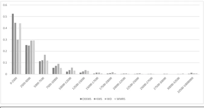
In a lengthy manual process, matches were built, these matches are based on the property ID and the corresponding date. Every time a property was transacted more than two times in the total dataset the multiple matched transactions were recorded to measure the change in price for every additional transaction. Additionally, a variable measuring the log price change between the first and second sale was created and a variable measuring the time difference between the first and the second transaction in years. To measure the impact of insolvencies on street level one variable was created, the variable is a count of insolvencies, defined as sales via execution remissions in the same street in the year, preceding the recorded transaction. The final transformed dataset consists of 62,797 residential transactions with prices and 316 variables, of which 230 were newly created, the summary statistics of the most important variables can be found in in appendix B. When calculating returns for the matches, while including multiple transactions of the same property by calculating the returns between each known transaction, one finds 39,893 returns based on the previously identified matches. When looking at the different price distributions, we can see that all kinds of transactions show a heavy right skewness (figure 1). Campbell et al. (2011) found in their research the same characteristic right skewness of foreclosure sales, which is prevalent in the dataset used in this thesis, with having most foreclosure sales between the value of 15 to 9,115 Gulden but having a very long tail with the largest foreclosure sale of 103,000 Gulden. In total the dataset consists of 5,330 sales via execution remission, which represents 8.49% of all transactions in the sample.

It can be seen that execution remissions are more concentrated in the extremes, as one can see that the share of transactions within the highest and lowest transaction value bracket is higher than the share of transactions within these value brackets of all other forms of transactions. When comparing the distribution of foreclosure sales and normal sales, one can see that foreclosure sales are much more concentrated in the low-value bracket than normal sales. That confirms previous findings that foreclosures concentrate on low-value properties (Li 2017), while this makes intuitive sense, as people who purchase residential real estate that is cheaper might often have lower income and fewer savings and hence are more exposed to changes in income and consequently the economic conditions. The higher concentration of foreclosure transactions in very high property value real estate’s is puzzling. It might be explained through

(23)

20 the smaller amount of foreclosure sale transactions, and an unusual high amount of rare high-value property foreclosures. This seems unlikely though through the length of the total sample. Another reason might be the emergence of financial products and the financing of high-risk ventures via financial products, here a later example will show thatmembers of very wealthy families engaged in high-risk business ventures and eventually defaulted after longer periods of financial struggle defaulted on a massive scale. This period specific phenomenon might explain this above-average concentration of foreclosure sales in high the value bracket.

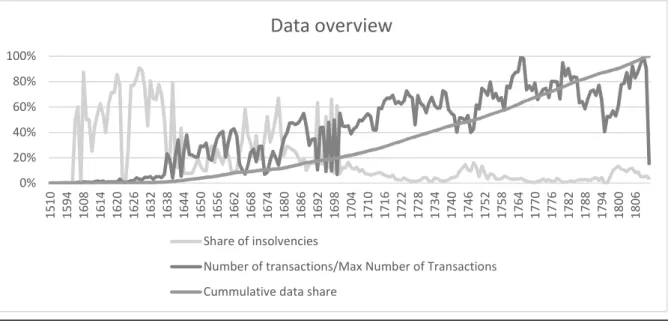
In terms of data quality one can see that the data until 1644 is very limited, often with less than 100 transactions per year but after 1644 the data quality improves significantly with an average number of 167 transactions and a maximum of 683 transactions in 1765. This might be driven by the share of registers that are preserved until today but seems relevant in terms of conclusions that can be drawn on data preceding 1644. Looking at the share of insolvencies per year one can see that the share of insolvencies increases when the share of transactions decreases (figure 2), this is driven by a decrease in absolute transactions combined with an increase of absolute foreclosures. Figure 2 and figure 3 also reflect the cycles in the real estate market of Amsterdam, from 1700 one can identify 2 major periods of crisis in the residential real estate market when looking at the share of insolvencies relative to yearly transactions. The first crisis after 1700 seems to occur around 1740, this co-occurs with a lengthy recession described by de Vries and van der Woude (2007). The second major real estate crisis can be seen after 1794 which was during the fourth Anglo-Dutch war and the connected detrimental

(24)

21 effects on European trade, which severely harmed the Dutch economy during that period. These crises are also reflected in the price development, when plotting median prices, to avoid the noises of averages, we can see that the real estate crises, that have been identified using the share of foreclosure sales on total sales, co-occur with the end of continued real estate price declines. In addition to that, we can see the tendency of foreclosure sales to be concentrated at the extremes of price ranges during a period due to the high standard deviation of median forced prices when comparing them to the median unforced prices (figure 3).

0% 20% 40% 60% 80% 100% 1510 1594 1608 1614 1620 1626 1632 1638 1644 1650 1656 1662 1668 1674 1680 1686 1692 1698 1704 1710 1716 1722 1728 1734 1740 1746 1752 1758 1764 1770 1776 1782 1788 1794 1800 1806

Data overview

Share of insolvencies

Number of transactions/Max Number of Transactions Cummulative data share

Figure 2: Overview transactions and insolvencies per year & data distribution over the sample period

(25)

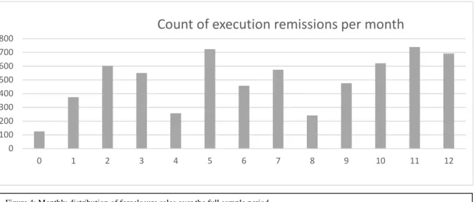
22 To analyze whether the different distribution of foreclosure sales might be procedurally induced by for example a monthly concentration of foreclosure auctions which would expose foreclosure sales to other monthly effects than regular sales, the distribution of monthly occurrence of foreclosure sales was plotted in figure 4. This distribution reveals that foreclosure auctions have not been taken place in specific months as no monthly concentration can be found in the data. Hence we cannot explain the higher standard deviation or the higher skewness of foreclosure prices via monthly effects or sales concentrations that might have affected the purchase behavior of real estate investors and homeowners.

When looking at further variables present in the dataset one can draw interesting conclusions on individual investor behavior during the sample period, which can be used to describe and explain the previously described characteristic of the real estate market and certain sub-dynamics within the residential real estate market especially in times before and after foreclosures or crises, for that purpose two samples were created.

The first sample is a list of the 50 persons with the highest accumulated value of default transactions as a seller. The 50 largest sales from execution remissions accumulate to 1,915,462 Gulden, have an average transaction value of 38,309 and a median transaction value 34,100 which reconfirms the right skewness of execution remissions. At a later stage, this data will be used to gain a deeper understanding of what kind of people foreclosed large amounts, what they foreclosed and how the process affected their behavior in the overall market.

The second sample identifies a residential real estate market crisis from 1743 to 1751, this seems surprising as de Vries and van der Woude (2007) find that in 1742 the per capita GDP (Gross domestic product) was at was at the end of a long period of decline after the economic

Figure 4: Monthly distribution of foreclosure sales over the full sample period

0 100 200 300 400 500 600 700 800 0 1 2 3 4 5 6 7 8 9 10 11 12

(26)

23 peak of 1650 this means that the crisis, defined by the above average share of insolvencies on total transactions, co-occurs with an economic upswing. A period of ten years before and ten years after the crisis is defined and used to identify structural changes, like the average transaction price but also use the data to identify the most active people in the residential real estate market before and after the crisis and see how the behavior changed.

5. _{Non-time variant foreclosure discounts}

5.1. Methodology

In order to identify foreclosure discounts in the samples an extended repeat-sales methodology is used, which is based on Bailey et al. (1963) and Case and Shiller (1987). This was done to reflect the nature of the dataset, that despite the sample size has little to no data which could be used in a hedonic regression opposed to the dataset that is used by Immergluck and Smith (2006). In addition to that Harding et al. (2009) argue that the repeat sales approach substantially reduced the omitted variable problem of hedonic models and is compatible to identify separate effects of the overall price trend.

The model is based on the standard repeat sales model and extends it by a term for the transaction type. It defines that a transaction price of a home i in a year t can be separated in the following characteristics:

!_"# = %_" + '_"+ (_#+ *_"# (1)

%_" represents the quality of a home and is assumed to be time invariant. '_" represents dummies

for the type of sale and (_#represents the monthly seasonality while *_"# captures remaining transaction noise. Korevaar (2018) used additionally the term +# to capture the current level of

market prices via an interest rate parameter. Taking log differences, the return of a home i between time t and s can be written as follows:

,"#− ,". = /"# − /".+ 0#− 0.+ 1"#− 1"., 3 < 5, 1~7(0, :;) (2)

The equation gets estimated for all pairs using OLS, where the time period in years, the type of sale and the transaction month are identified by dummy variables for each period, type or month. In order to reflect the nature of differencing, the dummy variables take the value one in period t and the value minus one in periods. Regular sales in January 1510 are taken as the

(27)

24 baseline for further estimations. Heteroskedasticity, which might arise through holding period differences, is controlled via the Case and Shiller (1987) adjustment, this is done for every regression that is based on a repeat sales approach in this thesis.

To address the concern that the combination of foreclosure sales drive foreclosure discounts, consequently that investors who buy houses from foreclosures to sell them via normal sales procedures and profit from that behavior, a set of dummies was created that controls for the different possibilities of including execution remissions in a transaction. While the standard model would identify two consecutive foreclosure sales as zero in the variable for foreclosure sales, I explicitly model this opportunity as a dummy which is one if both sales are foreclosure sales and zero if they are not, in the same way, the other two opportunities are modeled.

,"#− ,". = =".>3"#+ >3".&"#+ ="#>3". + / "#− / ".+ 0#− 0.+ 1"#− 1".,

3 < 5, 1~7(0, :;₎ ₍₃₎

,where =". represents a not forced sale, >3"# represents a forced sale and the combination from

both [=".>3"# and ="#>3".] represent in accordance to the time periods the different points in

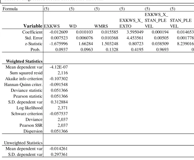
time and / represents the dummies for the remaining transaction forms. This leads to a clear identification of the impact of each possible combination on the price difference. From these combinations, I can draw conclusions on the quality of a home, by the realization of premiums or discounts in every possible combination. When I am able to realize structural premiums by acquiring foreclosed properties and selling them via normal sales procedures an explanation of the foreclosure effect by fundamentally worse quality is unlikely because when quality is discounted in a foreclosure process it should be discounted in a normal sales process, too. Hence no premium should be realized in this combination.

This procedure is supported by a microdata level analysis that covers the behavior of investors before and after the residential real estate market crisis from 1743 to 1751. Therefore investors were listed and ranked based on their transaction activity within 10 years after the end of the crisis in 1751. The behavior was analyzed analog to the analysis that was done for the people with the highest foreclosing values, for the 20 most active market participants measured by an absolute count of sales in the period after the crisis. This analysis offers interesting insights on whether the most active real estate investors used foreclosure sales to generate returns by

(28)

25 buying via foreclosure sales in the crisis and selling of the acquired assets after crisis via normal sales procedures to maximize profits.

5.2. Results

In table 1 one can see the results of the adjusted repeat sales regressions. Interestingly enough one can see that over the full sample period no significant foreclosure discount can be found.

This implies high market efficiency in the real estate market of Amsterdam during that time period. The overall results are in line with Harding et al. (2012) who state that the existence of a structural foreclosure discount would represent an arbitrage opportunity. This also confirms the findings of Boerner et al. (2012) who find that the Anglo-Dutch premium auction solves a

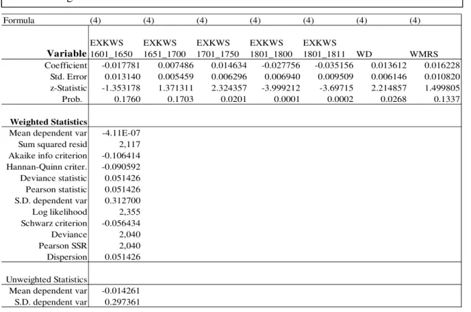
Table 1: Regression results foreclosure discount

Formula 2: ,"#− ,".= /"#− /".+ 0#− 0.+ 1"#− 1"., 3 < 5, 1~7(0, :;_{), with EXKWS being the transaction type}

dummy for foreclosure sales, WD being the transaction type dummy for willige decreeten and WMRS being the dummy for orphan sales. Not reported here are all yearly and monthly dummies, as they are control variables.

Formula 3: ,"#− ,".= =".>3"#+ >3".&"#+ ="#>3". + / "#− / ".+ 0#− 0.+ 1"#− 1"., 3 < 5, 1~7(0, :;), with

EXKWS_1 NORM_2 being the dummy for houses that were purchased via foreclosure sales and sold via normal sales, EXKWS BOTH being the dummy for houses that were bought and sold via foreclosure sales and NORM_1 EXKWS_2 Being the dummy for houses that were bought via normal sales procedures and sold via foreclosure sales. Not reported here are all yearly and monthly dummies, as they are control variables. Both regression results present the result after the Case and Shiller (1987) adjustment for heteroskedasticity.

Formula (2) (2) (2) (3) (3) (3) (3) (3) VariableEXKWS WD WMRS WD WMRS EXKWS_1 NORM_2 EXKWS BOTH NORM_1_ EXKWS_2 Coefficient -0.004713 0.010373 0.017998 0.010353 0.018285 -0.012231 0.000450 -0.012027 Std. Error 0.003264 0.006069 0.010355 0.006069 0.010361 0.005414 0.004054 0.013331 z-Statistic -1.444059 1.709354 1.738013 1.705904 1.764836 -2.258987 0.111106 -0.902201 Prob. 0.1487 0.0874 0.0822 0.0880 0.0776 0.0239 0.9115 0.3669 Weighted Statistics

Mean dependent var -4.11E-07 -4.11E-07

Sum squared resid 2,119 2,119

Akaike info criterion -0.105685 -0.105680

Hannan-Quinn criter. -0.090136 -0.089994 Deviance statistic 0.051464 0.051462 Pearson statistic 0.051464 0.051462 S.D. dependent var 0.312756 0.312746 Log likelihood 2,336 2,338 Schwarz criterion -0.056567 -0.056131 Deviance 2,041 2,041 Pearson SSR 2,041 2,041 Dispersion 0.051464 0.051462 Unweighted Statistics

Mean dependent var -0.014261 -0.014261