A Work Project presented as part of the requirements for the Award of a Master
Degree in Finance from the NOVA
–
School of Business and Economics.
DYNAMIC RETURNS OF BETA ARBITRAGE
MAFALDA CORREIA MARTINS NASCIMENTO, 2284
Project carried out on the Master in Finance Program, under the supervision of:
Professor Afonso Eça
2
Dynamic Returns of Beta Arbitrage
Abstract
This thesis studies the patterns of the abnormal returns of the beta strategy. The topic
can be helpful for professional investors, who intend to achieve a better performance in their
portfolios. Following the methodology of Lou, Polk, & Huang (2016), the COBAR measure is
computed in order to determine the levels of beta arbitrage in the market in each point in time.
It is argued that beta arbitrage activity can have impact on the returns of the beta strategy. In
fact, it is demonstrated that for very high levels of arbitrage in the market, the abnormal
returns become negative.
3
1. Introduction
The linear relationship between beta and return developed by Sharpe (1964) and
Lintner (1965) described in the CAPM was thrown apart by several contemporary authors
who disagree that beta is the only risk factor explaining securities’ returns. Black (1972) was
the first in line with the study of the beta anomaly. He was able to find empirical evidence
that the security market line presented in the CAPM was too flat on average. Other authors
added that the empirical results were particularly evident in periods of high expected
Inflation, shown by Cohen, Polk & Vuolteenaho (2005), high Disagreement of investors
regarding the expected return of the market, publicized by Hong & Sraer (2014), and
investors’ Sentiment, demonstrated by Antoniou, Doukas & Subrahmanyam (2013).
The impact on asset prices by arbitrageurs has been a long discussion, started by
Keynes (1936) and Hayek (1945). It has been argued that arbitrage activity can contribute to
market efficiency, defended by Friedman (1966). Others, such as Stein J. C. (1987), argued
that it can have the opposite effect and push the prices away from their fundamentals. A third
perspective defended by Lakonishok, Shleifer, & Vishny (1992) claims that the market is
composed of investors with different views and goals that come together and offset each
other. The aim of this thesis is to understand the role of arbitrage activity in the returns of
investors who pursue beta arbitrage. Measuring such activity has been proved to be
challenging, but recently Lou & Polk (2014), inspired by the comovement of stock prices
presenting specific characteristics showed by Barberis & Shleifer (2003), developed the
Comomentum which measures the outcome of the arbitrage process, by observing the
correlation of price impacts. The principle behind this measure is the following: when
arbitrageurs take a position on assets, their trades can have simultaneous impacts on prices,
4 Lou, Polk, & Huang (2016) continued their previous study (Lou & Polk (2014)) to
develop the measure COBAR for the comovement of stocks in the beta strategy. High (low)
values of COBAR identify high (low) amounts invested in beta strategy. The aim of this thesis
is to further develop the study of the COBAR measure, following and questioning the
methodology used by Lou, Polk, & Huang (2016), and to better understand the impacts of
arbitrage on the returns of the beta strategy.
In the first part of the thesis, the COBAR measure of Lou, Polk, & Huang (2016) is
replicated. Additionally, the computation of COBAR is performed under different
specifications, with the aim of understanding which specification of COBAR can measure beta
arbitrage activity more accurately. The specifications are related to the Asset Price Model
defined for the estimation of residuals, the decile of stocks used for the calculation of the
measure and the exclusion of penny stocks from the sample.
In the second part of the thesis, the main findings of Lou, Polk, & Huang (2016) are
questioned: when levels of beta-arbitrage are low, the returns of the strategy take longer to be
realized and when the levels are higher, the returns are collected in a shorter term. When
arbitrage activity is more crowded (measured by the 20% of the sample with higher values of
COBAR) the abnormal returns of the strategy are recognized within the first six months. On
the contrary, when arbitrage activity is low (measured by the 20% of the sample with higher
values of COBAR), the returns take around 3 years to materialize. An understanding of what
happens to the returns of the strategies after the 3 years period (until 5 years) will be added
with the goal of having a long-run perspective of the relations explained above. The returns
are created using the CAPM, 3 factors-, 4 factors-, 5 factors- and 6 factors Model to ensure
consistency in the results observed.
In order to scrutinize the topic with more detail, some empirical evidence showed by
5 the behavior of the beta strategy returns described above is more pronounced in the presence
of relatively more leveraged stocks. The betting against beta strategy described by Frazzini &
Pedersen (2014) can be associated with positive-feedback trading. In fact, as it has been
characterized, it is difficult for investors to know how much beta arbitrage is being performed
in the market. If an investor bets successfully on low-beta stocks, the price of the stock will
rise. If the stock belongs to a company with relatively high levels of leverage, the increase in
the price will cause the beta of the security to decrease even more. The leverage consideration
is defined by Proposition II of Modigliani & Miller (1958). It claims that the variation in the
leverage of companies causes their associated betas to change. As a result, if a lot of investors
pursue the same set of stocks, arbitrageurs will be reinforcing the low-beta strategy signal
with their collective bets on stocks: they may be crowding the market in the moments when
there is a larger volume of arbitrage, contributing to lower returns of the strategy. Therefore, it
will be tested whether the cross-sectional spread in betas increases when COBAR is high (high
volume of arbitrage) as well as whether this spread is larger in the presence of relatively more
leveraged stocks.
The thesis follows the approach of Lou, Polk, & Huang (2016). Henceforth,
throughout the rest of it, this paper will be denominated by “main paper”. The thesis
confirmed that the construction of COBAR as defined in the main paper is the best proxy of
the beta strategy arbitrage in each point in time. Secondly, in order to extend the analysis to
the most recent years, the used sample covers stocks from 1970 until 2015 while in the main
paper’s sample includes only until 2010. When analyzing the relations between abnormal
returns and the level of beta-arbitrage activity in the market with the extended sample, the
conclusions were different from the ones drawn from the main paper. In fact, for periods with
very high levels of COBAR, the abnormal returns (independently of the holding period
6 sample included in the beta strategy implying the cross-sectional beta spread to be wider in
periods identified with higher values of COBAR can not be confirmed.
This topic is relevant in light of the field of market anomalies, what their causes are
and how investors should take advantage of them. If investors were able to understand when
there are moments of higher arbitrage activity (measured by the COBAR), which is
information that is not publicly available, they could adequately set the timing of their beta
strategies and particularly what type of stocks in which the strategy could result in higher
abnormal returns.
The remainder of the study proceeds as follows. Section II reviews the existing
literature on the explanations of the low-beta anomaly. Section III describes the data and
presents the methodology used. Section IV contains the empirical results and its discussion.
Finally, section V provides a conclusion.
2. Literature Review
According to Sharpe (1964) and Lintner (1965), the expected return of a security is
equal to the risk-free rate plus a market risk-premium. The risk-return tradeoff is then
represented by the CAPM, with the expected return having a linear relationship with the
market beta. Later on, this pioneering approach of modeling asset prices based on risk was
questioned by many experts.
Black, Jensen, & Scholes (1972) showed that the excess returns of high beta assets
were lower and the excess returns of low beta assets were higher than what CAPM predicts.
Afterward, Haugen & Heins (1975) found empirical evidence that, by using the U.S. equity
market, the relation between returns and beta is flatter than what CAPM predicts. Following
this line of study, Fama & French (1992) showed that there are other risks factors besides the
market beta (such as size and book-to-market equity), which can explain the returns of stocks.
7 during the period of 1963 – 1990. Blitz & Vliet (2007), and Blitz, Pang, & Villet (2012),
Baker, Bradley, & Taliaferro (2013) showed that the low-beta anomaly is expandable to other
markets besides the U.S. and in particular to emerging markets.
It was revealed important to find explanations for the low-beta anomaly and to
understand how investors react towards it. Black (1972) relaxed the free borrowing and
lending assumption of CAPM and developed a two-factor model that better explains the
stocks’ expected returns. Building on this, Frazzini & Pedersen (2014) found that investors,
such as individuals, pension funds, and mutual funds overweight risky securities (high-beta
securities) due to leverage constraints and as a result of higher demand causing them to gain
lower returns than what CAPM predicts.
The study of the beta-anomaly was further developed by other authors. Based on the
hypothesis formulated by Modigliani & Cohn (1979), which says that investors suffer from
money illusion represented by discounting real cash flows with nominal discount rates,
Cohen, Polk, & Vuolteenaho (2005) showed that in periods of high Inflation, the
compensation for one unit of beta among stocks is larger and the security market line steeper
than the rationally expected equity premium. These authors have empirically demonstrated
that excess intercept (in relation to CAPM) of the security market line comoves positively and
the excess slope (in relation to CAPM) negatively comoves with Inflation. The results, also in
line with the study from Campbell & Vuolteenaho (2004), show that stocks are undervalued
when Inflation is high and overvalued when Inflation is low.
Miller (1977) put in question the CAPM assumption of homothetic expectations,
arguing that investors disagree on the expected return of the market portfolio. Building on this
theory, Hong & Sraer (2014) show that when aggregate Disagreement about the common
factor of firms’ cash flows is high, high beta assets are over-priced compared to low beta ones.
8 stocks (riskier) causing high-beta stocks to be more sensitive to the Disagreement factor. In
light of the cumulative prospect theory depth by Barberis & Huang (2008), Bali, Cakici, &
Whitelaw (2011) observe that investors have a preference for lottery-like stocks. They
identify these stocks as low-priced stocks with high idiosyncratic volatility and high
idiosyncratic skewness. Furthermore, Kumar (2009) argues that individuals, rather than
institutional investors, are more likely to have such preferences and Antoniou, Doukas, &
Subrahmanyam (2013) create a Sentiment variable that relates asset returns variations with
optimistic and pessimistic periods. As carried out above, existing literature demonstrated
empirical evidence and explanations for the phenomena that high-risk stocks underperform
low-risk stocks.
This thesis, following closely Lou & Polk (2014) and Lou, Polk, & Huang (2016),
aims to explain why professional investors who are aware of the existence of the low beta
anomaly and are able to take on leverage and short selling at relatively low costs, do not take
advantage of it, driving the market back to its equilibrium. Indeed, professional investors
perform the beta strategy by buying low-beta stocks and selling high-beta stocks, but the
returns of the strategy are not constant throughout time. The main paper presents a possible
explanation in line with Hugonnier & Prieto (2015). The amount of capital invested in such
strategy varies over time and investors cannot properly identify which periods have high
activity on the strategy. This causes the security market line to be too flat in periods of low
arbitrage activity and too steep in periods of high arbitrage activity.
The main difficulty of all studies is to measure beta arbitrage activity. While other
anomalies, as size and value, arbitrage activity (Cohen, Polk, & Vuolteenaho (2005)) as well
as mispricing of ADR (Stein J. (2009)) are more easily identified, the beta arbitrage does not
have an obvious mechanism to measure. Lou, Polk, & Huang (2016) developed the COBAR
9 grounded on the idea of return’s comovements. The measure is based on the previous study of
Barberis, Shleifer, & Wurgler (2005) in which return’s comovements can be explained by
correlations in news about the fundamental value of securities and by correlated investor
demand shifts for securities.
3. Data and Methodology
Data
The stocks’ returns were extracted from the Center for Research in Security Prices
(CRSP), in particular, all common stocks listed on the NYSE from the beginning of 1970
until the end of 2015. The analysis starts in 1970, the year in which the low-beta anomaly was
recognized by academics for the very first time. The factors to be included in the Asset
Pricing Models – excess market return, size, value, momentum, profitability and investment –
and the risk-free rate were obtained from the Kenneth R. French Data Library.
A list of variables that have been shown to predict future beta-arbitrage strategy
returns was added: the expected Inflation index presented by Cohen, Polk, & Vuolteenaho
(2005) which can be computed by calculating the exponential moving average CPI growth
rate in the previous 100 months – obtained from the US. Bureau of Labor Statistics; the
Sentiment index presented by Baker & Wurgler (2007) – obtained from the authors’
Webpage; and the Ted Spread presented by Frazzini & Pedersen (2014) that can be calculated
by making the difference between the LIBOR rate and the US Treasury bill rate – obtained
from the US. Bureau of Labor Statistics.
To compute additional variables, the Book Debt to Equity ratio and the Book to
Market ratio of each stock were extracted from the WRDS database.
The Data was treated in Matlab, controlling for entry and exit of stocks from NYSE,
10 COBAR Measure
The COBAR Measure was computed in Matlab and it was used to access the level of
arbitrage in the market. A brief description of its computation is presented below.
Firstly, the stocks are sorted into deciles at the last trading day of each month, based
on the pre-ranking beta estimated for each. The pre-ranking betas are calculated using the
daily returns of the prior twelve months. Five lags of the excess market return plus the actual
excess market return are included in the regression to control for illiquidity and
non-synchronous trading. The beta is then the sum of the six coefficients estimated under OLS. To
compute the pairwise partial correlation among stocks, 52 weekly returns are used. To
eliminate possible comovements among stocks originated by the known risk factors, the
computation of the correlations is controlled for the three factors of Fama and French. By
definition, COBAR is the average of the correlations previously computed in the lowest beta
decile:
The correlation of the 3-factors residual of each stock ( ) with the 3-factor
residual of the portfolio composed by all the other stocks in low beta decile ( ) is computed. The process is repeated for all stocks in the low beta decile. COBAR at time t is the
average of all these correlations. For each month, the process is repeated so that in the end
one value of COBAR per month is obtained for the whole sample.
The lowest beta decile is used since the stocks that belong to it are, in general, larger,
more liquid and have lower idiosyncratic volatility. Thus, according to the main paper, the
measure will be less impacted by asynchronous trading and measurement noise.
In this section, it was intended to elaborate a comparison between COBAR and other
11 decile and assets under management (AUM) of long-short equity hedge funds. These
variables are considered proxies of arbitrage activity as they represent the typical arbitrage
type of investors. The goal of this analysis was to understand whether COBAR could be
considered a good proxy of beta-strategy arbitrage. As the variables were not possible to be
computed, the analysis could no longer be performed.
To assess the COBAR measure, the Inflation, and Sentiment indices, as well as the Ted
Spread defined above, were included, as they can have forecasting power over abnormal
returns of the beta strategy.
Hypothesis 1: in high COBAR periods, returns realize after 6 months; in low COBAR periods
returns realize after 2 to 3 years. What is the pattern for longer investment horizons?
After measuring COBAR, the beta strategy was computed: it consists of a zero-cost
portfolio that shorts the value-weight portfolio in the highest market beta decile and longs the
value-weight portfolio composed by the lowest market beta decile. The cumulative abnormal
returns of the long-short portfolio are registered for the period under analysis: short-term (1, 3
and 6 months), medium term (1, 2 and 3 years) and long-term (4 and 5 years). This analysis is
performed for the 5 quintiles of COBAR. The returns are adjusted for CAPM, for the three
factors (market risk, size and value defined by Fama & French (1993), for the four factors
(momentum defined by Carhart (1997)), and also for the five and six factors (profitability and
investment defined by Fama & French (2014)).
Hypothesis 2: The dynamic behavior of the beta arbitrage returns stated above is more
pronounced for leveraged stocks.
In this section, the relation between Beta Spread and Leverage of the stocks is further
developed. The Beta spread is the dependent variable of the regression, and it is represented
by the beta spread between the high-beta decile and low-beta decile in year t+1, ranked in
12 computed by averaging the value-weighted book leverage of the high and low-beta deciles.
Lagged COBAR and the beta in time t are also included as independent variables in the
regression.
The regressions are computed using Newey-West standard errors, parameterized with
12 legs to account for the serial correlation existing in variables. The values in bold in the
regressions are significant at a 5% significance level, the variables with *** are significant at
a 10% significance level, and the variables with ** are significant at a 15% significance level.
The t-stats are the values below each estimate in the regressions. In the correlation matrixes,
the p-values are stated below the coefficients.
4. Empirical Results
4.1 COBAR
Firstly, different specifications in building the arbitrage measure COBAR are
compared with the ones proposed by the main paper. The correlation between the different
specifications is measured to conclude which ones lead to similar results.
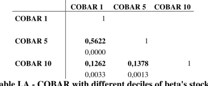
Additionally to the specification proposed by the main paper, COBAR based on the 5th
and 10th decile of the beta of stocks is computed. One can expect Decile 5 COBAR, that is
included as a check against the extreme deciles, to show little correlation with the other
specifications, but as it can be seen in Table I.A it has a correlation of 0,5622 with Decile 1
COBAR. On the other hand, Decile 5 COBAR presents a correlation of 0,1378 with the Decile
10 COBAR. The correlation between Decile 1 and Decile 10 is only 0,1262. It can then be
concluded that the results of the abnormal returns of the beta strategy will be different if
COBAR is used based on 1st decile or on 10th decile. In this thesis it was chosen to build the
COBAR measure with the 10th decile because it can be capturing the trend not only of the
long-short strategy but also of the long-only strategy, which, in general, is easier to
13
COBAR 1 COBAR 5 COBAR 10
COBAR 1 1
COBAR 5 0,5622 1
0,0000
COBAR 10 0,1262 0,1378 1
0,0033 0,0013
Table I.A - COBAR with different deciles of beta's stocks
COBAR is then computed using the entire sample and a sample that excludes penny
stocks (stocks priced below $5). As it can be observed in Table I.B, the correlation between
the two specifications is significantly high, 0,9854. For further research, COBAR was
computed using the entire sample since excluding penny stocks is not expected to produce
very different abnormal returns.
COBAR COBAR np
COBAR 1
COBAR np 0,9854 1
0,0000
Table I.B - COBAR without penny stocks (<5$)
COBAR is computed based on the 3-factor and on the 6-factor model. As it can be
observed in Table I.C, the two specifications are highly correlated (0,9907). It can be
concluded that adjusting the measure for the 6-factor model will result in similar outcomes as
compared to the usage of the 3-factor model. The main paper approach will be followed and
the COBAR based on 3-factor model will be used.
COBAR COBAR 6f
COBAR 1
COBAR 6f 0,9907 1
0,0000
Table I.C - COBAR with 3 factors of Fama & French and with 6 factors of Fama &
French
Based on the previous conclusions, the following research will be based on the
14 seen in Table II.A, COBAR shows variations along time. COBAR is a measure for the level of
arbitrage activity, so there are clearly periods in which arbitrage activity is higher, reaching a
maximum of 0,665 and others when it is lower, going until -0,035.
Variable N Mean Std. Dev Min Max
COBAR 539 0,202 0,202 -0,035 0,665
Inflation 539 0,043 0,020 0,016 0,092
Sentiment 537 0,000 0,009 -0,023 0,031
Ted Spread 359 0,058 0,045 0,012 0,396
Table II.A – Summary Statistics
In addition, the thesis includes control variables that literature has shown to be
associated with the variation of expected abnormal returns of the beta strategy throughout
time. Based on the Correlation Matrix shown in Table II.B, it is possible to verify that the
arbitrage measure has a negative correlation with Inflation and with Ted Spread, and almost
no correlation with Market Sentiment.
COBAR Inflation Sentiment Ted Spread
COBAR 1
Inflation -0,584 1
Sentiment 0,058 -0,082 1
Ted Spread -0,354 0,462 -0,014 1
Table II.B – Correlation Matrix
In Graph I it is observable that the sample’s level of COBAR is much higher in the
latest years than in the beginning. It is also possible to see that the measure presents cycles,
15
Graph I - Historical data of COBAR from 1970 until 2015
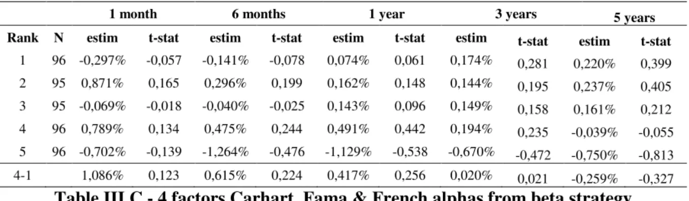
4.2 Dynamic Returns of Beta Strategy
After building COBAR the beta strategy is computed, which consists of going long on
the bottom deciles of stocks and short on the highest decile of stocks. The abnormal returns of
the strategy after 1 month, 6 months, 1 year, 3 years, and 5 years of the beta-arbitrage trade
can be observed in Table III.C (in Tables III of the Appendixes, analysis with investment
horizons of 3 months, 2 years and 4 years can be found). The abnormal returns are the alphas
of the regressions using the 4-factors model of Carhart, Fama & French. For comparison and
consistency of results, the abnormal returns are computed using as well the CAPM, the
3-factors, the 5-3-factors, and the 6-factors model, which can be found in Table III.A, Table III.B,
Table III.D and Table III.E of the Appendixes.
-0,1 0 0,1 0,2 0,3 0,4 0,5 0,6 0,7 0,8
1971 1972 1973 1974 1975 1976 1978 1979 1980 1981 1982 1983 1985 1986 1987 1988 1989 1990 1992 1993 1994 1995 1996 1997 1999 2000 2001 2002 2003 2004 2006 2007 2008 2009 2010 2011 2013 2014 2015
Historical evolution of COBAR
16
1 month 6 months 1 year 3 years 5 years
Rank N estim t-stat estim t-stat estim t-stat estim t-stat estim t-stat
1 96 -0,297% -0,057 -0,141% -0,078 0,074% 0,061 0,174% 0,281 0,220% 0,399 2 95 0,871% 0,165 0,296% 0,199 0,162% 0,148 0,144% 0,195 0,237% 0,405
3 95 -0,069% -0,018 -0,040% -0,025 0,143% 0,096 0,149% 0,158 0,161% 0,212 4 96 0,789% 0,134 0,475% 0,244 0,491% 0,442 0,194% 0,235 -0,039% -0,055
5 96 -0,702% -0,139 -1,264% -0,476 -1,129% -0,538 -0,670% -0,472 -0,750% -0,813
4-1 1,086% 0,123 0,615% 0,224 0,417% 0,256 0,020% 0,021 -0,259% -0,327
Table III.C - 4 factors Carhart, Fama & French alphas from beta strategy
The samples of abnormal returns of the different investment horizons (1 month, 6
months, 1 year, 3 years and 5 years) are ranked in values of COBAR with the lowest values
identified as periods with lowest beta arbitrage activity, and the highest values identified as
periods with highest beta arbitrage activity. Table III.C shows that for the lower values of
COBAR, the average of the abnormal returns takes longer to materialize, being negative in the
1st (-0,297%) and 6th (-0,141%) months and become positive in the 1st year (0,074%), growing
until the 5th years (0,220%). This pattern is similar to the one presented in the main paper.
Yet, for the higher values of COBAR, the pattern is very different from the one presented in
that paper. In fact, it can be observed that for a large volume of beta arbitrage in the market,
the abnormal returns are always negative, independently of the time period considered. In the
1st month, the average abnormal return is -0,702%, in the 6th month it is -1,2264%, in the 1st
year it is -0,670% and in the 5th year it is -0,750%. What can be comparable to the results of
the main paper is the rank 4 sample of COBAR: the abnormal returns are positive in the short
run (1st month = 0,789%; 1st year = 0,491%) and become negative if the investor keeps
collecting returns from the strategy until the 5th year (-0,039%). These patterns can be easier
understood in Graph II.
The main study argues that the abnormal 4-factor returns of the beta strategy need
more time to materialize in periods with lower arbitrage volume (lower ranks), being only
positive in the 2nd and 3rd years (in this thesis, the analysis is extended until the 5th year
17 high in the 6th month. The authors conclude that these quicker and stronger abnormal returns
face a reversal in the long run (3rd year).
The divergent results presented in this thesis can be explained in accordance with the
ones presented in the main paper. In fact, it could be observed in Graph I that values of
COBAR are much higher in the latest years of the sample, namely from 2010 until 2015. The
main papers’ sample covers the period from 1965 until 2010, while this thesis covers the one
from 1970 until 2015. As a consequence the values of high COBAR must coincide with the
sample period of 2010-2015, causing the pattern to be somewhat different. By analyzing
Graph II, it can be concluded that when COBAR is very high, which translates into a very
high volume of beta-arbitrage, investors cannot realize positive returns at least until the 5
years investment horizon. This can be explained by investors causing disruptions in prices
which lead them to levels that don’t coincide with their true value. After the investors
pursuing the strategy and the stocks’ price suffer a big jump, they will quickly return to its
“equilibrium” price causing investors not to reach the expected profits from the strategy.
Additionally, it can be observed in Graph II that the relationship between COBAR and
abnormal returns is similar to the one shown in the main paper for the ranks 1 and 4. In
periods of low COBAR, there is a delay in the abnormal returns collected by investors.
However, once more beta arbitrage investors participate in the market, these abnormal returns
can be received in shorter periods, being reversed in the long run. This behavior is consistent
with a price overshoot due to the signal transmitted to investors, who want to participate in
the market in order to gain from the strategy. Since too many investors will want to take
advantage of the strategy, the stock price will go above its equilibrium price (from the channel
of demand, and not due to its fundamental value). Once the period with the high demand for
the stocks passes, the price of stocks will start decreasing, causing investors to have negative
18
Graph II - Abnormal Returns of 4 Factors Carhart, Fama & French split by ranks of
COBAR
In order to confirm the patterns shown above, a regression of the abnormal 4-factor
returns on COBAR and other control variables that were shown to predict beta-arbitrage
returns is included in Table V.A. Here, the Value Spread is included, which was computed
following the approach of Cohen, Polk, & Vuolteenaho (2005) because it was argued by the
authors that the value spread can have some impact on the returns of the beta strategy. The
market volatility of the previous 12 months of each portfolio formation date is also included.
The regressions do not only take into account the ordinal value of COBAR but also the
cardinal values. Therefore, they seem to present the predictive power of the variables that
literature demonstrated to impact beta-strategy returns in the presence of the innovative
variable. In Table V.B of the Appendixes, the regressions are computed by using the
abnormal returns with the 6-factor models as a dependent variable with the objective to ensure
consistency in the results presented.
Regressions (1) to (3) forecast the time series variations in the abnormal 4-factor
beta-arbitrage returns in the 6 months investment horizon following the portfolio formation.
Regression (1) confirms that COBAR contributes negatively significantly (-0,0586) for the -0,015
-0,01 -0,005 0 0,005 0,01
1m 3m 6m 1y 2y 3y 4y 5y
Abnormal Returns of 4 factors Carhart, Fama & French splited by ranks of COBAR
19 abnormal returns of the strategy. Regression (2) includes control variables that have data
available for the sample under investigation. Regression (3) includes all variables. As it can
be observed, only COBAR has statistical significance in forecasting the abnormal returns, and
the sign of the coefficient remains negative in all regressions computed.
Regressions (4) to (6) forecast the abnormal 4-factor beta-arbitrage returns in the 3
years investment horizon. It can also be shown that the coefficient of COBAR remains
significantly negative, yet with lower absolute value than in the previous regressions. The
results can be connected to the conclusions that were drawn in the main paper, in particular
returns of the strategy invert in the long run. In this sample there are periods of very high
COBAR that make the abnormal returns to be always negative (as shown in the previous
section) regardless of the investment horizon, so although the coefficient becomes less
negative, it doesn’t reach the point of inverting. When all control variables are included,
COBAR loses its predictive power and Mkt Vol 12 and the Ted Spread become significant. If
the 6 factors model is considered, COBAR remains significant as well as Sentiment and the
20
6 months 3 years
(1) (2) (3) (4) (5) (6)
COBAR -0,0386 -0,0351 -0,0444 -0,0209 -0,0189** -0,0185
-2,28 -1,87 -1,92 -1,67 -1,24 -1,01
Inflation 0,0742 -0,0811 -0,0266 0,0322
0,77 -0,23 -0,38 0,19
Sentiment 0,0858 0,1728 -0,0421 -0,1334
0,47 0,47 -0,45 -0,79
Value Spread -0,0016 0,0002 -0,0022 -0,0011
-0,43 0,04 -0,80 -0,35
Mkt Vol 12 0,4093 0,2682 -0,2342 -0,4201***
0,81 0,45 -0,84 -1,53
Ted Spread -0,0151 0,0542
-0,25 1,88
Nº Obs 502 502 322 502 502 322
Table IV.A - Forecasting 4 factors Carhart, Fama & French abnormal returns
4.3 Beta Expansion
It could be expected that when the stocks included in the strategy are relatively more
leveraged, from the mechanism described by Modigliani & Miller (1958), the impact on
prices of the positive-feedback trading (signals transmitted to investors to trade stocks) is
larger. In fact, if the price of a security rises because many investors decided to invest in those
securities, and in the particular case when stocks are leveraged, the MM Proposition II
proposes that the price of these stocks will increase even more in comparison to stocks with
lower Debt to Equity ratios (inverse mechanisms in the opposite direction of prices). This
increase/ decrease in prices will affect the beta of these stocks, increasing the intensity of the
signals transmitted to the arbitrageurs and thus, investors can reinforce their strategy with
stocks that are already away from their fundamental prices. This mechanism was tested as
21 In regressions (1) and (2), the dependent variable is the spread in betas of the
value-weighted portfolio of stocks included in the strategy in the formation year after one year of
holding those stocks. The independent variables are COBAR in the portfolio formation year,
Beta Spread of the stocks of the strategy in the portfolio formation year, the average book
leverage quintile of the portfolio computed in each formation period, and an interaction
between Leverage and COBAR. Contrary to the main paper, the results of regressions (1) and
(2) are not statistically significant and therefore become erroneous to draw conclusions.
In regressions (3) and (4), the dependent variable is the fraction of stocks in the
low-beta decile, computed in year t and that remain in the low-low-beta decile in year t+1. It needs to
be noted that there is no overlapping in the two periods of Beta Spread and Fraction as betas
were estimated using 52 weeks stocks data. Regression (3) shows that when COBAR is high,
the fraction of stocks remaining in the low beta decile is statistically significantly higher.
When Leverage and the interaction between COBAR and Leverage are included, the impact of
COBAR is no longer significant and Leverage has a negative statistically significant impact,
though very close to zero.
Beta Spread t+1 Fraction t+1
(1) (2) (3) (4)
Beta Spread t 0,0701** 0,0681**
1,21 1,15
COBAR -0,3885 0,2145 0,0343*** 0,0261
-0,43 0,15 1,44 0,61
Leverage 0,1314 -0,0060***
0,73 -1,54
COBAR*Leverage -0,2182 0,0038
-0,48 0,32
Nº Obs 527 527 527 527
22
5. Conclusion
The thesis studies the relations between arbitrage activity and the abnormal returns of
the beta strategy. Using the novel measure COBAR as a proxy for the level of arbitrage
activity, it was verified that for very high level of arbitrage activity the abnormal returns of
the beta strategy are always negative, independently of the holding period considered by the
investor. This conclusion is not equal to the one shown in the main paper, which is explained
for the extended sample used in this thesis. Additionally, the leverage of stocks as a fact that
can widen the beta spread in the portfolio in periods with high COBAR could not be
concluded. Besides that, it was proved significant that these periods of high COBAR have a
positive relation with the stocks that remain in the low beta decile from one year to the other.
The main weaknesses of this thesis are related to the access to data and the complexity
of methodology. On the one hand, the variable Assets under Management, Institutional
Ownership, and Disagreement were not possible to be computed due to missing public access
to data or computations with a complexity that goes beyond the scope of this thesis. On the
other hand, the methodology could have been done differently which certainly could result in
different results. For example, a one-year ranking period consideration, sample with only
stocks from the NYSE, average formula of returns considered, the number of trading days
static for each year (260), month (22) and week (5). Moreover, the transaction costs of
performing the strategy are not being taken into account, which can also be considered a
limitation of this thesis.
Besides its limitations, this thesis continues the work of Lou, Polk, & Huang (2016)
and can have an impact on how investors, who intend to pursue the beta strategy, decide to
invest. In fact, if they can calculate the values of COBAR and have a historical sample of these
values, they can identify which periods are more likely to result in higher returns (periods
23 (between 1 month and 1 year). These strategies are usually easier to implement by
professional investors such as Asset Managers and Hedge Funds due to the decreased
transactions costs they can be exposed to.
References
Antoniou, C., Doukas, J. A., & Subrahmanyam, A. (2013). Investor Sentiment, and Beta
Pricing. UCLA working paper.
Baker, M., & Wurgler, J. (2007). Investor Sentiment in the Stock Market. Journal of
Economic Perspectives, 21, 129-152.
Baker, M., Bradley, B., & Taliaferro, R. (2013). The Low Risk Anomaly: A Decomposition
into Micro and Macro Effects. Harvard Business School working paper.
Bali, T., Cakici, N., & Whitelaw, R. (2011). Maxing Out: Stocks as Lotteries and the
Cross-Section of Expected Returns. Journal of Financial Economics, 99, 427-446.
Barberis, N., & Huang, M. (2008). Stocks as Lotteries: The Implications of Probability
Weighting for Security Prices. American Economic Review, 98, 2066-2100.
Barberis, N., & Shleifer, A. (2003). Style investing. Journal of Financial Economics, 68,
161-199.
Barberis, N., Shleifer, A., & Wurgler, J. (2005). Comovement. Journal of Financial
Economics, 75, 283-317.
Black, F. (1972). Capital Market Equilibrium with Restricted Borrowing. Journal of Business,
45, 444-454.
Black, F., Jensen, M. C., & Scholes, M. (1972). The Capital Asset Pricing Model: Some
Empirical Tests. Studies in the Theory of Capital Markets, 79-121. (N. Y. Praeger,
Ed.)
Blitz, D., & Vliet, P. V. (2007). The Volatility Effect: Lower Risk Without Lower Return.
24 Blitz, D., Pang, J., & Villet, P. V. (2012). The Volatility Effect in Emerging Markets. Robeco
Asset Management working paper.
Campbell, J. Y., & Vuolteenaho, T. (2004). Inflation Illusion and Stock Prices. National
Bureau of Economic Research working paper.
Carhart, M. M. (1997). On Persistence in Mutual Fund Performance. Journal of Finance, 52,
57-82.
Cohen, R. B., Polk, C., & Vuolteenaho, T. (2005). Money Illusion in the Stock Market: The
Modigliani-Cohn Hypothesis. Quarterly Journal of Economics, 70, 639-668.
Cohen, R. B., Polk, C., & Vuolteenaho, T. (2005). The Value Spread. Journal of Finance, 58,
609-641.
Fama, E. F., & French, K. R. (1992). The Cross-Section of Expected Stock Returns. Journal
of Finance, 47, 427-465.
Fama, E. F., & French, K. R. (1993). Common Risk Factors in the Returns on Stocks and
Bonds. Journal of Financial Economics, 3-56.
Fama, E. F., & French, K. R. (2014). A Five-Factor Asset Pricing Model. Journal of Finance,
116, 1-22.
Frazzini, A., & Pedersen, L. H. (2014). Betting Against Beta. Journal of Financial
Economics, 111, 1-25.
Friedman, M. (1966). The Methodology of Positive Economics. Essays in Positive
Economics, 3-16, 30-43.
Haugen, R., & Heins, A. (1975). Risk and the Rate of Return on Financial Assets: Some Old
Wine in New Bottles. Journal of Financial and Quantitative Analysis, 775-784.
Hayek, F. A. (1945). The Use of Knowledge in Society. The American Economic Review, 35,
519-530.
25 Hugonnier, J., & Prieto, R. (2015). Asset pricing with arbitrage activity. Journal of Financial
Economics, 115, 411-428.
Keynes, J. M. (1936). The General Theory of Employment, Interest, and Money. Macmillan
Cambridge University Press.
Kumar, A. (2009). Who gambles in the stock market? Journal of Finance, 64, 1889-1933.
Lakonishok, J., Shleifer, A., & Vishny, R. W. (1992). The impact of institutional trading on
stock prices. Journal of Economics, 32, 23-43.
Lintner, J. (1965). The Valuation of Risky Assets and the Selection of Risky Investments in
Stock Portfolios and Capital Budgets. Review of Economics and Statistics, 47, 13-37.
Lou, D., & Polk, C. (2014). Comomentum: Inferring Arbitrage Activity from Return
Correlations. London School of Economics working paper.
Lou, D., Polk, C., & Huang, S. (2016). The Booms and Busts of Beta Arbitrage. London
School of Economics working paper.
Miller, E. M. (1977). Risk, Uncertainty, and Divergence of Opinion. Journal of Finance, 32,
1151-1168.
Modigliani, F., & Cohn, R. (1979). Inflation, Rational Valuation, and the Market. Financial
Analysts Journal, 35, 24-44.
Modigliani, F., & Miller, M. H. (1958). The Cost of Capital, Corporation Finance, and the
Theory of Investment. American Economic Review, 48, 655-669.
Sharpe, W. (1964). Capital Asset Price: A Theory of Market Equilibrium under Conditions of
Risk. Journal of Finance, 19, 425-442.
Stein, J. (2009). Sophisticated Investors and Market Efficiency. Journal of Finance.
Stein, J. C. (1987). Informational Externalities and Welfare-reducing Speculation. Journal of