3DArm Inertial Sensor-based 3D Upper Limb Motion Tracking and Trajectories Reconstruction

motion tracking and trajectories

reconstruction

Ana Cristina Campos Pereira

Supervisor at FEUP: Miguel Velhote Correia, PhD Supervisor at FhP-AICOS: Vânia Guimarães, MSc

Integrated Master in Bioengineering

Inertial sensor-based 3D upper limb motion tracking and

trajectories reconstruction

Ana Cristina Campos Pereira

Dissertation submitted to Faculdade de Engenharia da Universidade do Porto to obtain the degree of

Master in Bioengineering

Upper limb motion tracking plays a major role in several applications such as movement evalua-tion of workers, gaming, human-machine interacevalua-tion and medical rehabilitaevalua-tion. There are many systems to perform upper limb tracking - they can be non-visual (inertial), visual (with markers or marker-free) or robot-aided. Despite this variety of tracking systems, they have limitations and some of these systems also consist of specifically designed sensors and tend to be designed for a specific goal, making them unsuitable for acting in all the applications mentioned above. This way, the need for a global upper limb motion tracking solution arises.

For that purpose, the 3DArm - Upper Limb Inertial Tracking System was developed. Based on literature review, this system was built in order to track the upper limb for various applications. In order to do that, two inertial sensors were placed on the upper and lower arms and the upper limb was modeled so that the joints and movements could be described in a global body reference frame. Then, data from inertial sensors were combined through an Extended Kalman Filter sensor fusion method with biomechanical constraints, in order to obtain orientation. The sensors were aligned with each other and with the global body reference frame so that the upper limb position could be described in the global body frame. After finding sensor orientation relative to the global body frame, the upper limb kinematic model was used to reconstruct upper limb motion.

To evaluate the system, 3DArm was compared to Kinect and, in spite of the small deviation between them - a maximum mean error of 10,60 centimeters and 16,33 centimeters for the elbow and wrist joints, respectively - the experimental results demonstrated that the proposed tracking system had an acceptable performance, in different movements. Therefore, 3DArm can be consid-ered a viable tracking system with the advantages of being portable, without occlusion problems, small-sized, unobtrusive, low-cost and lightweight.

Moreover, it was difficult to guarantee that the two sensors were aligned with each other. To overcome this problem, a sensor-to-body frame transformation, without the need of aligning the sensors with each other and with the global body reference frame, was developed. With a calibration movement, each axis of the global body reference frame was defined. The results of the sensor-to-body frame transformation showed that the calculated elbow and wrist positions resulted in errors in the same order as the ones reported when sensors were manually aligned on each arm segment.

Although results were promising, further development of this project is required to potentially improve upper limb motion tracking.

Keywords: Upper Limb. Inertial Tracking. Sensor Fusion. Orientation Estimation. Quater-nions. Extended Kalman Filter. Trajectory Reconstruction.

O tracking do movimento do membro superior tem uma grande importância em várias aplicações, como a avaliação do movimento de trabalhadores, jogos, interacções homem-máquina e reabili-tação médica. Existem muitos sistemas de tracking do membro superior; estes podem ser não-visuais (inerciais), não-visuais (com ou sem marcadores) ou assistidos por robôs. Apesar desta var-iedade de sistemas de tracking, estes têm limitações e alguns utilizam sensores específicos conce-bidos para objectivos muito restritos, tornando-os inadequados para todas as aplicações. Assim, surge a necessidade de uma solução global de tracking do movimento do membro superior.

Com isso em mente, foi desenvolvido o 3DArm - Upper Limb Inertial Tracking System. Baseado numa revisão da literatura, este sistema foi construído de forma a fazer o tracking do membro superior para qualquer aplicação. Para isso, foram colocados dois sensores inerciais nos segmentos superior e inferior e o membro superior foi modelado de forma a que as articulações e movimentos pudessem ser descritos num sistema corporal global. De seguida, os dados dos sensores inerciais foram combinados através de um método de sensor fusion Extended Kalman Filtercom restricções biomecânicas, para obter a sua orientação. Os sensores foram alinhados um com o outro e com o sistema corporal global, de forma a que a posição do membro superior pudesse ser descrita nesse mesmo sistema. Após calculada a orientação relativamente ao sistema corporal global, o modelo cinemático do membro superior foi utilizado para fazer a reconstrução do movimento.

Para avaliar o sistema, o 3DArm foi comparado com o Kinect e, apesar do pequeno desvio entre eles - um erro médio máximo de 10,60 centímetros e de 16,33 centímetros para o cotovelo e pulso respectivamente - os resultados experimentais demonstraram que o sistema de tracking proposto tinha uma prestação aceitável, com diferentes movimentos. Desta forma, o 3DArm pode ser considerado um sistema de tracking viável com as vantagens de ser portátil, sem problemas de oclusão, pequeno, não-obtrusivo, barato e leve.

Foi difícil garantir que os dois sensores estavam efectivamente alinhados um com o outro. Para ultrapassar este problema, foi desenvolvida uma transformação de sistema sensor-para-corpo que não requer o alinhamento dos sensores consigo próprios nem com o sistema corporal global. Com um movimento de calibração, cada eixo do sistema corporal global foi definido. Os resultados da transformação de sistema sensor-para-corpo mostraram que as posições do cotovelo e pulso calculadas originaram erros da mesma ordem que os erros quando os sensores eram manualmente alinhados em cada segmento do braço.

Apesar de os resultados serem promissores, é necessário mais desenvolvimento deste projecto de forma a potencialmente melhorar o tracking do membro superior.

Keywords: Membro Superior. Tracking Inercial. Sensor Fusion. Estimação da Orientação. Quaterniões. Extended Kalman Filter. Reconstrução de Trajectórias.

Miguel Velhote Correia, pela orientação na minha dissertação, pelo seu apoio e experiência. À Fraunhofer Portugal AICOS, pelas instalações e equipamento que tornarem possível a realização do meu trabalho. À minha orientadora Vânia Guimarães, pelo apoio, conhecimento, sugestões, motivação e esforço para que tudo corresse sempre da melhor maneira, pela disponiblidade para todos os assuntos, desde os mais simples aos mais complexos.

Um grande obrigada a todos os meus amigos que marcaram estes cinco anos e os tornaram no mínimo inesquecíveis.

O obrigada ao Miguel, por tudo e mais alguma coisa. Pelos conselhos, avisos, pela grande força e motivação incondicionais. Por ter-me feito acreditar em mim e no meu trabalho. Por ser tão chato e tão preocupado e por estar motivado a aprender as lides da casa.

Um último obrigada, mas não menos importante, aos meus pais, irmão e infinita família. Aos meus pais por terem permitido tudo isto ser possível e apoiarem-me em todos os momentos. Ao João, por termos crescido juntos e continuarmos a crescer. À família toda, aos grandes Santas, aos meus avôs que estão lá a olhar por mim, e às minhas avós, as mulheres mais fortes que conheço.

Ana Pereira

List of Tables xiii

List of Abbreviations xv

1 Introduction 1

1.1 Problem Identification . . . 2

1.2 Motivation and Objectives . . . 2

1.3 Dissertation Structure . . . 3

2 Background and Literature Review 5 2.1 Modeling of the Upper Limb Movement . . . 5

2.1.1 Upper Limb Joints and Movements . . . 5

2.1.2 Kinematic Model . . . 9

2.2 Inertial Tracking . . . 12

2.2.1 Inertial Measurement Unit . . . 12

2.2.2 Sensor Fusion for Orientation Estimation . . . 13

2.2.3 Attitude Representation . . . 19

2.3 Position and Trajectory Reconstruction . . . 22

2.4 Sensor-to-Body Frame . . . 25

3 3DArm - Upper Limb Inertial Tracking System 27 3.1 3DArm Overview . . . 27

3.2 Data Acquisition . . . 28

3.2.1 Inertial Sensors . . . 28

3.2.2 Kinematic Model and Global Body Reference Frame . . . 29

3.3 Signal Pre-Processing . . . 30

3.3.1 Low-Pass Filter . . . 30

3.3.2 Data Normalization . . . 30

3.4 Sensor to Global Body Reference Frame . . . 31

3.5 Orientation Estimation . . . 32

3.5.1 TRIAD Algorithm . . . 32

3.5.2 Extended Kalman Filter . . . 34

3.6 Position and Trajectory Reconstruction . . . 38

3.7 3DArm Evaluation . . . 39

3.7.1 Experimental Work . . . 40

3.7.2 Results and Discussion . . . 43

3.8 Proof of Concept . . . 52

4 Sensor-to-Body Frame 55

4.1 Preliminary Evaluation . . . 55

4.1.1 Experimental Work . . . 56

4.1.2 Results and Discussion . . . 57

4.2 Data Acquisition . . . 61

4.2.1 Kinematic Model and Global Body Frame . . . 61

4.2.2 Acquisition Protocol . . . 61

4.3 Theoretical Formulations . . . 63

4.3.1 Definition of posture vectorss_rU t andsrLt . . . 63

4.3.2 Global Body Reference Frame definition . . . 64

4.3.3 Definition ofbrU₀,brL₀,bqU_t andbqL_t . . . 64

4.4 Results and Discussion . . . 65

4.4.1 Definition of t1and t2 . . . 65

4.4.2 Definition of Angular and Linear Velocities . . . 68

4.4.3 Position and Trajectory Reconstruction . . . 70

5 Conclusions and Future Work 75 5.1 Future Work . . . 76

References 79

A Rotation Matrix ⇒ Unit Quaternion 83

forearm and hand) of the upper limb [14]. . . 6

2.2 Upper Limb Joints [14]. . . 7

2.3 Simplified movement system in the arm [16]. . . 8

2.4 Simplified movement system in the forearm [16]. . . 9

2.5 The plane and axis. Movement takes places in a plane about an axis perpendicular to the plane [15]. . . 10

2.6 Upper limb model [18]. The right arm is depicted viewed from the back, where L1 and L2represent the upper and lower segments’ length, respectively. . . 11

2.7 Fusion of the different sensor readings in order to get the best attitude estimation [29]. 14 2.8 A complete description of the operation of the EKF [34]. . . 18

2.9 Earth Reference Frame [29]. . . 19

2.10 The orientation of frame B is achieved by a rotation, from alignment with frame A, of angle θ around the axisA_{r [38]. . . . . 21}

2.11 Inertial tracking relative to the global frame [18]. . . 23

3.1 3DArm flowchart. . . 28

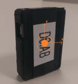
3.2 Pandlet developed at FhP-AICOS. Sensor’s local reference system is presented in orange. . . 29

3.3 Position and orientation of sensors. GB Reference Frame is red and sensors’ local reference frame are black. Origin is green. . . 30

3.4 Block diagram of EKF design. . . 33

3.5 Block diagram of the process model for orientation quaternion. q is the orientation quaternion, ˙qis the quaternion derivative, ˆqis the estimated quaternion and w is the angular velocity. . . 35

3.6 Extended Kalman Filter implementation diagram. . . 38

3.7 Skeletal tracking using a skeletal representation of various body parts. Each part or joint is represent by its correspondent tracking point. . . 40

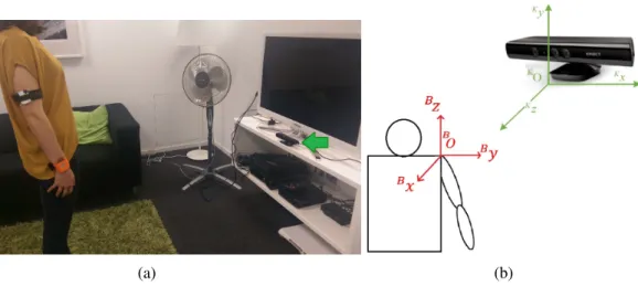
3.8 User and Kinect. (a) Experimental environment setup (Kinect system marked with green arrow). (b) The GB reference frame OBxByBz(seen from the back) and the Kinect frame OKxKyKz. . . 41

3.9 Test 1 - shoulder abduction/adduction. . . 42

3.10 Test 2 - shoulder flexion/extension. . . 43

3.11 Test 3 - shoulder extension, rotation to the coronal side and shoulder adduction. . 43

3.12 Angle related to the abduction/adduction movement of the elbow joint during Test 1, 2 and 3. Blue line represents the result from the EKF sensor data fusion with biomechanical constraint, whereas green line indicates the result from the CF sen-sor data fusion without biomechanical constraint. . . 45

3.13 Test 1 - Elbow and wirst positions (centimeters) along time (seconds). The blue line represents the 3DArm results and the red line represents the Kinect results. A lag between the 3DArm and the Kinect signal and an amplitude difference are present. . . 48 3.14 Test 1 - Elbow and wrist positions along time (a), in the xz-plane (b) and in the

yz-plane (c). In (a), the blue line represents the 3DArm results and the red line represents the Kinect results. In (b) and (c) the red is for the elbow and green for the wrist; the line represents the 3DArm results and the dots the Kinect results. . 49 3.15 Test 2 - Elbow and wrist positions along time (a), in the xz-plane (b) and in the

yz-plane (c). In (a), the blue line represents the 3DArm results and the red line represents the Kinect results. In (b) and (c) the red is for the elbow and green for the wrist; the line represents the 3DArm results and the dots the Kinect results. . 50 3.16 Test 3 - Elbow and wrist positions along time (a), in the xz-plane (b), in the

yz-plane (c) and in the xy-yz-plane (d). In (a), the blue line represents the 3DArm results and the red line represents the Kinect results. In (b), (c) and (d) the red is for the elbow and green for the wrist; the line represents the 3DArm results and the dots the Kinect results. . . 51 3.17 Kinect occlusion problem in Test 2 (shoulder flexion/extension). . . 52 3.18 Free movement test: (a) and (c) are photos of the subject performing a free

move-ment, (b) and (d) are the real-time results of the visualization tool reproducing movements (a) and (b). Letters s, e and w represent the shoulder, elbow and wrist joint, respectively. . . 53 4.1 Wodden Armplaced on the desk. . . 56 4.2 Movement sequence for Test 1 (a) and for Test 2 (b). The black reference system

corresponds to the sensor reference frame and the green reference system to the global reference system. L represents the length of the segment, that is, from the origin O to the place where the sensor was mounted, and is the same for Test 1 and 2. 57 4.3 Test 1 results. Positions for each axis are represented in (a) and absolute errors are

represented in (b). In (b) the time it is not continuous, instead it is represented by a point that corresponds to the stage where the sensor was in that time. . . 59 4.4 Test 2 results. Positions for each axis is represented in (a) and absolute errors are

presented in (b). In (b) the time it is not continuous, instead it is represented by a point that corresponds to the stage where the sensor was in that time. . . 60 4.5 Sensor’s attachment in Configuration 1 (a) and 2 (b). . . 62 4.6 Calibration movement sequence: (a) Down1 refers to the initial phase when the

arm is stationary, from time 0 to time t1, (b) Swing refers to the pahse when the

arm is swinging, from time t1to t2, and (c) Down2corresponds to the phase when

the arm returns to the initial position. . . 62 4.7 Scheme to determines_g. b_xb_yb_{zrepresent the GB reference frame,}b_{gis the}

gravi-tational acceleration vector,sq2,3is the mean orientation quaternion from seconds

2 to 3, which represent the rotation to the sensor initial reference frame andsgis the vectorb_{gdefined in the sensor’ reference frame. . . . 66}

4.8 Scheme to determine EgU_t . ExEyEz represent the earth reference frame, sgis the vectorbgdefined in the sensor’ reference frame andsqt is the sensor orientation

relative to the earth reference frame. . . 66 4.9 Movement phases segmentation with t1and t2represented as dots. . . 67

4.10 Slope of Down1 and Down2phases within a 0.4 seconds (20 points) window for

4.14 Upper and Lower Linear Velocity Magnitude. . . 69 4.15 Configuration 1 - Positions trajectories in x,y and z axes, for elbow and wrist

joints. Positions are represented in cm and time in seconds. . . 73 4.16 Configuration 1 - 3D trajectories (cm) for elbow and wrist joints. . . 73 4.17 Configuration 2 - Positions’ trajectories in x,y and z axes, for elbow and wrist

joints. Positions are represented in cm and time in seconds. . . 74 4.18 Configuration 2 - 3D trajectories (cm) for elbow and wrist joints. . . 74

2.2 EKF time update equations. . . 18

2.3 EKF measurement update equations. . . 18

2.4 Overview of upper limb motion tracking related work. . . 24

3.1 Segment lengths of individual subjects in the experiments (units:cm). . . 42

3.2 Statistical results of the tests performed for elbow and wrist joints, where Std refers to standard deviation and Max to the maximum. All parameters are represented in centimeters (cm). . . 48

4.1 Expected position for each axis in the 4 Stages. Expected positions are represented in centimeters (cm). . . 58

4.2 Upper and Lower lengths real value l, estimation lest and absolute error e, in cen-timeters (cm). . . 70

4.3 Maximum error (in centimeters) for the elbow and wrist positions for each axis in Configurations 1 and 2. . . 72

DOF Degree of Freedom EKF Extended Kalman Filter

FEUP Faculdade de Engenharia da Universidade do Porto

FhP-AICOS Fraunhofer Portugal Research Center for Assistive Information and Com-munication Solutions

GB Global Body

IMU Inertial Measurement Unit ISP Integrated Sensor Pack

KF Kalman Filter

MMSE Minimum Mean Square Error VR Virtual Reality

Upper limb motion tracking has become an extensive research topic in the human motion tracking studies. This is due to its broad range of applications, including movement evaluation of workers, gaming, human machine interaction and medical rehabilitation [1].

Movement evaluation of workers takes place in the factories and it is most needed for work-ers who execute repetitive tasks during their working day. Many industrial work tasks involve extensive arm and hand movements (e.g. short-cyclic assembly and packaging tasks), which are associated with an increased prevalence of musculoskeletal disorders on the neck, shoulders, arms and hands [2]. Thus, an upper limb tracking system can evaluate the worker’s movements and ob-tain several metrics, such as movement amplitude, in order to understand the prevalence of these disorders [3].

Moreover, a new generation of video game consoles enables video gamers to employ active body movements as interaction mode. To achieve a movement-based interaction, the interfaces have to analyze the movement patterns of their users in order to identify them. This is not a trivial task as the human body, in particular the upper limb, is complex and has a large number of degrees of freedom [4]. Tracking the upper limb is one of the main objectives of these video consoles, which is achieved through different techniques, like video and inertial tracking.

Besides this, the study of automatic and natural modes of interaction between humans and machines is an important field of research. For this purpose, it is clearly important not only to locate potential users but also to obtain information about their body posture and arm configu-rations. This task can be complicated due to the high dimensionality of the upper-body and the often unpredictable motion of the arms, so a tracking system is necessary to continuously monitor the upper limb motion [5]. One application of human machine interface is the use of robotics in rehabilitation therapies, since robots are certainly well suited to precisely perform repetitive and mechanically power consuming rehabilitation tasks [6].

Furthermore, major disabilities require extensive rehabilitation programmes in order to treat disabled individuals and prepare them for independent living. The intense repetitions of coordi-nated motor activities during rehabilitation constitute a significant burden for the therapists assist-ing patients. In addition, and due to economical reasons, the duration of primary rehabilitation is

becoming increasingly shorter, since rehabilitation in a hospital-based environment is very expen-sive to the National Health Service and health insurers due to specialists, therapy staffs and the time required. To address this problem, trajectories during rehabilitation have to be quantified and the need for a motion tracking system emerges to allow a rehabilitation process at home. Data on the progress of the patient undertaking home-based rehabilitation could be then passed onto therapists or experts remotely for evaluation. The patients could then adjust their exercises based on the feedback from the therapists or expert systems [7, 8]. Additionally, new rehabilitation tools based on Virtual Reality (VR) and serious games are being developed and have recently gained significant interest in the physical therapy area. These tools also rely on an upper limb tracking system [9].

1.1

Problem Identification

There are many methods and systems to perform upper limb tracking; they can be non-visual (inertial), visual (with markers or marker-free) or robot-aided. Despite this variety of tracking systems, they have some limitations. In summary, an inertial system suffers from drift, a visual system is space-limited, which means that the tracking only occurs within the space where the camera is, and the robot-aided system cannot allow a subject to freely move his/her arm [10]. Another challenge is cost, since people tend to build complicated tracking systems in order to satisfy multiple purposes. These require expensive components on designed systems. Some of these systems also consist of specifically designed sensors, which limit the further development and broad application of the designed systems [7].

The problem identified is the non-existence of an unique portable low-cost system that can be worn in a non-intrusive way by people, allowing a real time upper limb tracking. This happens because the existing systems are focused on a single application, making it difficult for its re-utilization in other contexts.

This way, the problem relies on the need for an upper limb tracking system that can be used by all people in several different contexts, like the applications mentioned above. The system needs to be low-cost and wearable in different environments, allowing a real time tracking.

1.2

Motivation and Objectives

Movement can be measured using a wide variety of techniques and sensors. Several success-ful examples have existed in literature for the application of inertial sensor based systems in the measurements of upper limb movements [11].

Considering the problem mentioned above and the drawbacks of the current tracking tech-niques, an inertial low-cost tracking system should be the solution. Wearable inertial sensors have the advantages of being small-sized, unobtrusive, low-cost, lightweight and self-contained. De-spite the drift problem, once it is corrected, inertial sensors are well suited for recording long-term

movement evaluation of workers, gaming, human machine interaction and medical rehabilitation. This is possible because an inertial system can undergo a process of sensor-to-body frame trans-formation, enabling every person to place the sensors on the arm in a correct way. With an inertial tracking system, it is possible to obtain the upper limb movement and its trajectories, which can be evaluated in real time, enabling the extraction of distinct characteristics (for instance, the move-ment amplitude, the angle between segmove-ments, the movemove-ment velocity, etc.) each one more suitable for distinct applications.

In the movement evaluation of workers, an inertial system would be useful to track the move-ments during the different tasks, since it is a portable system that can follow all the worker’s movements. In gaming, an inertial tracking system overcomes the problem of the user being lim-ited to a certain space in front of the console (like in the Xbox) or having to hold a remote control (like in Nitendo Wii). For a human-machine interaction, an inertial system provides a real-time tracking, allowing for a real time interaction. In rehabilitation, a system like this will provide a home-based rehabilitation, allowing the patient to perform upper limb exercises at home and, at the same time, to be followed by the therapists without the need to go to the medical facilities.

As it can be seen, the development of an inertial motion tracking system can be useful for a variety of applications and not specifically or exclusively for any of them. The tracking system could be used in every situation and can accompany the person’s upper limb movement during the day [12].

Therefore, the main objective of this dissertation is to develop a wearable inertial tracking system to estimate orientation and find the motion trajectories of the humam upper limb. The motion trajectories will be estimated by combining sensor fusion and orientation tracking with biomechanical constraints of the upper limb that will take into account the relationships between each arm segment and the human motion limitations. To avoid the burden of manually aligning the sensors to each other and with the mounted arm segment, an automatic method to discover the alignment of the sensors relative to the arm segments will be studied.

1.3

Dissertation Structure

This dissertation is organized in chapters, each one covering a specific topic, and these are subdi-vided in sections that focus on specific subjects of the said topic.

In Chapter 1 – Introduction, the main purpose is making a first approach of the context and objectives that will be fulfilled in this dissertation and also describing its structure.

In Chapter 2 – Background and Literature Review, the objective is to present an extended overview on upper limb motion tracking and trajectory reconstruction is made. Firstly, there is a description of the modeling of the upper limb movement, based on the joints and range of motion and the kinematic model itself. Secondly, there is a description of inertial measurement unit sensor

fusion, based on the sensors and the orientation representation. Lastly, there is also a strong focus on how inertial upper limb tracking and sensor-to-body processes have been applied in research studies by several authors.

In Chapter 3 – 3DArm - Upper Limb Inertial Tracking System, the work developed in order to obtain an upper limb inertial tracking system will be described. There is a description of the methods implemented and how the system was evaluated, presenting its results and introducing future improvements.

In Chapter 4 – Sensor-to-Body Frame, the objective is to develop a sensor-to-body frame process in order to avoid the burden of manually aligning sensors. Here, the methodology imple-mented is described and the results are discussed also introducing future improvements.

In Chapter 5 – Conclusions and Future Work, a description of what was achieved in this dissertation is shown and future developments are referenced.

This Chapter provides a review of the fundamental topics regarding the upper limb motion tracking and its trajectories reconstruction. Firstly, the modeling of the upper limb is described considering its anatomy and representation in a coordinate frame. Then, inertial tracking is presented as an efficient option to measure upper limb movements and positions. Inertial sensors are described, sensor fusion for orientation estimation is explained based on these sensors, and the methods to represent the orientation output from sensor fusion are presented. With the orientation of each arm segment and with the kinematic model considered before, the upper limb trajectories can be reconstructed. In this part, a review of the work developed in this area is described. Lastly, a sensor-to-body frame process is presented in order to avoid the burden of manually aligning the sensors with each arm segment.

2.1

Modeling of the Upper Limb Movement

Compared to lower limb activity monitoring, the upper limb is more difficult due to a number of complications. Firstly, the higher number of degrees of freedom (DOF) of the upper limb joints means that different people can exhibit entirely different motions for the same activity, and within-subject motions may vary for the same activity. Secondly, the activity may be performed differ-ently depending on physical conditions and surroundings. Lastly, there are no strong, identifiable signatures that distinguish upper body motions. Therefore, few research has been published on activity classification in the domain of upper limb motion, since it is difficult to classify a healthy or unhealthy movement, except those aimed at classifying a strictly defined activity set [13].

The main purpose of modeling the upper limb movement is to define an upper limb model and a reference frame where the positions, and consequently the trajectories of the upper limb movement, will be described.

2.1.1 Upper Limb Joints and Movements

The upper limb skeletal system is divided in four main structures: pectoral girdle, arm, forearm and hand, depicted in Figure 2.1 [14]. Since the first three structures are the ones involved in the

movement of the arm and forearm, those are the most relevant for upper limb motion tracking, which will be developed in the dissertation. The hand is the most distal part of the upper limb and its movement does not influence upper limb motion tracking.

In order to perform the tracking of its movement, it is important to understand which move-ments the upper limb can execute and which joints are involved in those movemove-ments.

Figure 2.1: Representation and bone configuration of the four structures (pectoral girdle, arm, forearm and hand) of the upper limb [14].

2.1.1.1 Joints

Muscles pull on bones to make them move, but movement would not be possible without the joints between the bones. A joint is a place where two or more bones come together. The joints are commonly named according to the bones or portions of bones that join together [14]. Regarding the upper limb, there are two fundamental joints:

• Shoulder Joint - the shoulder joint, or glenohumeral joint, is a ball-and-socket joint (Fig-ures 2.2a and 2.2b) in the arm segment. The rounded head of the humerus articulates with the shallow glenoid cavity of the scapula.

• Elbow Joint - the elbow joint is a compound hinge joint (Figures 2.2c and 2.2d) consisting of the humeroulnar joint, between the humerus and ulna, and the humeroradial joint, between the humerus and radius. The elbow joint is surrounded by a joint capsule.

(a) Ball and socket (b) Glenohumeral

(c) Hinge (d) Cubital

Figure 2.2: Upper Limb Joints [14].

2.1.1.2 Movements

A joint’s structure relates to the movements that occur at that joint. Different basic movements occur in different combinations in the body joints. Regarding the upper limb, two types of move-ments can be considered:

• Angular Movements - in angular movements, one part of a linear structure, such as the trunk or a limb, bends relatively to another part of the structure, thereby changing the angle between the two parts. The most common angular movements are flexion and extension and abduction and adduction. Flexion is a bending movement in which the relative angle of the joint between two adjacent segments decreases. Extension is a straightening movement in which the relative angle of the joint between two adjacent segments increases as the joint returns to the zero or reference position. Abduction is a movement away from the midline of the body or the segment. Lastly, adduction is the return movement of the segment back toward the midline of the body or segment [14, 15].

• Circular Movements - Circular movements involve rotating a structure around an axis or moving the structure in an arc. The most common circular movements are supination and pronation, rotation and circumduction. Supination and pronation refer to the unique rotation of the forearm. Supination is the movement of the forearm in which the palm rotates to face forward from the fundamental starting position. Pronation is the movement in which the palms face backwards. Rotation is the turning of a structure around its long axis, as in rotating the head, the humerus, or the entire body. Medial rotation of the humerus with the forearm flexed brings the hand toward the body. Lateral rotation of the humerus moves the hand away from the body. Lastly, circumduction is a combination of flexion, extension, abduction, and adduction [14, 15].

The range of motion describes the amount of mobility that can be demonstrated in a certain joint [14]. As mentioned before, the most important joints when studying the movement of the

(a) Elevation and depression (b) Flexion and extension (c) Medial and lateral rotation

Figure 2.3: Simplified movement system in the arm [16].

upper limb are the shoulder joint and the elbow joint, since they determine the range of motion of the arm and forearm. The following values of range of motion in each type of movement are relative to the anatomical position (the position where it is not exerted any force to move it). Those values were estimated from average body measurements [16], on which the shoulder-elbow length was estimated at 36,33 centimeters and the elbow-hand length was estimated at 47,49 centimeters.

Shoulder Joint

The shoulder or glenohumeral joint can perform several types of movements, such as flexion, extension, abduction, adduction, rotation and circumduction [14]. The glenohumeral joint is re-sponsible for the movement of the arm. The arm is able to elevate itself up to 180◦ and suffer a depression of 20◦(in this case, elevation and depression corresponds to adduction and abduction, respectively), while its flexion movement may reach 180◦and its extension may reach 60◦. The arm is also able to perform rotation movements of 90◦ to the medial side and 20◦ to the lateral side [16]. All this type of movements and range of motion are depicted in Figure 2.3.

Elbow Joint

The radiohumeroulnar joint is able to move itself through flexion, extension, pronation and supination, since it is a combination of both the humeroulnar joint, responsible for flexion and ex-tension, and the humeoradial joint, that allows pronation and supination. This joint is responsible for the movement of the forearm [14]. The forearm is able to withstand flexions up to 140◦ , but the extension capacity is close to 0◦. Additionally it can perform a supination of 80◦and pronation of 90◦[16]. These movements and range of motion are depicted in Figure 2.4.

2.1.1.3 Bio-mechanical Constraints

As mentioned before, each of the upper limb joints has its range of motion, so a constraint to the upper limb movement could be the range of motion for each movement.

(a) Supination and Pronation (b) Flexion and extension

Figure 2.4: Simplified movement system in the forearm [16].

Another constraint is based on the fact that the elbow of a healthy subject can only admit two DOFs, namely, flexion/extension and pronation/supination, so abduction/adduction of the elbow is nearly impossible [17].

These restrictions will be later useful to define the upper limb model.

2.1.2 Kinematic Model

To describe joint movements, a reference system where the movements will be represented is necessary. Also, in order to describe the movements performed by the upper limb it is necessary to consider a model which corresponds to the upper limb, taking into account the concepts described above. The next sections will explain how the movements are characterized and how the upper limb is modeled.

2.1.2.1 Joint Reference Systems

To specify the position of the body, segment, or object, a reference system is necessary so as to describe motion or identify whether any motion has occurred. The reference frame or system is arbitrary and may be within or outside of the body. The reference frame consists of imaginary lines called axes that intersect at right angles at a common point termed the origin. The origin of the reference frame is placed at a designated location such as a joint center. The axes are generally given letter representations to differentiate the direction in which they are pointing. Any position can be described by identifying the distance of the object from each of the axes. In a three-dimensional movement, there are three axes, two horizontal axes that form a plane and a vertical axis. It is important to identify the frame of reference used in the description of motion.

The universally used method of describing human movements is based on a system of planes and axes. A plane is a flat, two-dimensional surface. Movement is said to occur in a specific plane if it is actually along that plane or parallel to it. Movement in a plane always occurs about an axis of rotation perpendicular to the plane, which is depicted in Figure 2.5. These planes allow full description of a motion.

The movement in a plane can also be described as a single DOF. This terminology is commonly used to describe the type and amount of motion structurally allowed by the anatomical joints. A

Figure 2.5: The plane and axis. Movement takes places in a plane about an axis perpendicular to the plane [15].

joint with one DOF indicates that the joint allows the segment to move through one plane of motion. A joint with one DOF is also termed uniaxial because one axis is perpendicular to the plane of motion about which movement occurs [15].

In summary, anatomical movement descriptors should be used to describe segmental move-ments. This requires the knowledge of the starting position (anatomical), standardized use of segment names (arm, forearm, hand, thigh, leg, and foot), and the correct use of movement de-scriptors (flexion, extension, abduction, adduction, and rotation).

All movements, joints, DOFs and related structures are summarized in Table 2.1. Table 2.1: Movement Review

Segment Joint Stuctures Joined DOF Movements

Arm Glenohumeral Scapula 3 Flexion, extension, abduction, adduction, medial and lateral rotation and circumduction Humerus

Forearm

Humeroulnar Humerus 1 Flexion and extension Ulna

Humeoradial Humerus 1 Pronation and supination Radius

2.1.2.2 Upper Limb Model

An upper limb model is necessary to model the upper limb segments, joints and movements. The definition of the upper limb model sightly varies from author to author, although, in general, all authors apply the same principles.

Zhou et al. in [18, 19, 20], assume that the human arm motion could be approximated as an articulated motion of rigid body parts. Regardless of its complexity, human arm motion can still be characterized by a mapping describing the generic kinematics of the underlying mechanical

The referenced literature states that human arm motions can be represented by kinematic chains. Usually, a 7-DOF model is utilized to kinematically describe the transformation of hu-man arm movements. In this case, the shoulder joint is assumed with three DOFs; the elbow with one DOF, and the wrist with three DOFs [21]. However, in some articles [20] the kinematic chain consists of six joint variables, i.e. three for the shoulder and the others for the elbow, where in the latter the motion of the elbow joint only has one DOF. This assumption of one DOF may not be realistic. For example, it has been discovered that rotation of the forearm (supination/pronation) accompanies regularly repetitive movements.

One example of an upper limb kinematic model is depicted in Figure 2.6, where a 5-DOF model is considered.

In a 5-DOF model there are two frames: the shoulder and elbow frames. Considering an initial posture of standing with arm falling down, for the shoulder and elbow frames, Z axis is from posterior to anterior, X is from left to right and Y axis is from inferior to superior. Considering the DOF of each joint, for the shoulder there will be movement around the three axes (movement around the X axis corresponds to flexion/extension, movement around the Y axis to medial/lateral rotation and movement around the Z axis to elevation/depression) and for the elbow there will be movement around two axes (movement around the X axis corresponds to flexion/extension and movement and movement around Z axis corresponds to pronation/supination).

The kinematic model described will be useful for describing the position and orientation of the upper limb segments, discussed in Section 2.3.

Figure 2.6: Upper limb model [18]. The right arm is depicted viewed from the back, where L1and

2.2

Inertial Tracking

Many successful examples exist in literature for the applications of inertial sensor-based systems in the measurement of upper limb movements. Inertial sensors are able to provide accurate readings without inherent latency. They are able to cope with the occlusion problem found in the optical tracking systems. However, accumulating errors (or drifts) are usually found in the measurements by inertial sensors [22]. Wearable inertial sensors have the advantages of being simple, unobtru-sive, self-contained, with fewer costs, compact sized, lightweight and no motion constraint. They are well suited to record long term monitoring while the subject performs normal activities of daily life at home [11]. Wearable inertial sensors have become an efficient option to measure the movements and positions of a person [23].

Inertial sensors are described below and, due to their advantages, they have been widely used in upper limb motion tracking, which is described in Section 2.3. Taking into account the main objective of this dissertation, an inertial tracking system will be developed in order to be applied in different contexts and environments (at home or at work) by any person, using a sensor-to-body frame transformation process that will be also developed, which is described in Section 2.4. This way, an inertial tracking system is essential for monitoring upper limb movement and its trajectories in real time, which allows different feature extraction.

This section will enable a better understanding of how an Inertial Measurement Unit operates through its inertial sensors and how it can provide an estimation of orientation by sensor fusion methods.

2.2.1 Inertial Measurement Unit

Inertial sensors were first used in the detection of human movements in the 1950s. However, these sensors were not commercially available until, in recent years, their performance had been dramatically improved [24].

Inertial systems normally consist of gyroscopes, accelerometers and magnetometers, whereas a device containing gyroscopes and accelerometers, is commonly called Inertial Measurement Unit (IMU). IMU’s are usually used to determine orientation through sensor fusion techniques, which will be discussed in Section 2.2.2. Next, a brief description of each sensor is described.

2.2.1.1 Accelerometers

Usually, an IMU contains a 3 axis accelerometer sensor. A 3 axis accelerometer sensor gives the acceleration measurements in meters per second squared (m/s2) along each of X, Y, Z axes, including the force of gravity. It can be used to recognize the motion activities. The most important source of error of an accelerometer is the bias. The bias of an accelerometer is the offset of its output signal from the true value. It is possible to estimate the bias by measuring the long term average of the accelerometers output when it is not undergoing any acceleration [25].

of the three axes. It can be used to get the orientation of the device while in motion.

However, the problem with gyroscope is that there are bias and numerical errors. The bias of a gyroscope is the average output from the gyroscope when it is not undergoing any rotation. The bias shows itself after integration as an angular drift, increasing linearly over time. Another error arising in gyroscopes is the calibration error, which refers to errors in the scale factors, alignments, and linearities of the gyroscopes. Such errors are only observed whilst the device is turning. Such errors lead to the accumulation of additional drift in the integrated signal, the magnitude of which is proportional to the rate and duration of the motions [25].

2.2.1.3 Magnetometers

Magnetic sensors provide stability in the horizontal plane by sensing the direction of the earth magnetic field like a compass. A magnetometer sensor measures the magnetic field, usually in micro Tesla (µT), in X, Y, Z axes. It can be used in combination with accelerometer to find the direction with respect to North when linear acceleration is zero. The main source of measurement errors are magnetic interference in the surrounding environment and in the device [25].

2.2.2 Sensor Fusion for Orientation Estimation

In geometry, the orientation, also called angular position or attitude, of an object, such as a line, plane or even a human body, is part of the description of how this object is placed in space. By combining the information provided by the IMU, through sensor fusion methods, one is able to calculate and estimate the orientation of an object [26]. The task of a sensor fusion filter is to compute a single estimate of orientation through the optimal fusion of gyroscope, accelerometer and magnetometer measurements [27].

Sensor Fusion is the combination of sensory data or data derived from sensory data such that the resulting information is in some sense better than would be possible when these sources were used individually. The term better in this case can mean more accurate, more complete, or more dependable, or refer to the result of an emerging view, such as orientation estimation [28].

If the gyroscopes would provide perfect measurements of the IMU turn motions, then simple integration of the gyroscope’s signal would give the attitude. But since IMUs gyroscopes suf-fer substantially from noise and drift, other sensors like accelerometers and magnetometers are needed to correct this imperfectness. So to get the best estimate of the IMU attitude, a sensor fu-sion algorithm as shown in Figure 2.7 is needed to combine the measurements from the different sensors [29].

1_{The angular velocity is the ratio of the angle traversed to the amount of time required to traverse that angle. It can}

Figure 2.7: Fusion of the different sensor readings in order to get the best attitude estimation [29].

In literature, the orientation estimation using inertial sensors is done mainly using a Kalman Filter (KF) approach. Perez-D’Arpino et al. [29] state that there is an extensive volume of literature considering the solution of the attitude determination problem using Kalman Filter.

The Kalman Filter has become the accepted basis for the majority of orientation filter algo-rithms and commercial inertial orientation sensors: xsens, micro-strain, VectorNav, Intersense, PNI and Crossbow all produce systems founded on its use [27].

Besides the orientation estimation through accelerometers, gyroscopes and magnetometers measurements, the use of biomechanical geometrical constraints has been explored in the upper limb orientation estimation algorithm. Since the sensors are placed on anatomical structures, with known movement constraints, orientation estimation through sensor fusion can be improved with the incorporation of this information. One example is shown by Veltink et al. [12] that proposed a method for drift-free estimate of the orientations of the two arm segments using inertial sensors. The anatomical elbow constraint of no adduction in elbow joint (explained in Section 2.1.1.3) was considered to compensate drift and revise the orientation estimation.

Therefore, the Kalman Filter is a popular choice for estimating movement in different appli-cations. Since position information is linear, standard Kalman filtering can be easily applied to the tracking problem without much difficulty. However, human pose information also contains nonlinear orientation data, requiring a modification of the KF. The extended Kalman Filter (EKF) provides this modification by linearizing all nonlinear models (i.e., process and measurement mod-els) so the traditional KF can be applied [30].

In order to better understand the behavior of Extended Kalman Filter, its mathematical formu-lations are explored below. A particular focus is given to the EKF, since it is the appropriated filter for upper limb orientation estimation with bio-mechanical constraints.

2.2.2.1 Kalman Filter

The Kalman filter is essentially a set of mathematical equations that implement a predictor-corrector type estimator that is optimal in the sense that it minimizes the estimated error covariance—when some presumed conditions are met [31]. From a theoretical standpoint, the Kalman filter is an algorithm that allows for an exact inference in a linear dynamical system, which is a Bayesian model, but where the state space of the latent variables is continuous and where all latent and observed variables have a Gaussian distribution [32].

a state extrapolation to future time step based on the current step and on the measurements until the moment; and the correction or observation phase, in which a new measurement is added to minimize the estimated error covariance of the estimated current state [33].

It is shown that the Kalman filter is a linear, discrete time, finite dimensional time-varying system that evaluates the state estimate that minimizes estimated error covariance. When either the system state dynamics or the observation dynamics is nonlinear, the conditional probability density functions that provide the minimum error covariance estimate are no longer Gaussian. A non optimal approach to solve the problem, in the frame of linear filters, is the Extended Kalman filter (EKF). The EKF implements a Kalman filter for a system dynamics that results from the linearization of the original non-linear filter dynamics around the previous state estimates[31].

Extended Kalman Filter

The Kalman filter addresses the general problem of trying to estimate the state x ∈ ℜn _{of a}

discrete-time controlled process that is governed by the linear stochastic difference equation 2.1 with a measurement z ∈ ℜmthat is defined in equation 2.2 [34]:

xk= Axk−1+ wk−1 (2.1)

zk= Hxk+ vk (2.2)

The random variables wk and vk represent the process and measurement noise (respectively).

They are assumed to be independent (of each other), white, and with normal probability distribu-tions, described in equations 2.3 and 2.4 where Q and R represent the process and measurement noise covariance, respectively [34].

p(w) ∼ N(0, Q) (2.3)

p(v) ∼ N(0, R) (2.4)

What happens if the process to be estimated and (or) the measurement relationship to the process is non-linear is the following: in something similar to a Taylor series, the estimation around the current estimate could be linearized using the partial derivatives of the process and measurement functions to compute estimates, even in the face of non-linear relationships. Let’s assume that the process has a state vector x ∈ ℜn, but is now governed by the non-linear stochastic difference equation 2.5, with a measurement z ∈ ℜmdefined by equation 2.6 [34],

xk= f (xk−1, wk−1) (2.5)

zk= h(xk, vk) (2.6)

where the random variables wk and vk again represent the process and measurement noise

as in equations 2.1 and 2.2. In this case, the non-linear function in the difference equation 2.5 relates the state at the previous time step k − 1 to the state at the current time step k. It includes as parameters any driving function uk and the zero-mean process noise wk. The non-linear function

in the measurement equation equation 2.6 relates the state xk to the measurement zk [34].

In practice of course, the individual values of the noise and at each time step are not known. However, the state and measurement vector can be approximated without them as in equations 2.7 and 2.8:

xk−= f ( ˆxk−1, 0) (2.7)

zk−= h(xk−, 0) (2.8)

where ˆxk is some a posteriori estimate of the state (from a previous time step k). To estimate

a process with non-linear difference and measurement relationships, the new governing equations that linearize an estimate about equation 2.7 and equation 2.8 are described in equations 2.9 and 2.10 [34]:

xk≈ xk−+ A(xk−1− ˆxk−1) (2.9)

zk≈ zk−+ H(xk− xk−) (2.10)

where

• xk and zkare the actual state and measurement vectors,

• xk−and zk−are the approximate state and measurement vectors from equations 2.7 and 2.8,

• ˆxk is an a posterior estimate of the step k,

• the random variables wkand vkrepresent the process and measurement noise as in equations

2.1 and 2.2,

• A is the Jacobian matrix of partial derivatives of f with respect to x, that is

A_{[i, j]}= d f[i]

[ j]

Note that, for simplicity in the notation, it is not used the time step subscript k with the Jaco-bians A and H, even though they are in fact different at each time step [34].

Then, the notation for the priori and posterior estimate errors is defined as

ek≡ xk− ˆx−_k and (2.13)

ek≡ xk− ˆxk (2.14)

The a priori estimate error covariance and the a posteriori estimate error covariance are de-scribed in equations 2.15 and 2.16:

Pk−= E[ek−ek−T] (2.15)

Pk= E[ekekT] (2.16)

In deriving the equations for the Kalman filter, the goal is to find an equation that computes an a posterioristate estimate ˆxk as a linear combination of an a priori estimate ˆxk− and a weighted

difference between an actual measurement zkand a measurement prediction H ˆxk−as shown below

in equation 2.17.

ˆ

xk= ˆxk−+ K(zk− h( ˆxk−, 0)) (2.17)

The difference (zk− h( ˆxk−, 0)) in equation 2.17 is called the measurement innovation, or the

residual. The residual reflects the discrepancy between the predicted measurement h( ˆxk−, 0) and

the actual measurement zk. A residual of zero means that the two are in complete agreement. The

n× m matrix K in equation 2.17 is chosen to be the gain or blending factor that minimizes the a posteriorierror covariance equation 2.16.

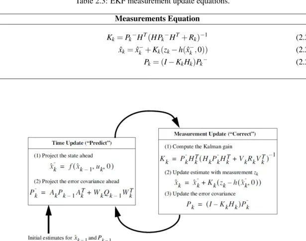
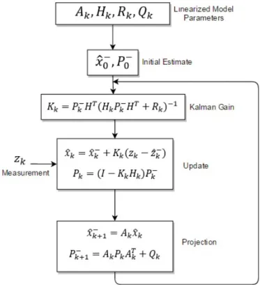
The complete set of EKF equations are shown in Tables 2.2 and 2.3. As with the basic discrete Kalman filter, the time update equations in table 2.2 project the state and covariance estimates from the previous time step k − 1 to the current time step k. Again, f in equation 2.18 comes from equation 2.7, Akand Wkare the process Jacobians at step k, and Qkis the process noise covariance

equation 2.3 at step k.

As with the basic discrete Kalman filter, the measurement update equations in table 2.3 correct the state and covariance estimates with the measurement zk. Again, h in equation 2.21 comes from

equation 2.8, Hkis the measurement Jacobian at step k, and Rkis the measurement noise covariance

The basic operation of the EKF is depicted in Figure 2.8. An important feature of the EKF is that the Jacobian Hk in the equation for the Kalman gain Kk serves to correctly propagate or

“magnify” only the relevant component of the measurement information. For example, if there is not a one-to-one mapping between the measurement zk and the state via h, the Jacobian Hkaffects

the Kalman gain so that it only magnifies the portion of the residual zk− h( ˆxk, 0) that does affect

the state. Obviously, if over all measurements there is not a one-to-one mapping between the measurement zkand the state via h, then as it might be expected, the filter will quickly diverge. In

this case the process is unobservable [34].

Table 2.2: EKF time update equations. Update Equations

ˆ

xk−= f ( ˆxk−1−, 0) (2.18)

Pk−= AkPk−1AkT+ Qk−1 (2.19)

Table 2.3: EKF measurement update equations. Measurements Equation

Kk= Pk−HT(HPk−HT+ Rk)−1 (2.20)

ˆ

xk= ˆx−k + Kk(zk− h( ˆx−k, 0)) (2.21)

Pk= (I − KkHk)Pk− (2.22)

respect to a reference frame [29, 35]. Thus, two different coordinate frames are considered:

• Earth Reference Frame - The earth frame E is represented by the orthogonal vector basis x0, y0, z0and is attached to the earth. Therefore, x0points north, y0points east and z0points

toward the center of earth as shown in Figure 2.9. This coordinate system is always static independently of the orientation of the body.

• Sensor Frame - The sensor frame S is rigidly attached to the object whose attitude we would like to describe. This frame is fixed to the sensor, but varies relative to the Earth reference frame due to the sensor movement.

In the literature, there are different ways of representing the attitude between two coordinate frames and transforming vectors and coordinates from one coordinate frame to another [35]. The most efficient method to represent upper limb segments orientation is Quaternions [26].

Figure 2.9: Earth Reference Frame [29].

2.2.3.1 Quaternions

A quaternion is a four-dimensional complex number that can be used to represent the orientation of a rigid body or coordinate frame in three-dimensional space. An arbitrary orientation of frame Brelative to frame A can be achieved through a rotation of angle θ around an axisAˆr defined in frame A.

This is represented graphically in Figure 2.10 where the mutually orthogonal unit vectors ˆxA,

ˆ

yAand ˆzA, and ˆxB, ˆyBand ˆzBdefine the main axis of coordinate frames A and B respectively. The

quaternion describing this orientation,A_Bˆq, is defined by equation (2.23) where rx, ry and rzdefine

the components of the unit vectorAˆr in the x, y and z axes of frame A respectively. A leading subscript denotes the frame being described and a leading superscript denotes the frame this is

with reference to. For example,ABˆq describes the orientation of frame B relative to frame A andAˆr

is a vector described in frame A [27].

Quaternion arithmetics often requires that a quaternion describing an orientation is first nor-malized. It is therefore conventional for all quaternions describing an orientation to be of unit length. A quaternion with unity norm is referred to as unit quaternion and can be used to represent the attitude of a rigid body [27]. Therefore, the unit quaternion is represented in equation 2.23.

A Bˆq = h q1 q2 q3 q4 i = h cosθ 2 −rxsin θ 2 −rysin θ 2 −rzsin θ 2 i (2.23)

The quaternion conjugate, denoted by *, can be used to swap the relative frames described by an orientation. For example, BAˆq is the conjugate of ABˆq and describes the orientation of frame A

relative to frame B. The conjugate ofA_Bˆq is defined by equation (2.24).

A Bˆq ∗₌B Aˆq = h q1 −q2 −q3 −q4 i (2.24)

The quaternion product, denoted by ⊗, can be used to define compound orientations. For example, for two orientations described by A_Bˆq and_CBˆq, the compounded orientation A_Cˆq can be defined by equation (2.25). A Cˆq = B Cˆq ⊗ A Bˆq (2.25)

For two quaternions, a and b, the quaternion product can be determined using the Hamilton rule and defined as equation (2.26). A quaternion product is not commutative; that is, a ⊗ b 6= b ⊗ a. a ⊗ b = h a1 a2 a3 a4 i ⊗hb1 b2 b3 b4 i =       a₁b₁− a₂b₂− a₃b₃− a₄b₄ a1b2+ a2b1+ a3b4− a4b3 a1b3− a2b4+ a3b1+ a4b2 a₁b₄+ a2b3− a3b2+ a4b1       T (2.26)

A three dimensional vector can be rotated by a quaternion using the relationship described in equation (2.27). Av and Bv are the same vector described in frame A and frame B respectively where each vector contains a 0 inserted as the first element to make them 4 element row vectors.

B_{v =}A

A BR =    1 − 2q2₃− 2q2 4 2(q2q3− q1q4) 2(q2q4+ q1q3) 2(q2q3+ q1q4) 1 − 2q22− 2q24 2(q3q4+ q1q2) 2(q2q4− q1q3) 2(q3q4+ q1q2) 1 − 2q2₂− 2q2₃    (2.28)

Therefore, by transposing this explanation to the orientation estimation of a sensor, with equa-tion (2.27) a three dimensional vector that could be the IMU output, described in sensor frame, can be rotated by a quaternion, giving the same vector but described in the earth reference frame.

Quaternions are used to represent orientation to improve computational efficiency and avoid singularities. In addition, the use of quaternions eliminates the need for computing trigonomet-ric functions [36]. However, the main disadvantages of using unit quaternions are: that the four quaternion parameters do not have intuitive physical meanings, and that a quaternion must have unity norm to be a pure rotation. The unity norm constraint, which is quadratic in form, is particu-larly problematic if the attitude parameters are to be included in an optimization, as most standard optimization algorithms cannot encode such constraints [35].

To conclude, human body tracking using inertial sensors requires an attitude estimation fil-ter capable of tracking in all orientations. Singularities associated with Euler angles2make them unsuitable for use in body tracking applications. So, quaternions are an alternate method of orien-tation represenorien-tation, gaining popularity in the graphics community. Quaternion roorien-tation is more efficient than the use of rotation matrices and does not involve the use of trigonometric func-tions [37].

Figure 2.10: The orientation of frame B is achieved by a rotation, from alignment with frame A, of angle θ around the axisAr [38].

2_{The transformation from the body frame to the Earth frame is based on three angular rotations. These angular}

rotations can be represented as the Euler angles: rotation ψ around X -axis (yaw angle), rotation θ around Y -axis (pitch angle) and rotation φ around Z-axis (roll angle).

2.3

Position and Trajectory Reconstruction

Measurements of movement of body segments need to be performed outside the laboratory, with body mounted sensors like accelerometers, gyroscopes and magnetometers. This means that IMUs are suitable for measuring arm movements, since they are small enough to be attached to the upper and forearm without interfering with the subject’s movement [39].

A fundamental question is defining the places and parts of the body where the sensors are placed. One very common solution is applying the sensors in joints of interest, for instance, the ones explained in Section 2.1.1.1. Additionally, it has been observed that significant errors, e.g. rapid variations, quite often appeared in the measurements. This mainly results from the soft tissue effects and inertial properties, where the relative movements between the sensors and the rigid structures (i.e. bones) are sampled [40].

There is a considerable amount of studies that have used sensor fusion with accelerometers, gyroscopes, magnetometers or combinations of these in the determination of orientation and po-sition of upper limb anatomical segments with the purpose of tracking upper limb movement and reconstruct its trajectories. After finding the sensors orientations using sensor fusion techniques, the biomechanical models for the upper limb are used to reconstruct upper limb motion. Also, to determine the position of an arm in an earth reference frame, it is necessary to transform the inertial measurements from the sensor coordinate system to the earth reference frame. Figure 2.11 illustrates a moving inertial sensor and two engaged coordinated systems (or frames). To report positions in the earth reference frame, the orientation of the sensor relative to the earth needs to be known.

In Table 2.4 there is an overview of upper limb tracking related work by several authors. This table presents the work summarized in this section and other examples. The table is organized in terms of author, year, sensors, sensor location, kinematic model, orientation representation, sensor fusion method, position estimation and results. The sensors are the IMU sensors used in each work, and the sensor locations are the place where they are attached. The kinematic model is the upper limb model considered in each work and corresponds to the modeling of its joints and movements. The position estimation is related to the method that is used to obtain the upper limb positions and the reconstruction of its trajectories and is based on the joint orientation and on the kinematic model considered. Lastly, the results are the output from each work.

Considering Table 2.4, regarding the sensors, the MT-9, MT9-B and MT-X are frequent inertial sensors used in the upper limb motion tracking. The MT9 module consists of 3-D gyroscopes and 3-D accelerometers. The MTX and the MT9-B modules consists of 3-D gyroscopes, 3-D accelerometers, 3-D magnetometers, and a temperature sensor. A Sparkfun 9-DOF is composed by a tri-axis accelerometer, a tri-axis micro rate gyro and tri-axis micro magnetometer. In sensor fusion method, N/A means that no sensor fusion method was applied, instead an optimisation approach was used to reduced drift [41] [18]. In [19] a Monte Carlo Sampling based optimisation technique is used to correct drift problems. In the examples presented below, there is no concern in defining an upper limb reference frame because the sensor reference frames are already aligned

T able 2.4: Ov ervie w of upper limb motion tracking related w ork. A uthor Y ear Sensors Sensor Location Kinematic Model Orientation Repr esentation Sensor Fusion P osition Estimation Results R. Zhu Z. Zhou [22 ] 2004 2 ISP Upper and lo wer arm 1-DOF elbo w Joint angle and Rotation axis KF Global transfer matrix Lo wer arm end position H. Zhou H. Hu [42 ] 2005 1 MT9 Wrist 3-DOF shoulder+ 3-DOF elbo w Euler Angles Extended KF In v erse kinematics Elbo w and wrist positions H. Zhou et al [41 ] 2005 1 MT9 Wrist Rigid forearm (elbo w fix ed) Euler Angles N/A In v erse kinematics F orearm position H. Zhou et al [18 ] 2006 2 MT9 Elbo w and wrist 6-DOF shoulder + 1-DOF elbo w Euler Angles N/A Wrist and elbo w -Euler angles + Kinematic model Shoulder , elbo w and wrist positions Shoulder -Lagrange optimisation H. Zhou et al [19 ] 2006 1 MT9 Wrist 3-DOF shoulder + 1-DOF elbo w Euler Angles N/A Wrist -acceleration double inte gration Elbo w and wrist positions Elbo w -Euler angles + Kinematic model H. Zhou et. al [43 ] 2007 2 MTx Elbo w and wrist 1-DOF elbo w Quaternions KF Elbo w and wrist -kinematical modeling Shoulder , elbo w and wrist positions Shoulder -acceleration angular changes fusion H. Zhou H. Hu [40 ] 2007 2 MTx Upper arm and wrist 1-DOF elbo w Euler Angles KF Elbo w and wrist -kinematical modeling Elbo w and wrist positions H. Zhou et al [24 ] 2008 2 MT9-B Elbo w and wrist 1-DOF elbo w Euler Angles N/A Wrist and elbo w -Euler angles + Kinematic model Shoulder , elbo w and wrist positions Shoulder -Lagrange optimisation C. Chien et. al [44 ] 2013 2 Sparkfun 9-DOF Upper and lo wer arm 1-DOF elbo w Rotation Matrix Non-linear CF Orientation + Kinematic model Reconstruction of wrist mo v ement

sults, the relative transformation between the inertial sensor coordinate frames and the segment coordinate frames were ignored. Moreover, they usually require users to align the sensors with each other and with the mounted arm segment, which inhibits their implementation in daily life monitoring. In order to avoid this step, a simple sensor-to-body transformation method could be introduced.

In order for the positions and trajectories tracking to be independent of how the user places the sensors on each segment, it is necessary to define a global reference frame where the positions will be described. After defining this global reference frame, the orientation of each sensor relative to it must be determined.

This way, the final goal of the sensor-to-body transformation process is to find this orientation in order to describe each segment movement in the global reference frame.

Usually, the sensor-to-body transformation consists of defining a set of movements around the upper limb rotation axes for each joint. This procedure is done in order to understand how the sensor is placed and to determine the orientation relative to the defined global coordinate frame where the positions trajectories will be described. Once the global frame is constructed and knowing the orientation of the upper limb segments relative to it, the trajectories can be represented in a unique frame, independent of how the sensors were attached in the first place.

In literature, there are some example of sensor-to-body transformation procedures like the ones reported by H. Wang et al [45] in 2011 and Y. Wang et al [46] in 2014.

In a study developed by H. Wang et al [45] in 2011, the relative orientation between the inertial sensor coordinate frames and the segment coordinate frames were calibrated using the gravity and the sensor data while the subject performs several predefined actions. In the sensor-to-body transformation postures, data from accelerometers and gyroscopes were fused to extract the gravity using Extended Kalman Filter (EKF). Then, the calibrated relative orientation matrix was used to bridge the sensor orientation with the segment orientation, which was then used to track the upper limb motion.

Another sensor-to-body transformation method is presented in the work developed by Y. Wang et al [46] in 2014, where a simple sensor-to-body transformation method was introduced, which effectively avoided the burden of manually aligning the sensors. In addition, the algorithm auto-matically estimated the arm length so that position trajectories of the elbow and the wrist joints could be reconstructed without manual measurements.

With a sensor-to-body transformation process, it is possible to have a more accurate motion tracking and avoid the burden of manually aligning the sensors, allowing the use of the tracking system in daily life monitoring.

System

This Chapter presents the development of an inertial tracking system proposed for this dissertation. The tracking system developed was named 3DArm - Upper Limb Inertial Tracking System. In this Chapter, the methodology and processes for the implementation of this system will be described and it will be presented an evaluation of its performance. All the work developed was to track only the rigth upper limb, to track the left upper limb the methodology is equivalent.

3.1

3DArm Overview

The Upper Limb Inertial Tracking System (3DArm) is a sequential algorithm that was developed in order to obtain upper limb joint positions and trajectories in 3D. Based on literature review, a set of steps for 3DArm implementation was defined, which is depicted in Figure 3.1.

Data Acquisition, described in Section 3.2, is related to sensor signal acquisition. The sensors are placed on the upper and lower arm segments, which is explained in Kinematic Model and Global Body Reference Frame Section 3.2.2.

Signal Pre-Processing, explained in Section 3.3, is divided in two different processes: Low-Pass Filter, to remove high frequency noise, and Data Normalization, to define normalized accel-eration and angular velocity vectors.

Sensor to Global Body Reference Frame, addressed in Section 3.4, is introduced in order to obtain the orientation between the sensor’s local reference frame and the global body reference frame, enabling positions and trajectories to be represented in the global body reference frame. This step is outlined with a different color in the flowchart of Figure 3.1 because it describes a process based on a transformation between reference frames that occurs during the Orientation Estimation phase.

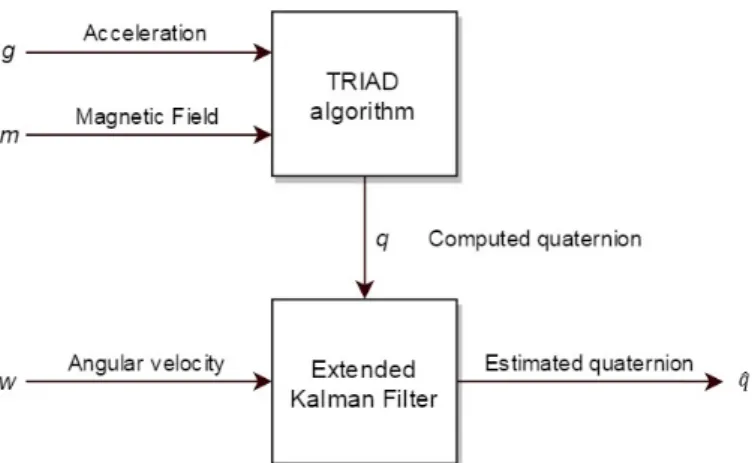
Orientation Estimation, detailed in Section 3.5, presents a sensor fusion method, EKF, that fuses data from accelerometers, gyroscopes and magnetometers, in order to obtain the orientation of each segment relative to the Global Body Reference Frame. This method was developed