Repositório ISCTE-IUL
Deposited in Repositório ISCTE-IUL: 2019-03-26
Deposited version: Post-print
Peer-review status of attached file: Peer-reviewed
Citation for published item:
Ramos, S., Vermunt, J. K. & Dias, J. G. (2011). When markets fall down: are emerging markets all the same?. International Journal of Finance and Economics. 16 (4), 324-338
Further information on publisher's website: 10.1002/ijfe.431
Publisher's copyright statement:
This is the peer reviewed version of the following article: Ramos, S., Vermunt, J. K. & Dias, J. G. (2011). When markets fall down: are emerging markets all the same?. International Journal of Finance and Economics. 16 (4), 324-338, which has been published in final form at
https://dx.doi.org/10.1002/ijfe.431. This article may be used for non-commercial purposes in accordance with the Publisher's Terms and Conditions for self-archiving.
Use policy
Creative Commons CC BY 4.0
The full-text may be used and/or reproduced, and given to third parties in any format or medium, without prior permission or charge, for personal research or study, educational, or not-for-profit purposes provided that:
• a full bibliographic reference is made to the original source • a link is made to the metadata record in the Repository • the full-text is not changed in any way
The full-text must not be sold in any format or medium without the formal permission of the copyright holders. Serviços de Informação e Documentação, Instituto Universitário de Lisboa (ISCTE-IUL)
When Markets Fall Down: Are Emerging
Markets All Equal?
Sofia B. Ramos ∗
ISCTE–Business SchoolJeroen K. Vermunt
Tilburg UniversityJos´e G. Dias
ISCTE–Business School AbstractThis paper studies the dynamics of stock market regimes in emerging economies. More specially, we show that it is incorrect to treat emerging markets as a single homogeneous group of markets because there is strong evidence for substantial differences in their regime-switching dynamics. For our analysis, we used a mixture or latent class version of the standard regime-switching model which classifies the analyzed emerging markets into three types of clusters. Whereas each of these three types of markets is characterized by the same two regimes – a bull state with positive returns and low volatility and a bear state with negative returns and high volatility – they clearly differ with respect to their regime-switching dynamics. The first class of stock markets moves fast between the two regimes, the second class shows more regime persistence, and the third class shows less likely than the others to switch to a bear regime period. There turn out to be no relationship between having a particular of these three types of regime-switching dynamics and regional characteristics of the economy concerned. The last part of the paper addresses regime synchronicity. We show that even though emerging markets exhibit some regime synchronicity that does not rule out presenting different dynamics in the regimes.
JEL classification: C22, G15
1 Introduction
Because emerging markets are thought to have an enormous growth poten-tial, they have drawn the attention of investors in the last decades. They are responsible for a dramatic expansion of the investment opportunities in the last decades and have been the main drivers of the diversification benefits of international investing (Goetzmann et al., 2005). The gains of emerging mar-kets did, however, come with certain costs. The recent history of emerging markets is full of episodes of price disruptions which are an important concern of investors.
It is well known that financial markets present upward and downward trends.1 Academics have tried to model these times series with disruptions in trends, among other with the regime-switching models (RSM) introduced by Hamilton (1989). The idea to characterize the state of a stock market in terms of regimes is especially relevant in emerging markets because in these markets financial crises tend to occur more often and to last longer than in developed markets, which strongly impacts the wealth of investors (see for instance Kole et al. (2006) for the implications of systemic crises on asset allocation decisions). In a general framework, Ang and Bekaert (2002a, 2004) show that regime-switching dynamics should be incorporated in asset allocation strategies. Although it is common to treat emerging markets as a single homogeneous financial asset class, there is substantial differences between these markets in many aspects, such as the regulations regarding international capital mobil-ity, political regimes, and exchange rates regimes. In this paper we question whether all emerging stock markets have similar regime-switching dynam-ics. Whereas dealing unobserved heterogeneity has proved to be important in many research areas, 2 in finance research heterogeneity has been mostly as-sumed observed: Groups and their boundaries are delineated a priori without taking into account the intrinsic information available in the observed data
∗ Address: Finance Department, IBS–ISCTE Business School, Av. For¸cas Ar-madas, Edif´ıcio ISCTE, 1649-026 Lisbon, Portugal, Tel. +351 217903977, Fax +351 217964710.
Email addresses: [email protected](Sofia B. Ramos),
[email protected](Jeroen K. Vermunt), [email protected] (Jos´e G. Dias).
1 A common terminology is to classify stock markets in “bull” and “bear” markets
according to market expectations. Bull markets correspond to a generalized upward trend (positive returns) and bear markets correspond to periods of a generalized downward trend (negative returns). Ang and Bekaert (2002a, 2004) label regimes as “normal” and “bear” markets.
2 As Heckman emphasized in his Nobel lecture (Heckman, 2001), one of the most
important discoveries in microeconometrics is the pervasiveness of heterogeneity and diversity in economic life.
on the process of interest. We question these heuristic approaches, as well as the presumption that emerging markets form a single homogeneous group. For an investor it is not only important to know what regimes investments might face, but even more important to know the likelihood that a certain asset switches to another regime. By expanding common RSMs we are able to classify countries with respect to their likelihood of switching between bear and bull regimes and the other way around.
Our paper is the first to address simultaneously the issue of heterogeneity in emerging markets as well as the existence of regimes. Previously, Edwards et al. (2003) analyzed stock market cycles in four Latin countries and two Asian countries to see whether they have similar features. They find that cycles in emerging markets tend to have shorter duration and larger amplitude and volatility than in developed countries. Their findings suggest a higher co-movement of stock markets after the liberalization process.
We propose using a new heterogeneous switching-regime model (HRSM) for financial econometric analysis that takes into account unobserved heterogene-ity by means of a time-constant discrete latent variable in addition to the time-varying discrete latent variables representing the regimes. The result la-tent class or mixture model is especially attractive in the context of the typical analysis in finance research because it yields a model-based clustering of ob-servational units. Here, this methodology is used to classify 18 emerging stock market indexes based on the dynamics of their returns.
The contributions of our research can be summarized as follows: First, we present the results of modeling regimes for emerging markets time series. 3 It turns out that emerging markets can be characterized by two regimes or states: a bear state with negative returns and high volatility and a bull state with positive returns and low volatility. This is in agreement with the results reported by Ang and Bekaert (2002a) who also found two regimes using data on the US, UK and Germany stock markets.
The second contribution is that we account for unobserved heterogeneity be-tween emerging markets. An investor would typically be interested in iden-tifying clusters of markets that differ in their propensities to specific charac-teristics, e.g. to switch between regimes. We investigate whether the common practice of the financial industry to cluster emerging markets regionally is suitable. For this purpose we expand the methodology of Hamilton (1989) by introducing a discrete latent variable capturing unobserved heterogeneity in RSMs. The latent class or finite mixture modeling methodology we pro-pose has proven to be a powerful tool for analyzing a wide range of social 3 Regime switching has already been applied for studying equity returns of
devel-oped markets (Ang and Bekaert, 2002a), interest rates (Ang and Bekaert, 2002b) and exchange rates (Kanas, 2005).
and behavioral science data (see, for example, McLachlan and Peel (2000)). A striking feature captured by the new model is that stock markets that are similar with respect to their regimes may differ substantially in their dynam-ics; that is, in the likelihood of jumping from one regime to another. Based on our results the hypothesis of a regional clustering should be rejected. It turn out that the sample of countries can be divided into three classes with dif-ferent regime-switching dynamics. Whereas all groups show a certain amount of regime persistency, one group of emerging markets is more likely to switch into bear regimes. In another class, we find countries with a lower propensity to switch to this regime. The third class contains the emerging stock markets that are more dynamic, moving faster between regimes. The traditional RSM model fails to recognize the different regime-switching dynamics by assuming the same change pattern in all 18 stock markets.
Third, we investigate stock market synchronization using various types of measures. Countries such as Chile, Czech Republic, Peru, Philippines and South Africa show a high level of general synchronicity with other emerging markets. On the other extreme, we find countries such as India, Israel and Pakistan that show a low level of coincidence with other emerging markets regime. An interesting feature of our analysis is that the association with other emerging markets regimes does not preclude countries from having different regime-switching dynamics; that is, to belong to different clusters. A good illustration is the case of Chile, which shows a large co-movement with its neighbors, Argentina and Brazil: when the Chilean market is in a bear regime, the above neighbors are in that regime as well. However, the jump to bull market is faster than its neighbors.
A last remark we would like to make is that the proposed methodology ac-counts for the problem of non-normality in financial returns. It is well docu-mented that emerging markets’ returns are not normally distributed (see for instance Harvey (1995), Bekaert et al. (1998) or Susmel (2001)). As indicated above, the proposed heterogeneous regime-switching model (HRSM) allows taking into account both stock markets between heterogeneity and hidden regimes within time series. But the flexible modeling of observed responses using a mixture of normal distributions makes it straightforward to capture almost any departure from the normality. Parameter estimation using the max-imum likelihood method is achieved by a generalization of the Baum-Welch algorithm.
The paper is organized as follows. Section 2 formulates the hypotheses that will be tested. Section 3 describes the 18 country financial time series data set that is used throughout this paper. Section 4 presents the heterogeneous regime switching model (HRSM) for the analysis of heterogeneous financial time series, as well as discusses shortly parameter estimation by maximum likelihood and model selection issues. Section 5 reports the results obtained
for the data set at hand. The paper concludes with a summary of the main findings and a description of possible implications.
2 Hypotheses
The label “emerging market”4 requires not only that a country has a low GDP per capita, but also that capital markets already reached a minimum threshold in terms of market capitalization. Because they are in early stage of development, emerging stock markets tend to present low liquidity, low mar-ket capitalization, concentration of stock marmar-kets in few companies – usually manufactures, communications and facilities – and highly regulated financial systems.
Often viewed as a financial asset class, emerging stock markets are charac-terized by high returns, high volatility and high diversification benefits, as they show low correlation with stock market indices of developed markets5. However, there exist substantial differences between the emerging markets in aspects such as regulation regarding international capital mobility, market size and liquidity, political regimes, and exchange rates regimes.
A strand of research has studied the effects of liberalization on emerging mar-kets. Table 1 reports liberalization dates for the countries studied by Bekaert and Harvey (2000). Most of these countries liberalized stock markets in the end of the eighties, beginning of the nineties. Only Hungary and South Africa liberalized later (in 1996). The table also reports other indicators frequently used to capture the openness of stock markets to foreign investors: the date of the introduction of the first ADR and the first country fund. In an analysis of equity returns of these emerging markets before and after financial reforms, Bekaert and Harvey (2000) found the correlation with developed countries in-creases and the volatility slightly dein-creases after liberalization. Furthermore, Edwards et al. (2003) found that liberalization processes contributed to a much stronger co-movement of the stock markets in emerging markets as measured by concordance indices and correlation of returns. Their main conclusion was that after reforms emerging markets became more integrated with one another. Based on the results of these two studies, one could argue that emerging mar-kets are an homogenous group of countries. This is the first hypothesis that will be investigated in this study.
Typically, the members of the class of emerging markets are grouped by ge-4 See International Finance Corporation (www.ifc.org).
5 For a review of emerging markets literature, see Errunza (1997) and Bekaert and
ographical areas. An example of this practice in the financial industry can be seen in the MSCI sub-indices on emerging markets which are clustered regionally6 because of the presumption that neighbor countries share certain important features. This idea is based on the fact that neighbor countries have more intense trade and, as a result, “cycles” related to one neighbor are likely to affect the other neighbor country. For example, when a country experiences a crisis marked by a currency depreciation, its major partners are negatively affected both through loss of competitiveness and through the fall in demand in the crisis country. The second hypothesis that will be investigated in this study is whether it is indeed the case that neighbor countries have similar regime-switching propensities.
[Table 1 about here.]
3 Description of the data set
We selected data on emerging markets that belong to the MSCI Emerging Market Index as of June 2006, as they represent the most active markets. These countries are Argentina, Brazil, Chile, China, Czech Republic, Hungary, India, Israel, Malaysia, Mexico, Pakistan, Peru, Philippines, Poland, Russia, South Africa, Taiwan and Thailand.
As noted by Goetzmann and Jorion (1999), many of the so-called “emerg-ing markets” are “re-emerg“emerg-ing markets”, markets whose stock markets have started a long time ago, but whose development was interrupted. More specif-ically, they indicated that many countries7 that already had active equity markets in the 1920’s experienced trading interruptions due to events such as wars, expropriations, hyperinflation, and political changes. As a result of this, a common problem in studying financial time series of emerging mar-kets is the availability of long time series. Although we collected data starting from 1985, for some countries complete data is only available from a later starting year. Hence, the data set used in this article are daily closing prices from 4 July 1994 to 31 July 2007 for the above emerging stock market in-dexes drawn from Datastream database8. The series are denominated in US dollars. In total, we have 3412 end-of-the-day observations per country. Let Pit be the observed daily closing price of market i on day t, i = 1, ...n and t = 0, ..., T . The daily rates of return are defined as the percentage rate of 6 These are the MSCI Emerging Markets (EM) Latin America Index and the MSCI
EM Europe, Middle East and Africa Index.
7 For instance, China, Malaysia, India, Egypt, Poland, Romania, Czechoslovakia,
Colombia, Uruguay, Chile, Venezuela and Mexico.
return by yit = 100 × log(Pit/Pi,t−1), t = 1, ..., T , with T = 3411. This defini-tion which is commonly used in the literature is justified by the fact that for expected small increases (decreases) of value, say r, log(1 + r) ' r.
The 18 stock markets in our sample are listed in Table 2, which also provides relevant descriptive statistics for the stock-return time series. Figure 1 depicts the full time series.
[Table 2 about here.] [Fig. 1 about here.]
The period analyzed can be characterized as a period of market instabil-ity. Although financial crises do not happen exclusively in emerging markets (see Sachs et al. (1996) and Kaminsky et al. (1998)), they are more frequent in emerging markets than in developed markets, and they usually have a larger negative impact. Moreover, crises in emerging markets tend to last longer than in developed markets (Patel and Sankar, 1998), and they tend to spread to all emerging markets in the region. The sample period includes the Mexican crisis of 1994, the East Asian Crisis of 1997, the Russian crisis of 1998, the 1999 Brazilian crisis, the Argentina crises in 2001-2002, as well as the global stock market downturn of the 2001 Internet bubble.
The descriptive statistics in Table 2 show that the mean return rates are all positive, except for Thailand. Central and Eastern European stock markets, such as Russian Federation, Hungary and Czech Republic, tend to have larger positive mean return rates than the other countries. Based on the median, one would however conclude that non-European stocks such as Mexico, Brazil and South Africa have the highest returns.
The analyzed markets show very diverse patterns of dispersion, where the largest standard deviation is found in Russian Federation (43.11%) and the lowest in Chile with a standard deviation of 16.42%. These differences in dis-persion of volatility are smaller than the ones found by Harvey (1995), who reported a difference of 86% between the lowest and the largest standard de-viation of returns in his emerging market sample, while in our data set the difference between the highest and the lowest standard deviation is around 35%. The smaller gap could be explained by the fact that, as shown in some studies (e.g. Bekaert and Harvey (2000)), volatility decreases after liberaliza-tion reforms.
Most of these stock market distributions of return rates are negative skewed, which can be explained by the series of market recessions in the studied pe-riod. Exceptions with positive skewness are Philippines, Russian Federation, Thailand and Peru. Moreover, the kurtosis (which equals 0 for normal dis-tributions) shows values above 0, indicating heavier tails and more peakness
than the normal distribution. The Jarque-Bera test rejects the null hypothesis of normality for each of the 18 stock markets. The non-normality of equity returns for stock markets has already been documented by Harvey (1995), Bekaert et al. (1998), and Susmel (2001).
4 The heterogeneous regime-switching model (HRSM)
Two different types of statistical methods have been proposed in the literature for identifying cycles or regimes in economic variables. The first type involves specifying a parametric model for the data generating process, where it is as-sumed that there is a switching between two regimes. While applications were initially in the analysis of business cycles (e.g. Goodwin (1993) and Diebold (1996)), more recently this approach was also used for the analysis of stock market dynamics (Hamilton and Lin (1996), Ramchand and Susmel (1998) and Maheu and McCurdy (2000)). The other alternative type of method is nonparametric: rather than specifying a statistical model that generated the data, it involves a search in the original time series for periods of general-ized upward and downward trends, as well as for turning points, peaks and troughs. Applications of this nonparametric approach in stock market analysis are reported by Pagan and Sossounov (2003) and Edwards et al. (2003). The HRSM for financial time series analysis that we describe next belongs to the first class of parametric methods.
Let yit represent the response of observation (stock market) i at time point t, where i ∈ 1, . . . , n, t ∈ 1, . . . , T , and yit ∈ <. This shows that we model simultaneously the time series of n stock markets. In addition to the observed “response” variable yit, the HRSM contains two different latent variables: a time-constant discrete latent variable and a time-varying discrete latent vari-able. The former, which is denoted by w ∈ {1, ..., S}, is used to capture the unobserved heterogeneity across stock markets; that is, stock markets are clus-tered based on differences in their dynamics. We will refer to a model with S clusters as HRSM-S. The two-state time-varying latent variable is denoted by zt ∈ {1, 2}. Changes between the two states or regimes between adjacent time points are assumed to be in agreement with a first-order Markov or first-order autocorrelation structure.
Let f (yi; ϕ) be the (probability) density function associated with the index return rates of stock market i. The HRSM-S defines the following parametric model for this density:
f (yi; ϕ) = S X w=1 2 X z1=1 2 X z2=1 · · · 2 X zT=1 f (w, z1, . . . , zT)f (yi; w, z1, . . . , xT). (1)
The right-hand side of this equation shows that we are dealing with a mixture model containing one time-constant latent variable and T time-varying latent variables. The total number of mixture components equals S · 2T, which is the product of the number of categories of w and zt for t = 1, 2, ..., T . As in any mixture model, the observed data density f (yi; ϕ) is obtained by marginalizing over the latent variables. Because in our model these are discrete variables, this simply involves the computation of a weighted average of class-specific probability densities – here f (yi; w, z1, . . . , zT) – where the (prior) class mem-bership probabilities or mixture proportions – here f (w, z1, . . . , zT) – serve as weights (McLachlan and Peel, 2000).
Using the factoring f (w, z1, . . . , zT) = f (w)f (z1, . . . , zT|w) and the assump-tion that within cluster w the sequence {z1, . . . , zT} is in agreement with a first-order Markov chain, we can simplify the form of f (w, z1, . . . , zT) as fol-lows: f (w, z1, . . . , zT) = f (w)f (z1|w) T Y t=2 f (zt|zt−1, w), (2) where
• f (w) is the probability of belonging to a particular latent class or cluster w with multinomial parameter πw = P (W = w);
• f (z1|w) is the initial-regime probability; that is, the probability of having a particular initial regime conditional on belonging to latent class w with Bernoulli parameter λkw = P (Z1 = k|W = w);
• f (zt|zt−1, w) is a latent transition probability; that is, the probability of being in a particular regime at time point t conditional on the regime at time point t − 1 and class membership; assuming a time-homogeneous transition process, we have pjkw = P (Zt = k|Zt−1 = j, W = w) as the relevant Bernoulli parameter. In other words, within cluster w one has the transition probability matrix
Pw = p11w p12w p21w p22w ,
with p12w = 1 − p11w and p22w = 1 − p21w. Note that the HRSM-S allows that each cluster has its specific transition or regime-switching dynamics, whereas in a standard RSM it is assumed that all cases have the same transition probabilities.
The other term in Equation (1) is the observed data density conditional on the latent variables, f (yi; w, z1, . . . , zT). As is typical in the literature on regime switching, we assume that the observed return at a particular time point de-pends only on the regime at this time point; i.e, conditionally on the latent state zt, the response yit is independent of returns at other time points, which is often referred to as the local independence assumption, and, moreover,
inde-pendent of the latent states occupied at other time points. These assumptions can be formulated as follows:
f (yi; w, z1, . . . , zT) = T
Y
t=1
f (yit; zt). (3)
The probability density of having a particular observed stock return in index i at time point t conditional on the regime occupied at time point t, f (yit|zt), is assumed to have the form of a univariate normal (or Gaussian) density func-tion. This distribution is characterized by the parameter vector θk = (µk, σk2) containing the mean (µk) and variance (σ2k) for regime k. Note that these parameters are assumed to be equal across clusters, an assuming that may, however, be relaxed. Since f (yi; ϕ), defined by Equation (1), is a mixture of densities across clusters w and regimes, it defines a flexible Gaussian mixture model that can accommodate deviations of normality in terms of skewness and kurtosis.
As far as the first-order Markov assumption for the latent regime switching conditional on cluster membership w is concerned, it is important to note that this assumption is not as restrictive as one may initially think. It does clearly not imply a first-order Markov structure for the responses yit. In fact, after marginalizing over w, the process for the sequence zt is not even Markovian. The standard regime-switching or hidden-Markov model (Baum et al., 1970; Hamilton, 1989; Ang and Bekaert, 2004) is the special case of the HRSM-S that is obtained by eliminating the time-constant latent variable w from the model, that is, by assuming that there is no unobserved heterogeneity. This model can be obtained without modifying the formulae, but by simply speci-fying that S = 1 yielding HRSM-1; that is, by assuming that all stock markets have homogeneous dynamics and belong to the same latent class. Whereas a general two-state HRSM-S has 4S + 3 free parameters to be estimated, includ-ing S − 1 class sizes, S initial-regime probabilities, 2S transition probabilities, 2 conditional means, and 2 variances, the two-state HRSM-1 has seven param-eters: one initial regime probability, two transition probabilities, two means and two variances.
Maximum likelihood (ML) estimation of the parameters of the HRSM-S in-volves maximizing the log-likelihood function: `(ϕ; y) = Pn
i=1log f (yi; ϕ), a problem that can be solved by means of the Expectation-Maximization (EM) algorithm (Dempster et al., 1977). In the E step, we compute f (w, z1, . . . , zT|yi) = f (w, z1, . . . , zT, yi)/f (yi), which is the joint conditional distribution of the T + 1 latent variables given the data and the current provisional estimates of the model parameters. In the M step, standard complete data ML methods are used to update the unknown model parameters using an expanded data matrix with f (w, z1, . . . , zT|yi) as weights. Since the EM algorithm requires us to compute and store the S·2T entries of f (w, z
market, computation time and computer storage increases exponentially with the number of time points, which makes this algorithm impractical or even impossible to apply with more than a few time points. However, for regime-switching or hidden-Markov models, a special variant of the EM algorithm has been proposed that is usually referred to as the forward-backward or Baum-Welch algorithm (Baum et al., 1970; Hamilton, 1989). This special algorithm is needed here because the model for our data set contains a huge number of entries in the joint posterior latent distribution f (w, z1, . . . , zT|yi). Recall that in our application T = 3411. This means that even for S = 2, the number of entries in the joint posterior distribution is too large to process and store for all n stock markets as has to be done within a standard EM algorithm. The Baum-Welch algorithm circumvents the computation of this joint posterior dis-tribution making use of the conditional independencies implied by the model. An extension of the Baum-Welch algorithm that includes the time-constant variable w is implemented in the Latent GOLD 4.5 software (Vermunt and Magidson, 2007) that we used to estimate the HRSM-S.
An important model selection issue is what value S should be. The typical approach would be to test a model with S − 1 clusters against a model S with clusters. However, this yields a likelihood ratio test with the null hypothesis defined on the boundary of the parameter space and as a result the asymptotic properties of the maximum likelihood estimates are no longer valid under the null hypothesis. Alternatively, the selection of S, the number of clusters needed to capture the unobserved heterogeneity across stock markets, can be based on information statistics such as the Bayesian Information Criterion (BIC) of Schwarz (Schwarz, 1978) and the Akaike Information Criterion (AIC) of Akaike (Akaike, 1974). Because simulation studies have shown that in mixture modeling AIC tends to overfit (see, for example, Dias and Vermunt (2007)), in our application we will select S that minimizes the value of BIC, which is defined as
BICS = −2`S( ˆϕ; y) + NSlog n, (4) where NS is the number of free parameters of the model.
5 Results
5.1 Regimes and clusters
This section reports the results obtained when applying the HRSM-S described in the previous section to the 18 stock markets. We estimated models using different values for S (S = 1, . . . , 8), where 1000 different starting values were used to avoid local maxima. A solution with three latent classes (S = 3) yielded the lowest BIC value (log-likelihood = -109177.894; number of free
parameters = 15, and BIC = 218399.144). This model will therefore be treated as the final model (HRSM-3). We also provide results for the HRSM-1 for comparison purposes.
Table 3 summarizes the results related to the distribution of stock market across latent classes which gives the size of each cluster. The estimated prior class membership probability is somewhat larger for Class 1 (0.442) and Class 2 (0.383) than for Class 3 (0.175). In simple words, it means that if we take this as representative sample of emerging markets the probability of finding an emerging market of Class 1 is larger than finding one of Class 2 and even of finding one of Class 3.
[Table 3 about here.]
A detailed interpretation of the nature of the latent class variable is obtained by investigating the posterior class membership probabilities, conditional on the observed data (Table 3). As can be seen, eight countries are assigned to Class 1, seven countries to Class 2 and the remaining 3 to Class 3. The results reject the hypothesis of regional clustering. Each of the three groups contains countries from different regions. The first group includes Argentina, Brazil, China, Pakistan, Poland, Russia, Taiwan and Thailand. The second group includes Czech Republic, Hungary, India, Israel, Mexico, Philippines, and South Africa, and the third and smaller group includes Chile, Peru and strikingly Malaysia. Except for Argentina and Hungary, the class assignments are always with probability one, indicating that the classes are almost fully nonoverlapped. Note that also for Argentina the misclassification probability is very low, assuming that we assign each stock market to the most likely latent class (modal class). The clusters contain countries with different liberalization dates.
If we combined this classification information with the descriptive statistics in Table 2, we see that Class 1 is a group that shows a wide range for the mean returns. Thailand has a negative return of 2.72% annually, while Russia rewards 29.41% annually during this period. The eight stock markets share a high volatility of around 30%, where Russia has the highest value with 40%. The second group is more homogeneous with respect to the mean and the volatility. All countries present positive average returns in the period, the average is 9.61% year, with Hungary presenting the highest value of 15.36%. The average volatility is around 25%, with values ranging between 21% and 28% year. Class 3 is quite heterogeneous in the following sense. It contains two neighbor countries, Chile and Peru, which present the lowest volatility of the sample, 16.42% and 18.25% respectively. Then it also contains Malaysia which has higher volatility, around 29%. From Figure 1, we can however observe that apart from the period of Asian crisis Malaysia’s stock market shows the same low volatility as Chile and Peru.
[Table 4 about here.]
Table 4 provides information on the two regimes that were identified; that is, the average proportion of markets in regime k over time and the mean and variance of the return in regime k. The reported means show that one of the regimes is associated with negative returns, around -37% if we convert to annual values, and the other with positive returns, around 23% annually. This corresponds to the typical distinction between bear and bull regimes. The probability of being in the bear and bull regimes is 0.237 and 0.763, respec-tively. We would also like to emphasize that these results are consistent with the common acknowledgment of asymmetry of the volatility in financial mar-kets. Volatility is likely to be higher when markets fall than when markets rise. The results are similar to the ones of Ang and Bekaert (2002a) who found two similar regimes for developed markets: a normal regime with positive returns and low volatility and bear regime with negative returns and high volatility. To gain more insight into the effect of applying the HRSM methodology, Table 4 also shows the regimes encountered with a standard RSM or HRSM-1; i.e., assuming homogeneity across all 18 emerging stock markets. The estimated regime-specific means and volatilities turn out to be similar irrespective of whether we assume homogeneity of transitions or not. The annual returns in the bear and bull regimes is again around -37% and 23%.
[Table 5 about here.]
Table 5 reports the estimated probabilities of beginning on one of the regimes for each latent class. The probability of initiating in the bear regime is smaller than the probability of initiating in the bull regime for all classes. Notwith-standing Class 1 has the largest probability of starting in this regime and Class 3 the smallest. This means that countries like Argentina, Brazil, China, Pak-istan, Taiwan, Thailand, Poland and Russia show a higher propensity to start in a bear regime than Mexico, India, Philippines, Czech Republic, Hungary, Israel and South Africa, which in turn have higher propensities than Chile, Peru and Malaysia. Note that Class 1 contains countries like Argentina, Brazil, Thailand or Russia that were severely affected by crises.
[Table 6 about here.]
Table 6 provides the key result of our analysis. It gives the transition prob-abilities between the two regimes for each of the three latent classes. First, notice that all classes show regime persistence. Once a stock market jumps to a regime it is likely to continue on it for some period. Second, Class 3 shows the lowest propensity to move from a bull regime to a bear regime. This propen-sity is higher for Class 2 and even higher for Class 1. Third, Class 2 shows the highest probability of jumping from a bear to a bull regime. We would like to highlight that the traditional RSM (or HRSM-1) does not account for these
important differences in the dynamics of switching regimes. Instead, by forcing the pattern of change to be the same in all 18 stock markets, one obtains a kind of average of the three sets of transition probabilities we found with the HRSM-3.
5.2 Stock markets dynamics and synchronization
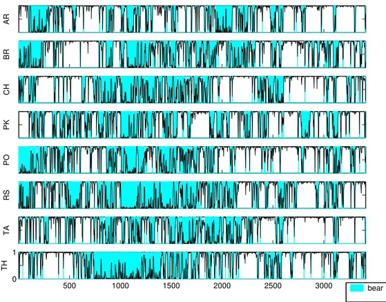
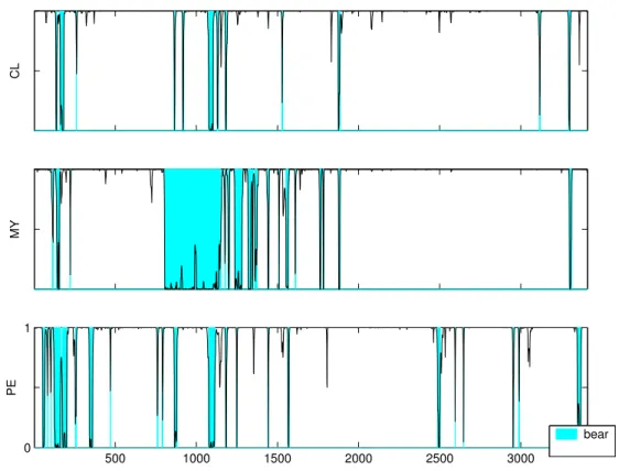
In this subsection we have a closer look at the synchronization of the regimes across markets. In order to hedge portfolio positions, for a risk averse investor it is relevant to know whether regime switches tend to coincide across emerging stock markets or whether they are more or less independent. Figures 2, 3, and 4 show the regime-switching dynamics of the countries within each of our three latent classes. These figures depict the posterior probability of being in bull regime at period t, where the blue color identifies periods in which this probability is below 0.5 which corresponds to a higher likelihood of being in the bear state.
[Fig. 2 about here.]
These figures show that the three clusters of countries have rather different pattern of regime switching. Emerging stock markets in Class 1 are extremely dynamic and tend to move very fast between regimes. Stock markets belong-ing to Class 2 are more regime persistent. This Class 2 contains markets with short duration crises that did not turn out to be endemic during the period of analysis. For concreteness, let us have a closer look at the cases of Poland and Hungary. These stock markets are similar in terms of mean return and volatil-ity, but are assigned to different classes. Looking again at Table 2, Poland has 11.4% of mean and 30% of volatility and Hungary has 15.5% of mean and 28% of volatility. However, Figure 2 shows clearly that Poland has a higher propensity than Hungary to fall in a bear regime, mainly in the beginning of the sample period.
Finally looking at profiles of the stock markets in Class 3, it can easily be seen why Malaysia belongs to this class. It turns out that the dynamic pattern of Malaysia is rather similar to Chile and Peru apart from the period of the Asian crisis in 1997. Similarly to Chile and Peru, after that period Malaysia shows no propensity to switch to a bear regime.
[Fig. 3 about here.] [Fig. 4 about here.] [Table 7 about here.]
Table 7 summarizes descriptive statistics – in columns, the mean, the first quartile, the median, the third quartile, and the inter quartile range – of regime durations in bear and bull markets for these emerging markets. Regime duration corresponds to the length in days in a given regime before switching into the opposite one.
A cursory look at the mean and median shows that the distribution of the durations is quite asymmetric both for bull and bear markets. Means are higher than median values. For instance, Argentina has for bear market an average duration of 10.4 while the median is 6. This implies the existence of episodic periods of bear regimes. For bear regimes the range of the median is between 5 and 7 days and countries do not exhibit strong differences. The third quartile has values between 9 and 16 days. Strikingly the mean value of Malaysia is substantially higher than in all others, that seems to be driven by a long episode of bear market.
When we look at bull markets the mean is also larger than the median re-vealing asymmetry. The median range goes from 11 days for China, Poland and Russia to 134 to Chile. The bull regimes median presents a lot of disper-sion which seems to be related with cluster membership. Among the countries with the lowest median are countries in Class 1, while countries with the largest median are the countries in Class 3. This analysis complements what we have learned until now from the methodology. The first class tends to have short regimes, both on bull and bear regimes. The second class shows more regime persistence, and the regime persistence is higher in bull markets. Class 3 presents the higher duration for bull regimes.
The final key issue we would like address is the synchronization of the regimes in which stock markets are at a particular time point. In order to measure synchronization and co-movements between the 18 emerging stock markets, we compute the Concordance Index (CI) introduced by Harding and Pagan (2002). The concordance between countries i and j is defined as
CIij = 1 T T X t=1 I(ˆzit= ˆzjt),
where I(A) = 1 if A is true and 0 otherwise. The index can be interpreted as the proportion of time units at which the two countries are in the same regime. It takes on values in the range between 0 (perfect mismatch) and 1 (perfect match). In practice, CIij will not become zero when two markets are fully independent. That is why it is better to use Cohen’s kappa coefficient as a measure of co-movement. This measure, which corrects CIij for the expected proportion of matches occurring by chance when the is no co-incidence at all, is defined as
κij =
CIij− P (e) 1 − P (e) ,
where P (e) is the probability that agreement is due to chance (Cohen, 1960). Maximum possible value of κijis 1 when CIij = 1 signifying perfect agreement; minimum possible κij is between 0 and −1 (when CIij = 0), signifying that agreement is less than can be attributed to chance; κij = 0 signifies that agreement is entirely attributable to chance.9
[Table 8 about here.]
Table 8 reports the concordance between emerging market regimes using these two measures. The above diagonal elements of the table contain CIij and the below diagonal elements contain κij. The CIij values range from 0.58 for Chile and Russia to 0.94 for Chile and Peru. The overall picture derived from these rather high values is that there seems to exist concordance of regimes in emerging markets. In particular, certain emerging markets show a high level of general synchronicity with other emerging markets. These are Chile, Czech Republic, Peru, Philippines and South Africa, for which CIijvalues are higher than 0.8 with various other markets. As an aside, note that these countries do all belong to Class 2 and Class 3.
The κij values below the diagonal range from -0.02 between Taiwan and Peru to 0.55 between Philippines and Malaysia. Argentina, Brazil and Mexico show mutual κij-based co-incidence values higher than 0.3. Though this indicates a certain tendency of regional synchronicity, this is counterbalanced by the regime synchronization between Mexico and both Czech Republic and Hun-gary. Chinese stock market regimes show some simultaneity with Philippines and Thailand, while the Thai stock market is associated with China, Malaysia and Philippines. The Polish market seems to co-move with Brazil, Hungary and Mexico, while South Africa co-moves with Czech Republic, Hungary and Mexico.
A popular approach to detect synchronization of stock markets is through cross correlation analysis. However, Edwards et al. (2003) refer that the use of cross correlations to study synchronicity of markets may be limited, because crises generate large “outliers” that introduce noise that blur the concordance between markets. Next we define a measure based on the correlation at regime level which filters out possible problems associated with extreme observations. Because the measures above incorporate uncertainty error due to the classifi-cation, we propose to use a measure of association between markets based on the posterior probability of being in a given regime. Let ˆαit be the estimated probability of market i at period t being in bull regime. Because they are
9 Because bull regimes occur more frequently for all the countries of the sample
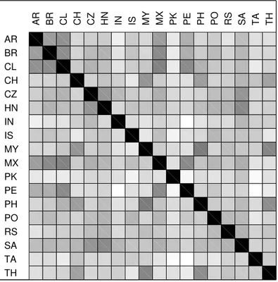
probabilities we apply the logit transformation to ˆαit: logitit= log ˆ αit 1 − ˆαit ! . [Fig. 5 about here.]
Figure 5 depicts the strength of the association between stock markets. It represents the absolute value of the correlation (the most negative value is -0.0115), i.e., the absolute correlation between logitit and logitjt. Therefore, the minimum and maximum correlation values (0 and 1) are colored with white and black, respectively. The gray colors for values in between are obtained by a linear grading of colors between white and black. The black diagonal means perfect correlation. Because there is only one negative correlation, it means that on general there is some coincidence on regimes.
We find clusters of countries with high correlation on the probability of shar-ing the same regime: Argentina, Brazil, Chile, Mexico and Peru. Also strong is the correlation between China, Malaysia, Philippines and Thailand. Then we also find a regime similarity between Poland and Hungary, and Hungary and Russia. Interesting is the alignment of South African stock market with Czech, Hungarian and Mexican stock markets. Countries that do not show any coincidence of regimes are India, Israel and Pakistan. The matrix shows that Chile, despite being in another group, is strongly associated with Argentina and Brazil. Therefore, despite different speed in dynamics through the period, there is still a large co-movement with its neighbors. Indeed, when the Chilean market is in a bear regime the big neighbors are in that regime as well. Inter-estingly, these results for Chile are in line with Edwards et al. (2003). They find that the Chilean economy is highly concordant with its close neighbors, Argentina and Brazil, but “at the same time it is somehow insured against contagion from crises that affect neighbors (p. 944)”. The same happens for Malaysia with Thailand. There is association between regimes but they belong to different classes as they show different dynamics in switching to regimes.
6 Conclusion
This research identifies regimes for emerging markets, and finds that the data is best described by two regimes. A bear regime, with negative returns and high volatility and a bull one, with positive returns and low volatility. This result is similar to Ang and Bekaert (2002a) who also find the same pat-tern return/volatility for data of US, UK and Germany. The identification of regimes is key in the field of portfolio management as portfolio optimization is dependent on key variables like expected returns and volatility.
As important as the identification of regimes is to know how emerging stock markets switch between regimes. We find that on general emerging markets show regime persistence, however they present some distinguished features. The first class of stock markets moves fast between the two regimes, the second class shows more regime persistence, and the third class is less likely than the others to switch to a bear regime period. There turn out to be no relationship between having a particular of these three types of regime-switching dynamics and regional characteristics of the economy concerned.
The paper also addresses stock market synchronization. Regime synchronic-ity exists among countries that are regionally closer but also among distant emerging markets. We shows that stock market synchronization of regimes does not preclude different dynamics in switching into regimes.
At last, we address what the paper does not attempt. The paper does not address contagion and financial crises. Similar to other studies that study cycles in stock markets (Ang and Bekaert (2002a) and Edwards et al. (2003)) we cannot establish a correspondence between bear regimes and crises, as well as we cannot conclude about contagion just because emerging markets are sharing the same regime. Stock markets can be sharing the same regime and we cannot disentangle whether is due to a bad macroeconomic situation or indeed because of contagion. Finally, what accounts for macro and financial fundamentals that explain the different dynamics for the different regimes is food for future research.
References
Akaike, H., 1974. A new look at statistical model identification. IEEE Transactions on Automatic Control, AC-19 716–723.
Ang, A., Bekaert, G., 2002a. International asset allocation with regimes shifts. Review of Financial Studies, 15(4), 1137–1187.
Ang, A., Bekaert, G., 2002b. Regimes switches in interest rates. Journal of Business and Economics Statistics, 20(2), 163–182.
Ang, A., Bekaert, G., 2004. How regimes affect asset allocation. Financial Analysts Journal, 60(2), 86–99.
Baum, L.E., Petrie, T., Soules, G., Weiss, N., 1970. A maximization technique occurring in the statistical analysis of probabilistic functions of Markov chains. Annals of Mathematical Statistics, 41, 164–171.
Bekaert,G., Erb, C., Harvey, C., Viskantas, T., 1998. Distributional char-acteristics of emerging market returns and asset allocation. Journal of Port-folio Management, Winter, 102–116.
Bekaert, G., Harvey, C., 2000. Foreign speculators and emerging equity markets. Journal of Finance, 55(April), 565–613.
Bekaert, G., Harvey, C., 2003. Emerging markets finance. Journal of Em-pirical Finance, 10, 3–55.
Bekaert, G., Harvey, C., Ludblad, C., 2005. Does financial liberalization spur growth?. Journal of Financial Economics, 77, 3–56.
Cohen, J., 1960. A coefficient of agreement for nominal scales. Educational and Psychological Measurement, 20, 37–46.
Dempster, A.P., Laird, N.M., Rubin, D.B., 1977. Maximum likelihood from incomplete data via the EM algorithm (with discussion). Journal of the Royal Statistical Society B, 39, 1–38.
Dias, J.G., Vermunt, J.K., 2007. Latent class modeling of website users’ search patterns: Implications for online market segmentation. Journal of Retailing and Consumer Services, 14(6), 359–368.
Diebold, F., Rudebusch, G. , 1996. Measuring business cycles: A modern perspective. The Review of Economics and Statistics, 78(1), 67–77.
Edwards, S., Biscarri, J.G., de Gracia, F.P., 2003. Stock market cycles, financial liberalization and volatility. Journal of International Money and Finance, 22(7), 925–955.
Errunza, V., 1997. Research on emerging markets: Past, present and fu-ture. Emerging Markets Quarterly, 1(3), 5–14.
Goetzmann, W., Jorion, P., 1999. Re-emerging markets. The Journal of Financial and Quantitative Analysis, 34(1), 1–32.
Goetzmann, W., Li, L., Rouwenhorst, K.G., 2005. Long-term global mar-ket correlations. The Journal of Business, 78, 1–38.
Goodwin, T.H., 1993. Business-cycle analysis with a Markov-switching model. Journal of Business & Economic Statistics, 11(3), 331-339.
Hamilton, J.D., 1989. A new approach to the economic-analysis of non-stationary time-series and the business-cycle. Econometrica, 57, 357–384.
Hamilton, J., Lin, G., 1996. Stock market volatility and the business cycle. Journal of Applied Econometrics, 11(5), 573–593.
Harding, D., Pagan, A., 2002. Dissecting the cycle: a methodological in-vestigation. Journal of Monetary Economics, 49(2), 365–381.
Harvey, C.R., 1995. Predictable risk and returns in emerging markets. Review of Financial Studies, 8, 773–816.
Heckman, J., 2001. Micro data, heterogeneity, and the evaluation of public policy: Nobel lecture. Journal of Political Economy, 109, 673–748.
Kaminsky, G.L., Reinhardt, C.M., 1998. Financial Crises in Asia and Latin America: then and now. American Economic Review, 88(2), 444–448. Kanas, A., 2005. Regime Linkages in the US/UK real exchange rate-real interest differential relation. Journal of International Money and Finance, 24(2), 257–274.
Kole, E., Koedijk, K., Verbeek, M., 2006. Portfolio implications of sys-temic risk. Journal of Banking and Finance, 30(8), 2347–2369.
Maheu, J., McCurdy, T., 2000. Identifying bull and bear markets in stock returns. Journal of Business & Economic Statistics, 18(1), 100–112.
Sons, New York.
Pagan, A.R., Sossounov, K.A., 2003. A simple framework for analysing bull and bear markets. Journal of Applied Econometrics, 18(1), 23–46.
Patel, S.A., Sankar., A., 1998. Crises in developed and emerging stock markets. Financial Analysts Journal, 54(6), 50–61.
Ramchand, L., Susmel, R., 1998. Volatility and cross correlation in global equity markets. Journal of Empirical Finance, 5(4), 397–416.
Sachs, J., Tornell, A., Velasco, A., 1996. Financial crises in emerging mar-kets: The lessons of 1995. Brookings Papers on Economic Activity, 1, 147– 217.
Schwarz, G., 1978. Estimating the dimension of a model. Annals of Statis-tics, 6, 461-464.
Susmel, R., 2001. Extreme observations and diversification in Latin Amer-ican emerging equity markets. Journal of International Money and Finance, 20(7), 971–986.
Vermunt, J.K., Magidson, J., 2007. LG-syntax user’s guide: Manual for Latent GOLD 4.5 syntax module. Belmont, MA: Statistical Innovations Inc.
List of Figures
1 Time series of index rates for 18 emerging stock markets 21 2 Estimated posterior bull regime probability and modal regime
within Class 1 22
3 Estimated posterior bull regime probability and modal regime
within Class 2 23
4 Estimated posterior bull regime probability and modal regime
within Class 3 24
5 Absolute correlation between posterior probabilities of being
1000 2000 3000 −200 20 AR 1000 2000 3000 −200 20 BR 1000 2000 3000 −200 20 CL 1000 2000 3000 −200 20 CH 1000 2000 3000 −200 20 CZ 1000 2000 3000 −200 20 HN 1000 2000 3000 −200 20 IN 1000 2000 3000 −200 20 IS 1000 2000 3000 −200 20 MY 1000 2000 3000 −200 20 MX 1000 2000 3000 −200 20 PK 1000 2000 3000 −200 20 PE 1000 2000 3000 −200 20 PH 1000 2000 3000 −200 20 PO 1000 2000 3000 −200 20 RS 1000 2000 3000 −200 20 SA 1000 2000 3000 −200 20 TA 1000 2000 3000 −200 20 TH
AR BR CH PK PO RS TA 500 1000 1500 2000 2500 3000 0 1 TH bear
Fig. 2. Estimated posterior bull regime probability and modal regime within Class 1
CZ HN IN IS MX PH 500 1000 1500 2000 2500 3000 0 1 SA bear
Fig. 3. Estimated posterior bull regime probability and modal regime within Class 2
CL MY 500 1000 1500 2000 2500 3000 0 1 PE bear
Fig. 4. Estimated posterior bull regime probability and modal regime within Class 3
AR BR CL CH CZ HN IN IS MY MX PK PE PH PO RS SA TA TH AR BR CL CH CZ HN IN IS MY MX PK PE PH PO RS SA TA TH
List of Tables
1 Dates of openness of emerging stock markets 27
2 Summary statistics 28
3 Estimated prior probabilities (P (W = w)), posteriord probabilities (P (W = w|yd i)) and modal classes for the
HRSM-3 29
4 Estimated marginal probabilities of the regimes and within
Gaussian parameters 30
5 Estimated initial distribution of the regimes (ˆλkw) 31 6 Estimated transition probabilities between regimes (ˆpjkw) 32
7 Estimated regime durations 33
8 Measures of market synchronization based on HRSM-3 (CIij
Table 1
Dates of openness of emerging stock markets
Official Liberalization Dates First First Country Bekaert and Harvey (2000) ADR Fund Argentina 1989 1991 1991 Brazil 1991 1992 1992 Chile 1992 1990 1989 China NA NA NA Czech Republic NA NA NA Hungary 1996 NA NA India 1992 1992 1986 Israel 1993 1987 1992 Malaysia 1988 1992 1987 Mexico 1989 1989 1981 Pakistan 1991 1994 1991 Peru 1992 1994 -Philippines 1991 1991 1987 Poland NA NA NA Russian Federation NA NA NA South Africa 1996 1994 1994 Taiwan 1991 NA NA Thailand 1987 1991 1985 This table presents dates of openness of stock markets to foreign investors: official liberalization dates from Bekaert and Harvey (2000), the introduction of the first American Depository Receipt (ADR) and the introduction of the first country Fund. Data is from Bekaert et al. (2005).
Table 2
Summary statistics
Annualised Daily
Stock Market Mean Standard Median Skewness Kurtosis Jarque-Bera test Deviation statistics p-value Argentina (AR) 0.6% 31.3% 7.9% -1.8 35.2 176800.11 0.000 Brazil (BR) 13.4% 31.5% 18.7% -0.2 5.1 3648.83 0.000 Chile (CL) 7.1% 16.4% 0.0% -0.1 3.3 1506.11 0.000 China (CH) 11.4% 29.8% 2.6% 0.0 5.2 3826.70 0.000 Czech Republic (CZ) 12.8% 21.3% 0.0% -0.2 2.4 874.33 0.000 Hungary (HN) 15.4% 27.8% 0.0% -0.7 10.0 14391.30 0.000 India (IN) 9.0% 25.0% 0.0% -0.4 4.8 3391.13 0.000 Israel (IS) 11.4% 22.2% 12.7% -0.5 4.8 3390.66 0.000 Malaysia (MY) 1.2% 29.4% 0.0% -1.6 74.5 786244.84 0.000 Mexico (MX) 9.4% 28.0% 20.8% -0.8 16.5 38895.91 0.000 Pakistan (PK) 2.8% 30.3% 0.0% -0.4 6.5 6008.90 0.000 Peru (PE) 11.5% 18.3% 8.0% 0.2 12.9 23689.12 0.000 Philippines (PH) 0.1% 24.8% 0.0% 0.9 16.1 37006.78 0.000 Poland (PO) 11.4% 29.9% 10.8% -0.1 3.2 1417.93 0.000 Russian Federation (RS) 29.4% 43.1% 12.0% 0.4 22.7 72822.49 0.000 South Africa (SA) 9.1% 23.8% 17.5% -0.8 6.9 7117.29 0.000 Taiwan (TA) 2.6% 27.1% 0.0% -0.1 3.2 1462.44 0.000 Thailand (TH) -2.7% 33.9% 0.0% 0.3 8.5 10207.31 0.000
Table 3
Estimated prior probabilities (P(W = w)), posterior probabilities (d P(W = w|yd i))
and modal classes for the HRSM-3
Stock market Latent Class 1 Latent Class 2 Latent Class 3 Modal Class
Prior probabilities 0.442 0.383 0.175 1 Posterior probabilities Argentina (AR) 0.995 0.005 0.000 1 Brazil (BR) 1.000 0.000 0.000 1 Chile (CL) 0.000 0.000 1.000 3 China (CH) 1.000 0.000 0.000 1 Czech Rep. (CZ) 0.000 1.000 0.000 2 Hungary (HN) 0.070 0.930 0.000 2 India (IN) 0.000 1.000 0.000 2 Israel (IS) 0.000 1.000 0.000 2 Malaysia (MY) 0.000 0.000 1.000 3 Mexico (MX) 0.000 1.000 0.000 2 Pakistan (PK) 1.000 0.000 0.000 1 Peru (PE) 0.000 0.000 1.000 3 Philippines (PH) 0.000 1.000 0.000 2 Poland (PO) 1.000 0.000 0.000 1 Russian Fed. (RS) 1.000 0.000 0.000 1
South Africa (SA) 0.000 1.000 0.000 2
Taiwan (TA) 1.000 0.000 0.000 1
Table 4
Estimated marginal probabilities of the regimes and within Gaussian parameters
HRSM-1 HRSM-3
Regime 1 Regime 2 Regime 1 Regime 2
P(Z) 0.239 0.761 0.237 0.763 (0.008) — (0.024) — Return -0.143 0.089 -0.141 0.088 (0.026) (0.005) (0.027) (0.005) Risk 9.295 1.057 9.357 1.037 (0.154) (0.012) (0.154) (0.012)
Table 5
Estimated initial distribution of the regimes (ˆλkw)
HRSM-1 HRSM-3
Latent class 1 Latent class 2 Latent class 3
Regime 1 Regime 2 Regime 1 Regime 2 Regime 1 Regime 2 Regime 1 Regime 2
0.245 0.755 0.409 0.591 0.180 0.820 0.052 0.948
Table 6
Estimated transition probabilities between regimes (ˆpjkw)
HRSM-1 HRSM-3
Latent class 1 Latent class 2 Latent class 3
Regime 1 Regime 2 Regime 1 Regime 2 Regime 1 Regime 2 Regime 1 Regime 2
Regime 1 0.912 0.088 0.894 0.106 0.889 0.111 0.929 0.071
(0.004) — (0.006) — (0.008) — (0.011) —
Regime 2 0.027 0.973 0.055 0.945 0.025 0.975 0.007 0.993
Table 7
Estimated regime durations
Countries Bear regime Bull regime
Mean Q1 Median Q3 IQR Mean Q1 Median Q3 IQR
Argentina (AR) 10.4 3.0 6.0 12.0 9.0 29.0 5.0 12.0 37.0 32.0 Brazil (BR) 12.0 3.0 7.0 16.0 13.0 24.2 6.0 13.0 31.0 25.0 Chile (CL) 8.0 2.5 5.0 9.0 6.5 255.0 46.5 134.0 344.5 298.0 China (CH) 10.8 3.0 6.0 13.5 10.5 24.0 5.0 11.5 22.0 17.0 Czech Republic (CZ) 9.0 2.0 6.0 12.0 10.0 56.8 10.5 30.5 62.0 51.5 Hungary (HN) 10.5 2.0 6.0 16.5 14.5 38.4 10.0 17.0 47.0 37.0 India (IN) 11.0 3.0 7.0 13.0 10.0 53.4 12.0 31.0 71.0 59.0 Israel (IS) 8.2 2.0 6.0 11.0 9.0 51.5 8.0 24.0 64.0 56.0 Malaysia (MY) 28.3 3.0 7.0 14.5 11.5 152.7 22.0 43.0 99.0 77.0 Mexico (MX) 13.4 2.0 7.0 15.0 13.0 55.0 9.0 21.0 45.0 36.0 Pakistan (PK) 9.9 2.0 5.0 13.0 11.0 22.4 5.0 12.5 28.0 23.0 Peru (PE) 10.3 2.0 4.5 16.0 14.0 138.5 33.0 68.0 192.0 159.0 Philippines (PH) 9.5 2.0 5.0 11.5 9.5 54.9 7.5 18.0 57.5 50.0 Poland (PO) 9.6 2.0 5.0 11.0 9.0 22.3 7.0 11.0 25.0 18.0 Russian Fed. (RS) 15.1 3.0 7.0 15.5 12.5 20.1 6.0 11.0 22.0 16.0
South Africa (SA) 10.0 3.0 6.0 12.0 9.0 58.2 10.0 29.5 60.0 50.0
Taiwan (TA) 10.1 2.0 6.0 15.0 13.0 26.1 7.0 13.5 27.0 20.0
Table 8
Measures of market synchronization based on HRSM-3 (CIij above the diagonal
and κij below the diagonal)
Countries AR BR CL CH CZ HN IN IS MY Argentina (AR) 1.00 0.72 0.76 0.65 0.73 0.69 0.69 0.72 0.70 Brazil (BR) 0.33 1.00 0.69 0.64 0.71 0.70 0.66 0.70 0.67 Chile (CL) 0.13 0.10 1.00 0.70 0.87 0.80 0.82 0.86 0.85 China (CH) 0.14 0.17 0.08 1.00 0.70 0.68 0.72 0.66 0.74 Czech Republic (CZ) 0.17 0.24 0.17 0.17 1.00 0.81 0.81 0.82 0.80 Hungary (HN) 0.15 0.26 0.11 0.18 0.34 1.00 0.75 0.76 0.76 India (IN) 0.11 0.14 0.03 0.26 0.25 0.19 1.00 0.77 0.77 Israel (IS) 0.16 0.21 0.15 0.08 0.22 0.19 0.11 1.00 0.77 Malaysia (MY) 0.10 0.14 0.13 0.29 0.19 0.20 0.13 0.07 1.00 Mexico (MX) 0.32 0.41 0.19 0.21 0.34 0.32 0.28 0.23 0.24 Pakistan (PK) 0.16 0.11 0.03 0.08 0.14 0.19 0.10 -0.03 0.15 Peru (PE) 0.20 0.16 0.29 0.06 0.15 0.06 -0.04 0.11 0.11 Philippines (PH) 0.18 0.19 0.19 0.30 0.23 0.22 0.13 0.15 0.55 Poland (PO) 0.20 0.32 0.09 0.19 0.24 0.32 0.16 0.20 0.17 Russian Fed. (RS) 0.11 0.16 0.03 0.20 0.19 0.20 0.15 0.12 0.18
South Africa (SA) 0.20 0.25 0.15 0.19 0.39 0.37 0.26 0.15 0.23
Taiwan (TA) 0.20 0.19 0.04 0.19 0.11 0.13 0.15 0.09 0.12 Thailand (TH) 0.10 0.11 0.06 0.38 0.11 0.18 0.21 0.05 0.38 Countries MX PK PE PH PO RS SA TA TH Argentina (AR) 0.76 0.66 0.76 0.73 0.68 0.59 0.73 0.68 0.62 Brazil (BR) 0.76 0.61 0.70 0.69 0.70 0.60 0.71 0.65 0.60 Chile (CL) 0.83 0.69 0.94 0.87 0.72 0.58 0.86 0.72 0.66 China (CH) 0.70 0.61 0.69 0.74 0.66 0.62 0.70 0.66 0.72 Czech Republic (CZ) 0.82 0.69 0.84 0.81 0.73 0.64 0.85 0.70 0.66 Hungary (HN) 0.78 0.69 0.76 0.77 0.74 0.63 0.81 0.67 0.66 India (IN) 0.78 0.67 0.78 0.77 0.69 0.62 0.80 0.70 0.68 Israel (IS) 0.79 0.63 0.83 0.79 0.71 0.60 0.79 0.69 0.63 Malaysia (MY) 0.78 0.69 0.83 0.89 0.70 0.63 0.80 0.70 0.76 Mexico (MX) 1.00 0.70 0.83 0.80 0.74 0.66 0.81 0.71 0.68 Pakistan (PK) 0.20 1.00 0.68 0.69 0.64 0.60 0.69 0.60 0.61 Peru (PE) 0.26 0.04 1.00 0.84 0.71 0.57 0.82 0.69 0.64 Philippines (PH) 0.29 0.15 0.17 1.00 0.72 0.62 0.81 0.71 0.74 Poland (PO) 0.31 0.15 0.11 0.22 1.00 0.66 0.72 0.64 0.63 Russian Fed. (RS) 0.24 0.16 0.01 0.14 0.29 1.00 0.63 0.64 0.66
South Africa (SA) 0.33 0.14 0.07 0.25 0.21 0.18 1.00 0.70 0.67
Taiwan (TA) 0.19 0.02 -0.02 0.16 0.13 0.23 0.12 1.00 0.65