Exchange Market Pressure in African Lusophone Countries
1Jorge Braga de Macedo,2 Luís Brites Pereira3 & Afonso Mendonça Reis4
14 September 2007
Abstract
This paper explores the credibility of exchange rate arrangements for the five African Portuguese-speaking (PALOP) countries. Our working hypothesis is that credibility necessarily implies low mean exchange market pressure (EMP), low EMP conditional volatility and low-severity EMP crises. In addition, economic fundamentals must account for EMP dynamics. We also seek evidence of a risk-return relationship for mean EMP and of “bad news” (negative shocks) having a greater impact on EMP volatility than “good news” (positive shocks). Using our econometric models, we are able to rank PALOP countries’ conditional volatility in ordinal terms. Our main conclusion is that countries with currency pegs, such as Guinea-Bissau (GB) and Cape Verde (CV), clearly have lower volatility when compared to those with managed floats and are therefore more credible. Moreover, EMP crises episodes under pegs are much less severe. We find that economic fundamentals correctly account for mean EMP in all countries and that the risk-return relationship is much more favourable for investors under currency pegs, as the increase in volatility is lower for the same rate of return. The exception to this finding is Mozambique (MOZ), which apparently has a risk-return profile akin to that enjoyed by countries with pegs. A plausible reason is that MOZ has the only managed float in our sample implementing monetary and exchange rate policy within the confines of an IMF framework, which establishes floors for international reserves and ceilings for the central bank’s net domestic assets. This intuition needs to be tested, however. EMP conditional volatility is generally driven by changes in domestic credit (lowers it) and foreign reserve changes (raises it). The first effect is more pronounced under currency pegs, but also under MOZ’s managed float. “Bad news” increases volatility more that “good news” only in the case of CV’s currency peg, which we take to be another sign of its credibility. A few striking cross-country comparisons also emerge in our analysis. Among countries with managed floats, we find that Angola (ANG) has the most severe EMP crises whilst MOZ has the least severe. São Tomé & Princípe (STP), meanwhile, lies between these two extremes but its EMP crises behaviour is clearly much closer to that of MOZ. STP’s credibility may also be improving since its volatility has declined as of 2002 and its level is now much closer to that of MOZ, whose managed float has lowest volatility of such arrangements.
Keywords: Exchange Rate Regime, Exchange Market Pressure, EGARCH-M
JEL Classification: C22, F31, F33
1First draft of paper to be presented at the African Economic Conference 2007 in Addis Ababa, Ethiopia on 15-17
November.
2
Professor of Economics at Nova University, President of the Tropical Research Institute (IICT), both in Lisbon.
3
Assistant Professor, Faculty of Economics at Nova University and Research Fellow of the Tropical Research Institute (IICT), both in Lisbon. Corresponding author’s email address: lpereira@fe.unl.pt
4
1. Introduction
Global financial markets change the environment for economic policymaking, most visibly in the choice of exchange rate regime. When capital markets are integrated, the main issue becomes that of the relative importance attached to exchange rate stability and domestic monetary independence. At the heart of this issue is the so-called “impossible trinity” dilemma, which holds that a country can only attain two of the following three goals simultaneously: exchange rate stability, monetary independence and financial-market integration. Monetary independence is clearly greater under floating exchange rates, as the value of a currency is allowed to vary continuously in response to prevailing exchange market pressure (EMP), which reflects the excess demand for a currency arising when the total value of foreign goods and assets demanded by domestic residents is higher than that demanded by foreigners at the prevailing exchange rate. However, the benefit of greater independence has to be balanced against the cost of greater volatility and uncertainty in real exchange rates.
For many developing countries, limiting exchange rate variability by fixing a domestic currency’s value to that of a sounder foreign currency is often seen as desirable. The reason is that fixing the exchange rate provides a nominal anchor that has two important benefits. First, it fixes the inflation rate for internationally traded goods, and so contributes to controlling inflation. Second, it anchors domestic inflation expectations to the anchor country’s inflation rate. As a result, domestic inflation falls in line with that of the anchor country, as do interest rates. Under free capital mobility, a credible currency-peg implies that a country has in effect adopted the anchor country’s monetary policy and, consequently, its low expected inflation. Under fixed exchange rates, the burden of adjustment to prevailing EMP thus falls exclusively on foreign reserves and interest rate changes.
With respect to intermediate arrangements, a major policy debate in the literature is whether these are viable or not. Under such arrangements, EMP is relieved by some combination of changes in the exchange rate, in foreign reserves and in domestic credit. The focus on intermediate arrangements is particularly relevant given that almost all currency crises in the past decade took place against a background of fixed but adjustable exchange rates, i.e. arrangements allowing a step change in the value of a currency as a result of a discretionary decision by domestic monetary authorities.
It is noteworthy that currency crises often became financial crises as sovereign credit ratings plummeted and access to international capital was lost following a currency’s collapse. In this regard, the East Asian “twin” financial and currency crashes of the 1990s underscored the relative ease with which it was possible to implement the “wrong” combination of currency pegs and economic policy under a given degree of financial-market integration. The commitment of authorities who seek exchange rate stability, through the adoption of fixed but adjustable exchange rate regimes, is therefore likely to be tested under financial-market integration.5 More recently, this policy debate has become more prominent in connection with the so-called “benign peg” of the Chinese currency to the US dollar.6
5
The relevance of the European Payments Union is pointed out in Braga de Macedo & Eichengreen (2001c). The “Eurocentric” view has been presented as evidence of an intermediate exchange rate system which helps acquire financial reputation and is applied to the Franc zone and to Latin America in Braga de Macedo, Cohen & Reisen (2001b). The “Eurocentric” view essentially extends an interpretation of the first European attempts at promoting a multilateral payments system into an argument for improving regional monetary and fiscal surveillance. While the quantitative relevance of multilateral surveillance to international lenders and credit rating agencies’ scrutiny has not been tested directly, the European experience does signal when it is bound to be especially intense.
6
Indeed, a possible explanation of the current international monetary system goes back to the Bretton Woods system. This was discussed at a conference at the University of Santa Cruz in May 2006 on “The Euro and the
The literature also highlights the consensual view that policymakers will always have to take into account financial markets’ responses to their policy actions in seeking an optimal trade-off between exchange rate stability and domestic monetary independence. After a country has chosen its exchange rate policy regime (fixed, floating, or fixed-but-adjustable) under a given degree of financial market integration, it then has the task of adapting its domestic economic policy and institutional environment in accordance with that choice. Indeed, the extent to which it is able to establish a credible interaction between a country’s financial-market integration, exchange rate arrangements and the accompanying policy and institutional responses will be paramount in establishing its reputation in international financial markets.7
For any country, establishing financial reputation is important for two reasons: First, it leads to a low-risk borrower profile and improved credit terms when seeking foreign capital, as reflected in its international credit rating. Second, it is conducive to low and more stable domestic interest rates, especially under fixed exchanges. Given that interest rates are an inter-temporal price, and, as such, heavily influenced by agent’s expectations, low interest rate spreads are considered to be an indicator of financial reputation.
The range of reforms required to establish financial reputation is very broad, but the scrutiny of international lenders and credit rating agencies usually focuses on monetary and fiscal issues.8 Moreover, when the exchange rate regime is chosen based on a social concern for financial reputation, the choice is not necessarily restricted to the two corner solutions of a hard peg or a pure float.9 Intermediate regimes can thus be justified in spite of the logic behind the so-called “impossible trinity” dilemma, contrary to the dominant conventional wisdom of the late 1990s. Intermediate solutions do, however, raise the issue of the effectiveness and durability of capital controls, an issue we do not pursue here.
The observation that acquiring financial reputation necessarily implies a positive interaction between financial-market integration, exchange rate regime and economic policy motivates our collective research interest. An additional motive is the absence of empirical studies that characterises existing literature, which is especially relevant in the case of many African countries. In the past, we researched the Portuguese Escudo’s entry into the Euro, the credibility of Macau’s currency board and of Cape Verde’s currency peg.10 Building upon our
Dollar in a Globalised Economy”, where one of us commented on a presentation by Michael Dooley on Interest rates, Exchange Rates and International Adjustment based on a joint paper with David Folkerts-Landau and Peter Garber. The argument that, under a fixed exchange rate between the Yuan and the US Dollar, China becomes a periphery of the US is based on the persistence of effective capital controls between the two currency areas and on perfect substitutability between euro and dollar denominated assets. As discussed in Kouri & Braga de Macedo (1978) and Krugman (1981), these assumptions are questionable to the extent that there is imperfect substitutability between euro and dollar denominated assets and that capital controls are quickly eroded under financial globalisation.
7
For a central bank, credibility is usually associated with the perception of inflation aversion, even though other meanings such as incentive compatibility or pre-commitment have been pointed out. See Goldberg & Klein (2006).
8
Three related points come to mind in this connection. First, the design of reforms may help speed up the process of earning financial reputation, not least by sustaining the growth process, see Braga de Macedo & Oliveira Martins (2006). Second, the scrutiny mentioned in the text has been close enough to reveal a positive relationship between globalisation and governance, measured by trade flows and corruption indices in Bonaglia, Braga de Macedo & Bussolo (2001). Third, the international monetary system may help or hinder the process: an historical perspective between the gold and the euro standards is provided in Braga de Macedo, Eichengreen & Reis (1996).
9
Monetary transitions on the part of the new EU member states are therefore described as “float in order to fix” in Braga de Macedo & Reisen (2004).
10
Braga de Macedo (1996, 2001), Braga de Macedo, Catela Nunes and Covas (1999, 2004a), and using intervention data, Braga de Macedo, Catela Nunes & Brites Pereira (2003), and Brites Pereira (2005a, b); Braga de Macedo, Braz, Brites Pereira & Catela Nunes (2006); Braga de Macedo & Brites Pereira (2006);
past experience, we now intend to analyze exchange market pressure (EMP) for the case of African Portuguese-speaking, or Lusophone, countries, namely: Angola (ANG), Cape Verde (CV), Guinea-Bissau (GB), Mozambique (MOZ) and São Tome and Principe (STP), hereafter PALOP countries.11 While sharing a common development challenge, this group of countries encompasses different institutional options and economic policies.
In particular, their exchange rate arrangements differ. ANG, MOZ and STP operate managed floats with no pre-determined path for the exchange rate. MOZ, in addition, has the only managed float that implements monetary and exchange rate policy within the confines of an IMF framework establishing floors for international reserves and ceilings for the central bank’s net domestic assets. CV and GB, meanwhile, both have pegs against the Euro. In the case of GB, this implies the absence of separate legal tender as it is a member of the West African Economic and Monetary Union (WAEMU), whose currency is the West African CFA franc.
As such, it will particularly interesting to assess the credibility of exchange rate arrangements for each PALOP country. Our working hypothesis is that credibility necessarily implies low mean EMP, low EMP conditional volatility and low-severity EMP crises. In addition, economic fundamentals must account for EMP dynamics. We also seek evidence of the risk-return relationship for mean EMP and of “bad news” (negative shocks) having a greater impact on EMP volatility than “good news” (positive shocks), as discussed below.
The rest of the paper is as follows. In section 2, we measure EMP and identify crises episodes for each country. Section 3 looks at the stochastic properties of EMP and explores to what extent these can be explained by economic fundamentals. We present our conclusions in section 4. The appendix contains the country files, each containing tables and figures relating to EMP estimates, EMP descriptive statistics, EMP crises episodes, econometric results and diagnostics, and also the description of data used in the estimations.
2. Measuring EMP
The literature identifies two ways of measuring EMP.12 The first, following Girton & Roper’s (1977) seminal contribution, measures EMP as a weighted sum of changes in foreign reserves and exchange rate changes. The insight underlying this summary statistic is that exchange rate changes necessarily reflect a central bank’s passive adjustment to EMP while its purchases/sales of foreign assets are its active response. The precision weights adopted in this measure are typically estimated from a structural model of the economy, implying that these EMP measures are model-dependent.
A second approach, proposed by Eichengreen, Rose & Wyplosz (1995, 1996 – ERW, hereafter), holds that model-dependency is undesirable given the tenuous connection between the exchange rate and economic fundamentals. As such, a model independent or ad-hoc EMP measure is calculated based on the channels through which EMP is relieved, which can include the interest rate channel unlike the first approach. EMP is measured as a weighted linear combination of these channels, where the precision weights are typically chosen so as to equalise the conditional volatilities of EMP measure’s constituent components.
Our choice of summary statistic falls on the ERW approach for two reasons: first, the importance of the interest rate channel in altering the relative supply of domestic money
11The acronym is Portuguese for Portuguese-speaking African Countries. All five countries are also members of
the Community of Portuguese-Speaking Countries (Comunidade dos Países de Língua Portuguesa - CPLP ).
12
à-vis foreign monies, especially under fixed exchange arrangements; second, the severe lack of data needed to estimate structural models, and hence model-based precision weights, for PALOP countries. As such, our EMP summary statistic assumes that the strain on a country’s external imbalance is absorbed by changes in the exchange rate (∆et13), in
foreign exchange reserves (∆rt ) and in the interest rate differential ∆(it − i*t). It is calculated
as a weighted linear combination of these observed changes: EMPt = ∆et + ηr ∆rt + ηi ∆(it −i*t )
In accordance with the ERW approach, we equalise volatilities of the EMP measure’s constituent components because one of the components will dominate EMP measures in the absence of this procedure.14 Here, ∆e
t is the reference variable and so the precision weights
are calculated as ηr = −SD(∆et)/SD(∆rt) and ηi = SD(∆et)/SD(∆(it −i*t), where SD denotes the
standard deviation of the variable under consideration. The weights take on the signs ηr < 0
and ηi > 0 as central banks intervene by selling (purchasing) foreign reserves in response
positive (negative) EMP while the interest rate differential increases (decreases) as domestic interest rates are raised (lowered).
Table 1 - EMP Descriptive Statistics (% per month)
Country ANG CV GB MOZ STP
Mean 5,06 -0,05 -0,01 -0,07 0,43
SD 34,87 1,46 0,73 4,31 7,07
Max 190,66 4,86 3,12 12,84 24,06
Min -210,6 -5,31 -2.90 -19,85 -27,14
Note: Statistics are calculated using the full sample. See the appendix for additional statistics.
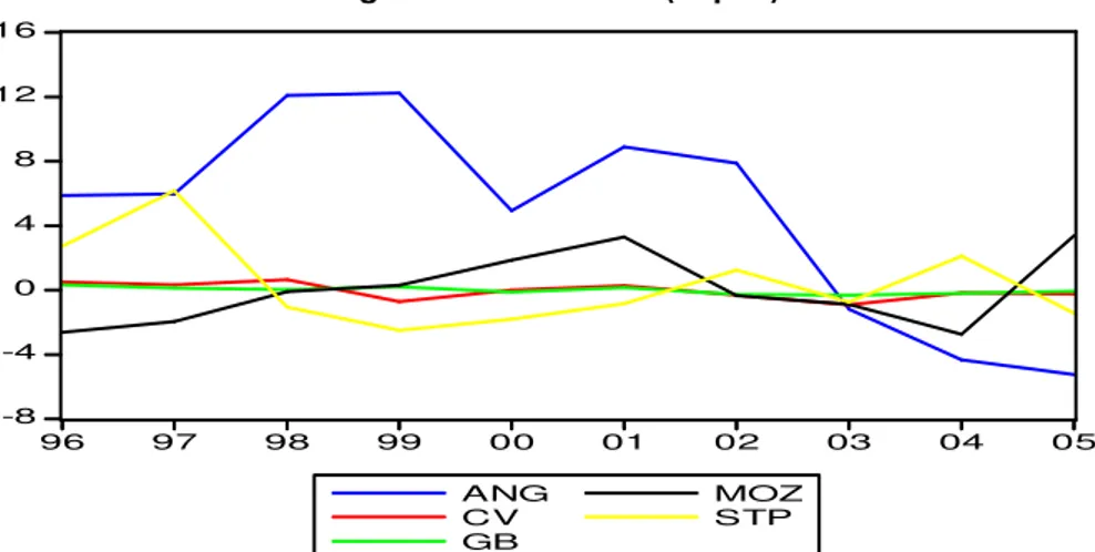
Figure 1 - EMP Mean (% p.a.)
-8 -4 0 4 8 12 16 96 97 98 99 00 01 02 03 04 05 ANG CV GB MOZ STP
Note: Annual values are calculated as average of monthly EMP estimates.
13∆e
t > 0 denote exchange rate depreciations. 14
Recent research highlights that EMP summary statistics calculated using the ERW approach are sensitive to the assumptions regarding their constituent components (see Bertoli, et al., 2006 and also Li et al., 2006). The assumptions of relevance to our analysis have to do with the manner in which exchange rate variations are computed (exact formula versus logarithmic approximation), the different definitions of reserves (gross versus net), the constancy of precision weights over time and the choice of anchor currency. Our robustness analysis indicates that EMP summary statistics obtained under a different set of assumptions are broadly similar to the ones used in the analysis. As such, they will not change the ordinal ranking of PALOP countries’ conditional volatility presented here. The robustness analysis results, which also include estimated precision weights, are available from the authors upon request.
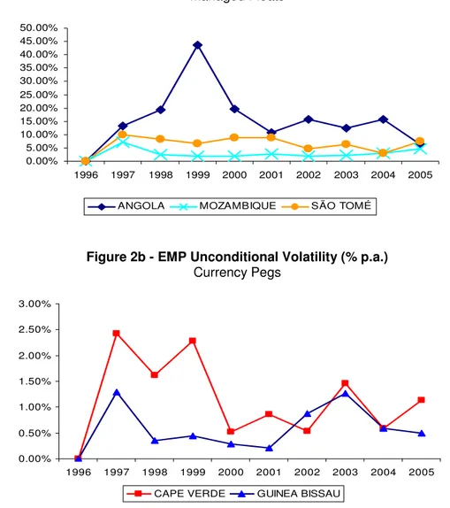
The descriptive statistics of our estimated EMP measures are given in Table 1.15 Looking at mean EMP values, we observe that CV, GB and MOZ are characterised by slightly negative EMP (close to zero) over the sample period, which is of a very similar order of magnitude for all these countries. The other two countries, meanwhile, have positive EMP but the mean for ANG is much larger than that of STP, as is also clear from Figure 1. The unconditional standard deviation and EMP range statistics allows us to refine this observation. Indeed, now we are able to classify the five countries into two distinct groups based on the ranking of these last two descriptive statistics. The countries with currency pegs clearly exhibit lower volatility and a smaller range of EMP variation. The countries with managed floats are much more volatile. ANG exhibits the greatest unconditional volatility (34.87%), followed by STP (7.07%) and then MOZ (4.31%). This classification is confirmed upon inspection of Figure 2, which shows the annual average of monthly EMP standard deviations for the two types of exchange rate arrangements.
Figure 2a - EMP Unconditional Volatility (% p.a.) Managed Floats 0.00% 5.00% 10.00% 15.00% 20.00% 25.00% 30.00% 35.00% 40.00% 45.00% 50.00% 1996 1997 1998 1999 2000 2001 2002 2003 2004 2005
ANGOLA MOZAMBIQUE SÃO TOMÉ
Figure 2b - EMP Unconditional Volatility (% p.a.) Currency Pegs 0.00% 0.50% 1.00% 1.50% 2.00% 2.50% 3.00% 1996 1997 1998 1999 2000 2001 2002 2003 2004 2005
CAPE VERDE GUINEA BISSAU
Next, we proceed to identify crisis episodes, which we take to be those EMP values exceeding some pre-established critical threshold. We bear in mind, however, that the definition of these thresholds entails using a discretional “rule of thumb”. As such, we consider three different thresholds to ensure a more robust analysis. A crisis episode is thus
15
identified when an EMP measure exceeds mean EMP by 1.5 SD, 2.5 SD and 3.5 SD respectively. Accordingly, we classify EMP crises as having a low, moderate or high severity. Note that these classifications will not correspond to the same magnitudes of EMP when comparing across countries, given their different levels of mean EMP. The EMP crises statistics are given in Table 2 while EMP crises tables for each country are provided in the appendix.16
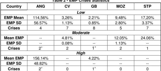
Table 2 - EMP Crises Statistics
Country ANG CV GB MOZ STP
Low EMP Mean 114,56% 3,26% 2.21% 9,48% 17,20% EMP SD 56.57% 1.13% 0.85% 2.80% 3.37% Crises 4 7 8 5 7 Moderate Mean EMP -- 4.81% -- 12.05% 24.06% EMP SD -- 0.08% -- 1.13% -- Crises 2+ 2 1+ 2 1 High Mean EMP 156.14% -- 4.22% -- -- EMP SD 48.82% -- -- -- -- Crises 2+ 0 1+ 0 0
Note: The symbol (+) denotes that the same events are being considered in the calculations.
Our first observation is that the number of crises varies across countries but not significantly. However, the severity of crises differs substantially. In the case of ANG, for example, we identify four crises at the lower threshold of which two are classified as severe. In contrast, GB experienced eight crises but only one of these was a high-severity crisis having a similar order of magnitude as CV’s single moderate-severity crisis. The finding that the severity of crisis differs substantially is reinforced when looking at the average values of EMP during crises episodes. GB and CV had positive EMP crises of magnitude 2.21% and 3.26% respectively at the 1.5SD threshold. The comparable figures for MOZ and STP are 9.48% and 17.20% while that of ANG is 114.56%.
Two findings thus emerge from our crises analysis. First, EMP crises under currency pegs are much less severe than those under managed floats at all threshold levels. Second, ANG has the most severe EMP crises whilst MOZ has the least less severe ones among countries with managed floats. STP, meanwhile, lies between these two extreme but its EMP behaviour is clearly much closer to that of MOZ. We note that these findings corroborate those established in our descriptive analysis above. In order to better understand these findings, we now turn to the study of EMP’s stochastic properties in the next section.
3. EMP Dynamics
Our modelling approach is dictated by two concerns: first, we want to capture possible heteroscedasticity effects, volatility clustering and leverage effects associated with asymmetric responses shocks of the EMP series; second, we want to be able to compare EMP behaviour for the five PALOP countries within an economically meaningful framework. Given these objectives and following the modelling approach adopted in related work (Braga de Macedo et al. (2006), we estimate exponential GARCH in the mean (EGARCH-M) models. These models allow mean EMP to depend on its own conditional variance à la Engle
16 In the tables, crises episodes are identified in bold type while the colours black, blue and red indicate that
et al. (1987), thereby capturing the basic insight that risk-averse agents will require compensation for holding a country’s risky assets, especially as these are typically denominated in domestic currency. Given that an asset’s riskiness can be measured by the variance of returns, the risk premium is an increasing function of the returns’ conditional variance. The actual specification adopted is as follows:
where єt is the error disturbance term, assumed to have a zero mean and to be serially
uncorrelated, and DΘ(0, 1) is a probability density function with zero mean and unit variance.17
The EMP mean equation incorporates the effect of economic fundamentals, whose impact is captured by the k × 1 vector of explanatory variables xt (includes a constant term where
necessary), with θ being the respective 1 × k coefficient vector. The risk-return relationship, meanwhile, is captured by the parameter µ. All explanatory variables are lagged one period in order to avoid the problem of contemporaneous simultaneity with the dependent variable. We also allow for ARMA (m, n) terms given the lack of data pertaining to economic fundamentals for all countries in our sample, as discussed below. In the conditional variance equation, st is an r × 1 vector of explanatory variables (includes a constant term), and λ is the
respective 1 × r coefficient vector. Note that the left-hand side above is the logarithm of the conditional variance, which implies that the associated leverage effect is exponential rather than quadratic. In addition, forecasts of the conditional variance are guaranteed to be non-negative under this specification.
The literature identifies various macroeconomic fundamentals that could be considered as possible explanatory variables in our model. Some of these include:18 a) the rate of inflation, as it is associated with high nominal interest rates and may proxy macroeconomic mismanagement that adversely affects the economy (Demirguc-Kunt & Detragiache, 1997); b) the real exchange rate, given that currency over-valuations may deteriorate the current account and have historically been associated with currency crises (Berg et al., 1999); c) import and export growth which, when problematic, may lead to current account deteriorations that trigger currency crises (Dowling & Zhuang, 2000, Berg & Patillo, 1999); d) growth in monetary aggregates, e.g. excessive M1 growth might indicate excess liquidity and, hence, increased EMP that leads to speculative attacks (Eichengreen et al., 1995); e) domestic credit, given that high debt levels are conducive to banking sector fragility (Kaminsky & Reinhart, 1998); f) public debt, as higher public indebtedness is expected to raise vulnerability to a reversal in capital inflows, and hence to raise the probability of a crisis (Lanoie & Lemarbre, 1996). g) current account, as deficits are associated with large capital inflows, which indicate a diminished probability to devalue and thus lower the probability of a crisis (Berg & Patillo 1999); h) fiscal balance, as deficits are expected to raise the probability
17
Optionally, Θ are additional distributional parameters that can be used to describe a distribution’s skew and shape. For a full discussion of this class of models, refer to Engle (1982) and Bollerslev (1986). In practice, we found that models were best estimated assuming normally-distributed errors.
18
For more details, refer to Feridun (2007), who provides a useful summary that also includes several indicators describing banking sector vulnerability. See also Flood & Marion (1998).
of crisis since they increase the vulnerability to shocks and investor’s confidence (Demirguc-Kunt & Detragiache, 1997).
For PALOP countries, however, our choice of explanatory variables is severely restricted by the lack of data. At best, the publicly available data have a trimesterly or annual frequency, which is too low to use in our econometric models. More frequently, the data simply do not exist. In practice, we are able to use two fundamentals for the mean equation that have the desired monthly frequency (see the appendix for the data description): domestic credit growth rate (dct) and the real depreciation rate (qt).19 In the conditional variance equation, we
include foreign reserve changes (rt) in addition to the afore-mentioned variables, given their
important role in EMP dynamics, especially under currency pegs.20 For ANG, changes in oil prices are also used due to the importance of oil exports in its economy. Explanatory variables are lagged at least one period to avoid possible simultaneity bias in our estimations. The presence of a time trend in our monthly model of EMP is meant to capture the lower frequency trend that may exist in exchange rates due to aggregation of data, in particular, and omitted variables, in general.21
Where appropriate, we test for the inclusion of dummy variables that are related to the occurrence of known economic events, e.g., CV's adoption of a currency peg in 1999:01, GB's implementation of its accession agreement with the WAEMU in 1997:05, etc. (see appendix the for dummy variable definitions). We also consider dummies that capture observed idiosyncratic events which clearly impact our estimations, e.g. the influx of MOZ's donor aid arrears in late 2004 and the subsequent need for depreciation of the MZM in 2005:04/05. In the conditional variance equation, the dummy variables included are identified using Inclan & Tiao's (1994) CSUM test, which tests for structural breaks in volatility.
Turning to the expected signs of the mean equation’s explanatory variables, domestic credit growth necessarily lead to greater EMP, hence estimated coefficients will be positive. On the other hand, real depreciation leads to lower EMP, implying that expected signs are negative. In an EMP context, the risk-return relationship implies that holding assets of a country in which EMP-volatility is high (large σ2
t) should be compensated by a larger return (lower
EMP), implying that µ is negative.22 Note also that µ is interpretable as the semi-elasticity of changes in EMP for a given percentage change in conditional volatility.
As for conditional variance, the expected signs of the explanatory variables are not easily predictable a priori on theoretical grounds but their effects are easily interpretable upon estimation. In the case of foreign reserves, for example, a negative coefficient indicates that an increase in foreign reserves lowers conditional volatility. Finally, the impact of shocks is asymmetric if γ is different form zero while the presence of leverage effects can be tested under the hypothesis that γ is negative, which implies that negative shocks increase volatility more than positive ones of an equal magnitude.23 A plausible explanation for this asymmetric
19
Note that it was not possible to calculate qt for STP due to lack of data regarding prices changes for this
country.
20
Changes in reserves and in the interest rate differential are not included in the mean equation as they are already present in the EMP measure.
21
The first situation may lead to persistence that induces slight regime switching behaviour, due to agents’ perceptions of the market and of policy actions, and possibly by the exchange-rate policy stance.
22
For exchange rates, the risk premium associated with the underlying volatility can be either positive or negative. Engel (1996), for example, shows that the direction of the effect of conditional variance on risk premiums depends on the variance of nominal consumption. Fukuta & Saito (2002), meanwhile, shows that the signs of the coefficients on risk premiums depend on the covariance between consumption growth and inflation, the inter-temporal marginal rate of substitution, and the variances of inflation in Japan and the United States.
23
Standard GARCH models assume that positive and negative error terms have a symmetric effect on the volatility. i.e. good and bad news have the same effect. In practice this assumption is frequently violated, in particular by stock returns, as noted by Black (1976). A likely reason for stock returns' asymmetric leverage effect
leverage effect in the case of EMP is that risk perceptions of negative EMP tend to increase when upside volatility increases more than downside volatility. Moreover, this behaviour is to be expected mainly in mature financial markets, as opposed to those which are less sophisticated and underdeveloped.
Our econometric analysis comprises the relatively short period of 1996:01 to 2005:09, as the adoption of a common analysis period required for cross-country comparisons reduces the effective sample size. In estimating our EGARCH-M models, we started with a general specification of the mean and variance equations. The orders of the variance equation and ARMA process in the mean equation were determined by the partial autocorrelation and the autocorrelation function of the EMP series. Non-significant variables are excluded from estimated equations where appropriate. We use the Schwartz Information Criterion (SIC) to assess a model’s relative fit, implying that we choose those models for which the (negative) SIC is smallest. The final EGARCH-M specifications are decided by looking at the properties of standardised residuals (SR) and squared standardised residuals (SSR).
The models are estimated using E-Views 5.0, and we employ the Marquardt nonlinear optimization algorithm to compute maximum likelihood parameters. Bollerslev & Wooldridge (1992) note that maximising a mis-specified likelihood function in a GARCH framework provides consistent parameter estimates, even though standard errors will be understated. Accordingly, we use their consistent variance-covariance estimator to correct the covariance matrix. As such, we report asymptotic standard errors for estimated parameters which are robust to departures from normality.
Correctly specified EGARCH-M models will have SR and SSR that are white noise, i.e. they are independent and identically distributed random variables with mean zero and variance one. As model diagnostic tools, we use the modified Box-Ljung (B-L) procedure on the SR series to test for remaining serial correlation in the mean equation. To detect remaining ARCH effects in the variance equation, we use the B-L test as well as the ARCH-LM test on SSR. Based on the results of the diagnostic tests, we find ample support for our model specification. The B-L Q-statistics are insignificant at the 5% level for both the mean and variance equation, as are those of the ARCH-LM test.
The summary of our EGARCH-M estimation’s results is given in Table 3.24 For all countries, we find economic fundamentals to be significant in the mean equation, as monetary expansions are associated with higher EMP while real exchange rate depreciations lead to lower EMP. The degree of response appears to differ across countries, however. Our estimations suggest that the effect of a 1% increase in domestic credit on EMP is greatest in CV (5.81%) and MOZ (3.60%, at lag 6).25 This finding apparently suggests that conditions in monetary and exchange rate markets are more closely related in CV and MOZ than in the other countries.
The fact that we do not any find such evidence for GB is probably not unsurprising given the unit of analysis being considered. We are confident that were we to consider changes in domestic credit for whole of the CFA currency area, instead of only those in GB, similar evidence is likely to emerge. For ANG, the apparent weakness of linkages between these markets is reinforced by the fact that estimated coefficients are only significant at the 5% level, which contrasts with the case of other PALOP countries. With regards to real exchange rate depreciations, the evidence is broadly similar across countries with the exception of GB,
is that negative returns imply a larger proportion of debt through a reduced market value of the firm, hence higher volatility.
24Full estimation results and diagnostics are provided in the appendix. 25
A degree of caution must be exercised when interpreting this result, as changes in domestic credit that arise from monetary authorities' sterilisation activities cannot be identified using publicly available data.
where these have a smaller effect on EMP, in all likelihood due to the same reason given above.
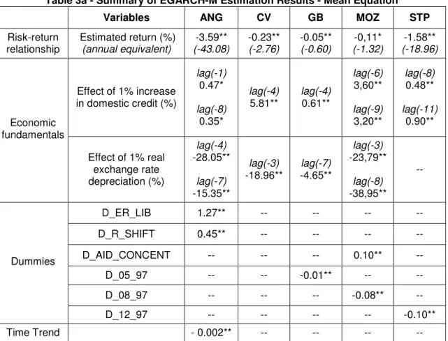
Table 3a - Summary of EGARCH-M Estimation Results - Mean Equation
Variables ANG CV GB MOZ STP
Risk-return
relationship Estimated return (%) (annual equivalent) (-43.08) -3.59** -0.23** (-2.76) -0.05** (-0.60) (-1.32) -0,11* (-18.96) -1.58**
Effect of 1% increase in domestic credit (%) lag(-1) 0.47* lag(-8) 0.35* lag(-4) 5.81** lag(-4) 0.61** lag(-6) 3,60** lag(-9) 3,20** lag(-8) 0.48** lag(-11) 0.90** Economic fundamentals Effect of 1% real exchange rate depreciation (%) lag(-4) -28.05** lag(-7) -15.35** lag(-3) -18.96** -4.65** lag(-7) lag(-3) -23,79** lag(-8) -38,95** -- D_ER_LIB 1.27** -- -- -- -- D_R_SHIFT 0.45** -- -- -- -- D_AID_CONCENT -- -- -- 0.10** -- D_05_97 -- -- -0.01** -- -- D_08_97 -- -- -- -0.08** -- Dummies D_12_97 -- -- -- -- -0.10** Time Trend - 0.002** -- -- -- --
Note: (--) not applicable due to lack of data or relevance. A double (single) asterisk indicates that the estimated parameter is significantly different from zero at the 1% (5%) level.
We also find evidence of the risk-return relationship but it differs across countries rather significantly. While GB has the lowest estimate 0.60% p.a., the estimates CV and MOZ’s estimates are of a close order of magnitude, as a 1% increase in volatility is associated with a reduction in mean EMP of 2.76% and 1.32% p.a. respectively. In contrast, the risk-return relationship in ANG and STP is clearly more extreme, as our estimates imply that holders of these countries assets would respectively expect to be compensated by a 43.08% and a 18.96% p.a. EMP reduction for the same increase in volatility.
The estimates for dummy variables provide additional insight into mean EMP dynamics. The liberalisation of ANG's exchange rate on 2002:12 (dummy D_ER_LIB), possibly coupled with other foreign exchange-market policy management mechanisms introduced around this period, lead to a strong AOA depreciation and significant positive EMP. In addition, during 1999:05, an unexplained and large reduction in ANG’s foreign reserves, which fell from 741.26 to 375.55 million USD, increased EMP (dummy D_R_SHIFT). The same occurs when the MZM depreciates in 2005:04/05 (dummy D_AID_CONCENT), thereby partially reversing the currency’s appreciation streak that resulted from the concentration of donors payment arrears at the end of 2004. GB’s entry to the WAEMU, agreed upon in 1996:12 but only effective as of 1997:05, is clearly associated with a reduction in EMP volatility (dummy D_05_97) and so is MOZ’s substantial reduction in interest rates in 1997:07 (dummy D_8_97). In the case of STP, an inspection of its exchange rate data suggests that some sort of “regime change” takes place toward the end of 1997, which marks the end of period of relatively large STD depreciations (dummy D_12_97). The respective dummy’s estimate
confirms this intuition, as it indicates that this “regime change” effectively lowered EMP as of 1998:01. There is no evidence of time trend behaviour with the exception of ANG, where the estimated coefficient is significant but has a very small magnitude.
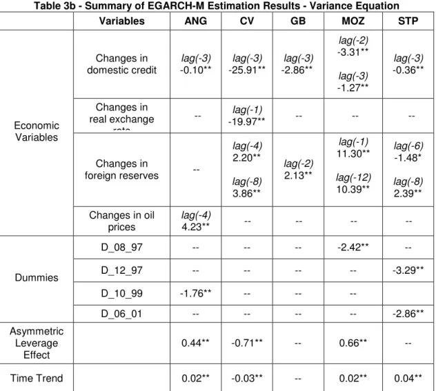
Table 3b - Summary of EGARCH-M Estimation Results - Variance Equation
Variables ANG CV GB MOZ STP
Changes in
domestic credit -0.10** lag(-3) -25.91** lag(-3) -2.86** lag(-3)
lag(-2) -3.31** lag(-3) -1.27** lag(-3) -0.36** Changes in real exchange rate -- -19.97** lag(-1) -- -- -- Changes in foreign reserves -- lag(-4) 2.20** lag(-8) 3.86** lag(-2) 2.13** lag(-1) 11.30** lag(-12) 10.39** lag(-6) -1.48* lag(-8) 2.39** Economic Variables Changes in oil prices lag(-4) 4.23** -- -- -- -- D_08_97 -- -- -- -2.42** -- D_12_97 -- -- -- -- -3.29** D_10_99 -1.76** -- -- -- Dummies D_06_01 -- -- -- -- -2.86** Asymmetric Leverage Effect 0.44** -0.71** -- 0.66** -- Time Trend 0.02** -0.03** -- 0.02** 0.04**
Notes: (--) not applicable due to lack of data or relevance. A double (single) asterisk indicates that the estimated parameter is significantly different from zero at the 1% (5%) level.
Addressing the conditional variance, we find that increases in domestic credit are always associated with lower volatility. This effect seems to be more pronounced in CV, GB and MOZ, as was also the case for mean EMP, and is less pronounced in ANG and STP. Real exchange rate changes have the same effect but only for CV. Foreign reserve changes generally increase volatility with the exception of ANG, where changes oil prices have the same impact.26 Evidence of asymmetric effects of shocks on volatility is found for ANG, CV and MOZ while negative shocks increase volatility more that positive ones only for CV. The absence of the last effect for GB is again probably due to the reason earlier.
Various structural breaks are also found to be associated with lower volatility: 1999:10 (ANG), 1997:08 (MOZ), 1997:12 and 2001:06 (STP). Some of these breaks appear to be associated with known economic events. For instance, the break identified for MOZ in 1997:08 in all likelihood reflects the introduction of the Maputo inter-bank offered rate (MAIBOR) during the previous month, which fell substantially from 35.80% to 13.35%. With the exception of GB, time trend variables are significant for PALOP countries, which
suggests that our model of conditional volatility will benefit from the inclusion of other economic variables should these become available.
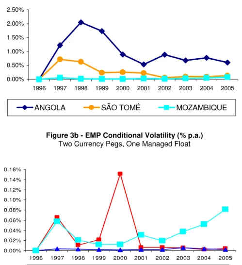
Finally, we look at the conditional volatility series resulting from our model estimations in order to determine whether our initial finding that countries with currency pegs have lower volatility is confirmed. In Figure 3, we again group countries according to their exchange rate regime but now include MOZ in both in order to facilitate comparisons. Overall, we confirm this finding and the ordinal ranking that emerges from observing unconditional volatility (Figure 2). Moreover, two additional observations can be made. First, “pre-peg” CV and MOZ exhibit similar volatility prior to 1999. CV’s currency peg has had markedly lower volatility since then, with the exception of 2000. Since 2002, this difference has been accentuated as MOZ’s volatility has increased further. While the reason for this is unclear, this change might reflect the economic aftermath of the 2000-1 floods that severely affected MOZ. Second, STP’s volatility level has declined since 2002 and is now much closer to that of MOZ, which has the managing float with the lowest conditional volatility.
Figure 3a - EMP Conditional Volatility (% p.a.) Managed Floats 0.00% 0.50% 1.00% 1.50% 2.00% 2.50% 1996 1997 1998 1999 2000 2001 2002 2003 2004 2005
ANGOLA SÃO TOMÉ MOZAMBIQUE
Figure 3b - EMP Conditional Volatility (% p.a.) Two Currency Pegs, One Managed Float
0.00% 0.02% 0.04% 0.06% 0.08% 0.10% 0.12% 0.14% 0.16% 1996 1997 1998 1999 2000 2001 2002 2003 2004 2005
4. Conclusion
Our main conclusion is that PALOP countries with currency pegs clearly have lower volatility when compared to those with managed floats. Moreover, EMP crises under pegs are much less severe. We find that economic fundamentals correctly account for mean EMP for all countries. The response of mean EMP to changes in domestic credit, however, is greatest in CV and MOZ, which apparently suggests that conditions in monetary and exchange rate markets for these countries are closely related. While the evidence is not as strong for GB, this is possibly due to the fact that this country is the only one in our sample which formally belongs to a monetary and currency union having the same legal tender for its members. We also find that the risk-return relationship is much more favourable for investors under currency pegs, as the increase in volatility is lower for the same rate of (EMP) return. The exception to this finding is MOZ, which apparently has a risk-return profile akin to that enjoyed by countries with pegs. A plausible reason is that MOZ has the only managed float in our sample implementing monetary and exchange rate policy within the confines of an IMF framework, which establishes floors for international reserves and ceilings for the central bank’s net domestic assets. This intuition needs to be tested, however, and as such is included in our future research agenda.
EMP conditional volatility, meanwhile, is generally driven by changes in domestic credit (lowers it) and foreign reserve changes (raises it). The first effect is more pronounced under currency pegs, but also under MOZ’s managed float. Evidence of asymmetric effects of shocks on volatility is found for ANG, CV and MOZ while “bad news” increase volatility more that “good news” only for CV’s currency peg, which we take to be a further sign of its credibility.
A few striking cross-country comparisons also emerged in our analysis. We find that ANG has the most severe EMP crises whilst MOZ has the least severe among countries with managed floats. STP, meanwhile, lies between these two extremes but its EMP crises behaviour is clearly much closer to that of MOZ. Our econometric models also permit us to rank PALOP countries’ conditional volatility in ordinal terms. Based on these findings, it appears that MOZ’s managed float has the greatest credibility for such arrangements as it has lowest volatility while ANG has the highest. STP’s credibility may also be improving since its volatility has declined as of 2002 and its level is now much closer to that of MOZ.
Our future research agenda seeks to refine the above insights by seeking more data and better institutional knowledge for PALOP countries. This will allow us, for example, to fully explore crises episodes and structural breaks, and then relate these to policy and institutional changes. We also plan to undertake a comparative analysis using multivariate techniques, which might be instructive in terms of better policy design in the future. Hopefully, the techniques developed for this undertaking will also allow us to investigate other cases of interest in Africa, such as the CFA arrangement and the South African Rand’s monetary zone.
References
Andreou, E. and E. Ghysels (2002) “Detecting Multiple Breaks in Financial Market Volatility Dynamics”, available at http://ssrn.com/abstract=313639.
Berg, A., and C. Pattillo (1999) “Predicting Currency Crises: the Indicators Approach and an Alternative”, Journal of International Money and Finance, Vol. 18, No. 4, (August), pp. 561-586. Bertoli, S., Gallo G. M. and G. Ricchiuti (2006) “Exchange Market Pressure: Some Caveats in Empirical Applications”, Working Paper 2006/17, Department of Statistics, University of Florence, Italy. Black, F. (1976) “Studies in Stock Price Volatility Changes”, Proceedings of the 1976 Meeting of the
Business and Economic Statistics Section, American Statistical Association, pp. 177-181.
Bollerslev, T. (1986) “Generalized Autoregressive Conditional Heteroscedasticity”, Journal of
Econometrics, No. 31, pp. 307-27.
Bollerslev, T. and J. Wooldridge (1992) “Quasi-Maximum Likelihood Estimation and Inference in Dynamic Models with Time Varying Covariances”, Econometric Reviews, No. 11, pp. 143-172.
Bonaglia, F., Braga de Macedo, J. and M. Bussolo (2001) “How Globalisation Improves Governance”, CEPR Discussion Paper, No. 2992, October.
Braga de Macedo, J., Eichengreen B. and J. Reis (1996) editors, Currency Convertibility: The Gold
Standard and Beyond, London: Routledge.
Braga de Macedo, J. (2001a) “Crises? What Crises? Escudo from ECU to EMU”, in Short-Term
Capital Flows and Economic Crises, edited by Stephany Griffith-Jones, Manuel Montes and Anwar
Nasution, study prepared for UNU/WIDER, Oxford University Press, pp.253-260.
Braga de Macedo, J., Cohen, D. and H. Reisen (2001b), editors, Don’t Fix Don’t Float, Paris: OECD Development Centre.
Braga de Macedo, J. and B. Eichengreen (2001c) “The European Payments Union and its Implications for the Evolution of the International Financial Architecture”, in Fragility of the International Financial
System - How Can We Prevent New Crises in Emerging Markets?, edited by Alexandre Lamfalussy,
Bernard Snoy and Jérôme Wilson, Brussels: PIE Peter Lang for Fondation Internationale Robert Triffin, pp. 25-42.
Braga de Macedo, J., Nunes, L. C. and L. Brites Pereira (2003) “Central Bank Intervention Under Target Zones: The Portuguese Escudo in the ERM”, FEUNL Working Paper, No. 345, Lisbon: Universidade Nova de Lisboa.
Braga de Macedo, J., Catela Nunes, L. and F. Covas (2004a) “Moving the Escudo into the Euro” in chapter 8 of Shaping the New Europe: Economic Policy Challenges of EU Enlargement, edited by Michael Landersmann and Darius Rosati, Palgrave, forthcoming (an earlier version appeared as CEPR Discussion Paper, No. 2248, October 1999).
Braga de Macedo, J. and H. Reisen (2004b), “Float in Order to Fix: Lessons from Emerging Markets for New EU Member Countries”, in Monetary Strategies for Joining the Euro, National Bank of Hungary, pp. 109-113.
Braga de Macedo, J. and M. Grandes (2005) “Argentina and Brazil Risk: a Eurocentric Tale”, in Rolf Langhammer e Lucio Vinhas de Souza, editors Monetary Policy and Macroeconomic Stabilization in
Latin America, Berlin: Springer, pp. 153-172.
Braga de Macedo, J., Braz, J., Brites Pereira, L. and L. C. Nunes (2006) Report to the Monetary Authority of Macau on “Macau’s Currency Board”, FEUNL Working Paper No. 492, Lisbon: Universidade Nova de Lisboa.
Braga de Macedo, J. and J. Oliveira Martins (2006) “Growth, Reform Indicators and Policy Complementaries, FEUNL Working Paper No. 484, Lisbon: Universidade Nova de Lisboa.
Braga de Macedo, J. & L. Brites Pereira, (2006) “The Credibility of Cape Verde’s Currency Peg”, FEUNL Working Paper No. 494, Lisbon: Universidade Nova de Lisboa.
Brites Pereira (2005a), “The Effectiveness of Intervention: Evidence from a Markov-Switching Analysis”, Manuscript, Doctoral Thesis, Lisbon: Universidade Nova de Lisboa.
Brites Pereira (2005b), “Relieving Exchange Market Pressure”, Manuscript, Doctoral Thesis, Lisbon: Universidade Nova de Lisboa.
Bubula, A. and I. Otker-Robe (2006) “Are Pegged and Intermediate Exchange Rate Regimes More Crisis Prone?, IMF Working Paper No. 03/223, Washington: International Monetary Fund.
Collier, P. (2006) “Angola: Options for Prosperity”, Department of Economics, Oxford University, available at users.ox.ac.uk/~econpco/research/Africa.htm.
Demirguc-Kunt, A. and E. Detragiachhe (1997) “The Determinants of Banking Crises in Developing and Developed Countries”, IMF Working Paper No. 106, Washington: International Monetary Fund, pp. 34-56.
Dooley, M. Folkerts-Landau, D. and P. Garber (2005) “Interest rates, Exchange Rates and International Adjustment”, NBER Working Paper, No. 11771.
Dowling, M. and J. Zhuang (2000) “Causes of the 1997 Asian financial crisis: What More Can We Learn from an Early Warning System Model?”, Department of Economics, Melbourne University, Australia Working Paper No. 123, pp. 54-76.
Engel, C., (1996), “The Forward Discount Anomaly and the Risk Premium: A Survey of Recent Evidence”, Journal of Empirical Finance, No. 3, pp.123-192.
Engle, R. (1982) “Autoregressive Conditional Heteroscedasticity with Estimates of the Variance of United Kingdom Inflation”, Econometrica, No. 50, pp. 987-1007.
Engle, R., Lilien, D. and R. Robins (1987) “Estimating Time Varying Risk Premia in the Term Structure: The ARCH-M Model”, Econometrica, No. 55, pp. 391-407.
Eichengreen, B., Tobin, J. and C. Wyplosz (1995) “Two Cases for Sand in the Wheels of International Finance”, Economic Journal, Vol. 105, pp. 162-172.
Eichengreen, B., Rose, A. K. and C. Wyplosz (1995) “Exchange Market Mayhem: The Antecedents and Aftermath of Speculative Attacks”, Economic Policy,Vol. 21, pp. 249-312.
Eichengreen, B., Rose, A. K. and C. Wyplosz (1996) “Speculative Attacks on Pegged Exchange Rates: An Empirical Exploration with Special Reference to the European Monetary System”, in Canzoneri, M.B., Ethier W.J. and V. Grilli (eds.) The New Transatlantic Economy, Cambridge University Press, Cambridge.
Feridun, M. (2007) “An Econometric Analysis of the Mexican Peso Crisis of 1994-1995”, Doğuş
Üniversitesi Dergisi, No. 8 (1), pp. 28-35.
Flood, R. and N. Marion (1998) “Perspectives on Recent Currency Crisis Literature”, NBER Working Paper No. 6380, Cambridge, MA: National Bureau of Economic Research.
Fukuta, Y. and M. Saito (2002) “Forward Discount Puzzle and Liquidity Effects: Some Evidence from Exchange Rates among the United States, Canada, and Japan”, Journal of Money, Credit and
Girton, L. and D. Roper (1977) “A Monetary Model of Exchange Market Pressure Applied to the Postwar Canadian Experience”, American Economic Review, Vol. 67, No. 4, pp. 537-48.
Goldberg, L. and M. Klein (2006) “Establishing Credibility: Evolving Perceptions of the European Central Bank”, paper presented at the NBER Summer Institute, July.
Inclán, C. and C. Tiao (1994) “Use of Cumulative Sums of Squares for Retrospective Detection of Changes of Variance”, Journal of the American Statistics Association, Vol. 89, pp. 913-23.
Kaminsky, G.L. and C.M. Reinhart, (1999) “The Twin Crises: The Causes of Banking and Balance of Payments Problems”, American Economic Review, Vol. 89 (June), pp. 473-500.
Kim, K. and P. Schmidt (1993) “Unit root tests with Conditional heteroskedasticity”, Journal of
Econometrics 59, 287-300.
Kose, M., Prasad, E., Wei, S. and K. Rogoff (2006) “Financial Globalization: A Reappraisal”, IMF Working Paper No. 06/189, Washington: International Monetary Fund.
Kouri, P. and J. Braga de Macedo (1978) “Exchange Rates and the International Adjustment Process”, Brookings Papers on Economic Activity.
Krugman, P. (1981) “Oil and the Dollar”, in J. Bhandari and J. Putnam, Interdependence under
Flexible Exchange Rates, Cambridge: MIT Schuler, K. (2004) Tables of Modern Monetary History, available at http://users.erols.com/kurrency/afrca.htm
Lanoie, P. and S. Lemarbre (1996) “Three Approaches to Predict the Timing and Quantity of LDC Debt Rescheduling”, Applied Economics, No. 28 (2), pp. 241-246.
Li, J. Rajan, R.S and T. Willett (2006) Measuring Currency Crises using Exchange Market Pressure Indices: the Imprecision of Precision Weights, available at www.princeton.edu/~pcglobal/conferences/IPES/papers/chiu_willett_S1100_1.pdf
Spolander, M. (1999) “Measuring Exchange Rate Pressure and Central Bank Intervention”, Bank of
Finland Studies, Series E, No. 17.
Veyrune, R. (2007) “Fixed Exchange Rate and the Autonomy of Monetary Policy: The Franc Zone Case”, IMF Working Paper, No. 07/34
Weber, R. (2005) “Cape Verde’s Exchange Rate Policy and its Alternatives”, BCL Working Paper No. 16, Banque Central du Luxembourg.
Weymark, D. N. (1995) “Estimating Exchange Market Pressure and the Degree of Exchange Market Intervention for Canada”, Journal of International Economics, Vol. 39, pp. 273-295.
Weymark, D. N. (1998) “A General Approach to Measuring Exchange Market Pressure”, Oxford
APPENDIX – Country Files
ANG – EMP Constituent Components
0 10 20 30 40 50 60 70 80 90 96 97 98 99 00 01 02 03 04 05
AOA/USD Exchange Rate
-0.4 0.0 0.4 0.8 1.2 1.6 96 97 98 99 00 01 02 03 04 05
% Exchange Rate Change
0 500 1000 1500 2000 2500 3000 96 97 98 99 00 01 02 03 04 05
Foreign Reserves (million USD)
-1.2 -0.8 -0.4 0.0 0.4 0.8 1.2 96 97 98 99 00 01 02 03 04 05
% Foreign Reserves Change
-50 0 50 100 150 200 250 300 96 97 98 99 00 01 02 03 04 05
Interest Rate Differential (%)
-280 -240 -200 -160 -120 -80 -40 0 40 96 97 98 99 00 01 02 03 04 05
% Interest Differential Change
ANG – EMP and Changes in Exchange Rate (%)
-300 -200 -100 0 100 200 96 97 98 99 00 01 02 03 04 05
ANG – EMP Estimates & Crises
ANG – EMP Descriptive Statistics
0 10 20 30 40 50 60 -200 -100 0 100 200 Series: EMP_USD Sample 1996M01 2005M09 Observations 117 Mean 5.063191 Median 4.291403 Maximum 190.6627 Minimum -210.6031 Std. Dev. 34.82329 Skewness -0.376357 Kurtosis 21.51951 Jarque-Bera 1674.751 Probability 0.000000
ANG – EGARCH-M Estimation Results 2 3 3 2 2 5 7 4 4 3 8 2 1 2 Dummies ln 1 t− t− + t− + t− + + 1 t− t− + t+ t−
t=µ σ + +θ∆dc +θ ∆dc θq θq θtrend ξEMP +ξ EMP ε ξε
EMP
Parameter Estimate Std. Error t-Statistic p-value
µ -0.035880 0.005544 -6.471381 0.0000** D_ER_LIB 1.266598 0.093339 13.56991 0.0000** D_R_SHIFT 0.450566 0.017936 25.12039 0.0000** 1
θ
0.004743 0.002137 2.219570 0.0264* 2θ
0.003540 0.001580 2.241065 0.0250* 3 θ -0.280504 0.081915 -3.424354 0.0006** 4 θ -0.153451 0.056601 -2.711125 0.0067** 5 θ -0.001997 0.000353 -5.663922 0.0000** 1ξ
-0.621861 0.096220 -6.462932 0.0000** 2ξ
-0.171173 0.045946 -3.725557 0.0002** 2 − t ε 0.756265 0.090967 8.313628 0.0000** 1 1 2 1 2 1 1 4 3 2 DUMMY ln ln − − − − − − − + + + t t 1 t t t 1 t 2 t 1 0 t σ ε γ + σ α σ ε α ∆oil λ + ∆dc λ + λ = σ D_10_99 -1.776190 0.435467 -4.078814 0.0000** λ0 -6.140849 0.417547 -14.70697 0.0000** λ1 4.232692 1.351095 3.132786 0.0017** λ2 -0.095852 0.020470 -4.682682 0.0000** 1 2 lnσ t− -0.634700 0.097083 -6.537693 0.0000** α1 0.320883 0.148388 2.162460 0.0306* γ1 0.442317 0.090149 4.906518 0.0000** DiagnosticsL-B Standardised Residuals L-B Squared Residuals ARCH-LM Statistic
Lag Q p-value Q2 p-value LM p-value
Lag4 2.0716 0.150 1.8103 0.178 0.135892 0.2705 Lag5 2.0751 0.354 1.8394 0.399 0.000934 0.9926 Lag6 2.3794 0.497 1.9752 0.578 -0.024754 0.7787 Lag7 2.8713 0.580 2.0955 0.718 -0.055129 0.6503 Lag8 7.1675 0.208 3.3038 0.653 0.027496 0.8028 Lag9 8.8914 0.180 3.3038 0.770 0.019331 0.8729 Lag10 11.338 0.125 3.3226 0.854 -0.026169 0.8375 Lag11 11.346 0.183 3.6091 0.891 0.043421 0.7131 Lag12 11.360 0.252 4.3461 0.887 0.066988 0.5932 Lag13 11.773 0.301 5.2516 0.874 -0.156820 0.0759 Lag14 13.228 0.279 7.2139 0.782 -0.143736 0.1594 Lag15 13.336 0.345 7.9415 0.790 -0.025106 0.8390
No. of Observations Log-Likelihood SIC
ANG – Data Description27 Variables
et Bilateral AOA/USD exchange rate. Source: IMF – International Financial Statistics
∆et Depreciation rate of AOA vis-à-vis the USD (log).
∆rt Change in ANG’s international reserves (log). Source: IMF – International Financial Statistics. it ANG 3-Month Deposit Rate (%). Source: IMF – International Financial Statistics. it*
USA 3-Month CDs (secondary market), an average of dealer bid rates on nationally traded certificates of deposit (%).
Source: US Federal Reserve.
∆(it - it*) Change in interest rate differential (%).
pt ANG Consumer Price Index. Source: IMF – International Financial Statistics.
∆pt ∆pt = (pt - pt-1)/pt-1 pt*
US Consumer Price Index.
Source: Bureau of Labour Statistics - All Urban Consumers - (CPI-U) U.S. city average. All items 1982-84=100.
∆pt* ∆pt* = (pt* - pt-1*)/pt-1*
q t Real exchange rate depreciation = ∆e - ∆pt + ∆pt* dc t Domestic credit growth rate. Source: IMF – International Financial Statistics.
∆dc t ∆dc t = (dc t - dc t -1)/dc t -1 oil t
Crude Oil (Petroleum), Simple Average Of Three Spot Prices; Dated Brent, West Tx Intermediate, & The Dubai Fateh, USD per Barrel – World.
Source: Wood Mackenzie. ∆oil t ∆oil t = (oil t - oil t-1)/oil t-1
D_10_99 Dummy variable that takes on value one for all t ≥ 1999:10 and zero otherwise.
ER_LIB Dummy variable that takes on value one for all t = 1999:05 and zero otherwise.
D_ER_SHIFT Dummy variable that takes on value one for all t = 2002:12 and zero otherwise.
Unit Root Test: MacKinnon Critical Values Significance Level No Intercept or Trend Intercept Intercept and Trend 1% -2.5830 -3.4861 -4.0373 5% -1.9426 -2.8857 -3.4478 10% -1.6171 -2.5795 -3.1488 27
The data used in the analysis are monthly and the sample period runs from 1996:01 until 2005:09. Where appropriate, ∆ denotes percentage changes between two consecutive months, which are calculated using the exact formula or log difference approximation (excepting interest rate data).
ANG – Phillips-Perron Test Statistic
Series Level Test
Specification
First
Difference Test Specification
pt -1.219924 Intercept & Trend -4.870490** Intercept & Trend pt* -0.382614 Intercept & Trend -4.732785** No Intercept or Trend
et -2.456632 Intercept & Trend -8.137548** No Intercept or Trend it-it* -3.757466** Intercept & Trend -10.97336** No Intercept or Trend rt -0.731256 Intercept & Trend -11.03994** No Intercept or Trend dct -2.032350 Intercept & Trend -11.61337** No Intercept or Trend oilt -0.252769 Intercept & Trend -10.25041** No Intercept or Trend
Notes: The Phillips-Perron procedure tests the null hypothesis of a unit root. All tests were conducted using four lags. A double (single) asterisk indicates that the test statistic is significant at the 1% (5%) level. ANG -30 -20 -10 0 10 20 30 96 97 98 99 00 01 02 03 04 05 % Domestic Credit Change
ANG -.3 -.2 -.1 .0 .1 .2 .3 96 97 98 99 00 01 02 03 04 05 % Oil Price Change
ANG – Country Overview28
Angola’s monetary authority is the Banco Nacional de Angola (BNA, National Bank of Angola in English) and the national currency is the Kwanza (AOA). From the BNA’s webpage the exchange rate on 21.8.07 was of 74.784 AOA/USD according to the available information on the Central Bank. The Kwanza was introduced after the independence of ANG from Portugal substituting the Angolan Escudo entering circulation on the 8th of January 1977, even though the emission date of some of the currency was 1976. On the 25th of September 1990 the New Kwanza (AON) was introduced, then on 1st of July 1995 the readjusted Kwanza (AOR) and on the 1st of December 1999 the Kwanza (AOA) as we know it.
In March 1999 the government started implementing a programme to ensure conditions for economic development and mitigate the negative impact of resumption of the domestic conflict from 1998-1999. Therefore, since May 1999 the BNA, has floated the kwanza, created an interbank foreign exchange market, liberalized foreign exchange purchase for imports as well as established commercial banks interest rates, and to allow for indirect monetary control, created central bank bills. Several steps towards opening the economy were made such as reducing the level and number of import tariff rates and domestic subsidies on fuel prices were eliminated. According to the IMF’s (PIN) No. 05/85 July 6, 2005, on September 2003 the authorities started implementing what is known as the strong kwanza policy and in order to implement this policy, according to the before quoted source, absorption of domestic liquidity was performed through central banks sales of foreign reserves, tightening in the monetary policy along with improvements in fiscal control and domestic debt sales. Altogether it resulted in a considerable reserves shortfall that soon recovered by 2004 and 2005. In fact it is visible on the series that starting on September 2003, for 3 consecutive months the Kwanza appreciates and from December onwards the fluctuation was considerably lower than before this policy shift.
ANG had a GDP of 13.825 million USD in 2003 and 838 USD per capita according to the Public Information Notice (PIN) No. 05/85, July 6. Following on the World Bank’s (WB) country brief August 2007, 12 month inflation was of 12.2% in December 2006, when according to the IMF 10% was targeted. The country has been struggling to contain inflation, in 1998 the country had 135% and reached 330% in 1999 (IMF’s (PIN) No. 00/62, August 10) due to increase of hostilities in 1998 and 1999. The authorities endured in a Staff Monitored Programme (SMP) from April – December 2000 and by June 2001 inflation was of 175% even though 150% was programmed on a January-June 2001 SMP based on the Preliminary Conclusions of the IMF Mission, August 14, 2001. This divergence was a result of excessive foreign borrowing and public spending. However after the peace process of 2002, inflation fell from 106% to 31% in 2004, reaching 12.2% in 2006. The strong export performance along with the strong kwanza policy set the ground for the inflation reduction.
On April the 4th of 2002, the Angolan armed forces and the National Union for the Total Independence of Angola (UNITA) signed an agreement to end the 27-year long civil war. The months that followed witnessed a rapid demobilization and the beginning of the resettlement of ex-combatants across the country, in the context of a government-led initiative that was supported by various UN agencies and the World Bank. The country in general, and especially the government are very dependent on oil revenue whether we speak of foreign
28Information Source: Public Information Notice No. 05/85 - July 6, 2005; No. 03/114 - September 10, 2003; No.
00/62 - August 10, 2000.
Angola -2007 Article IV Consultation Preliminary Conclusions of the Mission, Luanda June 6, 2007 Angola -006 Article IV Consultations - Preliminary Conclusions of the IMF Mission - March 29, 2006 Angola - 2002 Article IV Consultation - Preliminary Conclusions of the IMF mission – Feb. 19, 2002 Angola - Article IV Consultation - Preliminary Conclusions of the IMF Mission August 14, 2001 Angola - Memorandum of Economic and Financial Policies - April 3, 2000