Robust Controller Design for an Autonomous Underwater Vehicle

(1)

UNIVERSIDADE DA BEIRA INTERIOR

Engenharia

Robust Controller Design for an Autonomous

Underwater Vehicle

Carlos Hugo Ribeiro Mendes

Dissertação para obtenção do Grau de Mestre em

Engenharia Aeronáutica

(Ciclo de estudos integrado)

Orientador: Prof. Doutor Kouamana Bousson

(2)

(3)

Dedication

To my parents for all the support and dedication.

”A dream is your creative vision for your life in the future. You must break out of your current comfort zone and become comfortable with the unfamiliar and the unknown.”

(4)

(5)

Acknowledgments

First and foremost, I would like to thank my supervisor, Professor Kouamana Bousson, for pro-viding me guidance and support throughout this work.

I would like to express my deep gratitude to both of my co-supervisors, Tiago Rebelo and Cris-tiano Bentes, and all the engineers at CEiiA, who provided outstanding support during my In-ternship at CEiiA.

My special thanks to my parents, Carlos and Maria, to my brothers, Cátia and Pedro, and to my girlfriend, Mafalda, for the unconditional love, patience and support.

(6)

(7)

Resumo

É visível, a nível mundial, um aumento considerável do interesse em Veículos Autónomos Sub-aquáticos (Autonomous Underwater Vehicles - AUV). O que torna esta tecnologia tão atraente é a capacidade de operar sem intervenção humana. Contudo, a ausência do ser humano restringe a operação do AUV ao seu sistema de controlo, computação e capacidades de detecção. Desta forma, conceber um controlo robusto é obrigatório para viabilizar o AUV.

Motivado por este facto, esta tese tem como objetivo apresentar, discutir e avaliar duas soluções de controlo linear, a propor a um AUV desenvolvido por um consórcio liderado pelo CEiiA. Para que o projeto do controlador seja possível, o modelo dinâmico deste veículo e respectivas con-siderações são primeiramente abordados.

Com a finalidade de possibilitar a operação do veículo, torna-se essencial a elaboração de leis de guidance adequadas. Para este efeito são apresentados algorítmos de Waypoint following e Station keeping, e de path following.

Para a projeção dos controladores é derivada uma versão linear do modelo dinâmico, con-siderando um único ponto operacional. Através da separação do modelo linear em três sub-sistemas são criados quatro controladores Proporcional Integral Derivativo (PID) para cada grau de liberdade (Degree Of Freedom - DOF) do veículo. É também projetado um Regulador Linear Quadrático (LQR), baseado na separação do modelo linear em dois subsistemas, longitudinal e lateral. É ainda apresentada uma lei de alocação de controlo para distribuir o sinal de saída dos controladores pelos diferentes atuadores. Esta provou melhorar a manobrabilidade do veículo. Os resultados finais apresentam um desempenho sólido para ambos os métodos de controlo. No entanto, neste trabalho, o LQR provou ser mais rápido do que o PID.

Palavras-chave

Veículo Autónomo Subaquático; Controlo Robusto; Proportional Integral Derivativo (PID); Regu-lador Linear Quadrático (LQR); Simulação.

(8)

(9)

Abstract

Worldwide there has been a surge of interest in Autonomous Underwater Vehicles (AUV). The ability to operate without human intervention is what makes this technology so appealing. On the other hand, the absence of the human narrows the AUV operation to its control system, computing, and sensing capabilities. Therefore, devising a robust control is mandatory to allow the feasibility of the AUV.

Motivated by this fact, this thesis aims to present, discuss and evaluate two linear control solu-tions being proposed for an AUV developed by a consortium led by CEiiA. To allow the controller design, the dynamic model of this vehicle and respective considerations are firstly addressed. Since the purpose is to enable the vehicle’s operation, devising suitable guidance laws becomes essential. A simple waypoint following and station keeping algorithm, and a path following al-gorithms are presented.

To devise the controllers, a linear version of the dynamic model is derived considering a sin-gle operational point. Then, through the decoupling of the linear system into three lightly interactive subsystems, four Proportional Integral Derivative controllers (PIDs) are devised for each Degree Of Freedom (DOF) of the vehicle. A Linear Quadratic Regulator (LQR) design, based on the decoupling of the linear model into longitudinal and lateral subsystems is also devised. To allocate the controller output throughout the actuators, a control allocation law is devised, which improves maneuverability of the vehicle. The results present a solid performance for both control methods, however, in this work, LQR proved to be slightly faster than PID.

Keywords

Autonomous Underwater Vehicle; Robust Control; Proportional Derivative Integral Derivative (PID); Linear Quadratic Regulator (LQR); Simulation.

(10)

(11)

4.3 PID control . . . 50 4.3.1 Speed Controller . . . 50 4.3.2 Heading Controller . . . 51 4.3.3 Depth Controller . . . 53 4.3.4 Simulink Representation . . . 56 4.4 LQR control . . . 57 4.4.1 Longitudinal Controller . . . 57 4.4.2 Lateral Controller . . . 62 4.4.3 Simulink Representation . . . 63 4.5 Control Allocation . . . 64 4.6 Control Considerations . . . 64

5 Computational Simulation and Validation 65 5.1 Considerations about the Simulations . . . 66

5.1.1 State Feedback . . . 66

5.1.2 Thrust Output . . . 66

5.1.3 Simulation Parameters . . . 66

5.1.4 Ocean Currents . . . 66

5.2 Waypoint following simulation . . . 66

5.2.1 Two-dimensional simulation . . . 66

5.2.2 Three-dimensional simulation . . . 69

5.3 Path following simulation . . . 71

6 Conclusions and Future Work 75 6.1 Concluding Remarks . . . 76

6.2 Future Work . . . 76

Bibliography 77 A Datasheet 81 B Simulations Graphics 83 B.1 Three-dimensional Waypoint Following . . . 83

(13)

List of Figures

1.1 Underwater Vehicle class division. . . 1

1.2 SQX-500 AUV (left) and Girona 500 AUV (right). . . 2

1.3 Seabed AUV. . . 2

1.4 3D model of the developed AUV at CEiiA (courtesy of CEiiA). . . 3

1.5 Ascent and descend scenario (courtesy of CEiiA). . . 4

1.6 Resource exploration and mapping (courtesy of CEiiA). . . 5

1.7 High resolution habitat mapping (courtesy of CEiiA). . . 5

1.8 Body-fixed and local NED reference frames. . . 6

1.9 GNC signal flow diagram. . . 11

1.10 Motion control hierarchy. . . 14

1.11 Block diagram of a generic architecture of a open-loop system. . . 15

1.12 Block diagram of a generic architecture of a closed-loop system. . . 15

1.13 Feedback system block diagram. . . 15

1.14 Feedback block diagram with PID controller. . . 16

1.15 Action of a PID controller. . . 17

1.16 Wind-up effect. . . 18

1.17 Controller with back-calculation loop. . . 18

1.18 Linear quadratic regulator system. . . 19

1.19 Stability in the complex plane. . . 22

1.20 Closed loop system subjected to external disturbances. . . 25

1.21 AUV’s fields of study. . . 26

2.1 General dimensions of the AUV (not to scale). . . 29

3.1 Line Of Sight guidance in the steering plane. . . 37

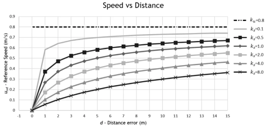
3.2 Influence of the parameter ksin the reference speed. . . 38

3.3 Mode weight funtion: ucmS=udmS=0.5 m/s; ucmI=udmI=0.3 m/s and σcm∗ =σ∗dm=0.05. 39 3.4 Waypoint follower and position holder fluxogram. . . 41

3.5 Path following scheme. . . 43

3.6 Path following fluxogram. . . 44

3.7 Waypoint follower and position holder diagram. . . 45

3.8 Illustration of the waypoint following scenario in the presence of ocean currents. 46 4.1 PID design process. . . 50

4.2 Open- and closed-loop Bode plot of PID speed controller. . . 51

4.3 PID speed controller simulation. . . 51

4.4 Open- and closed-loop Bode plot of PD heading controller. . . 53

4.5 PD heading controller simulation. . . 53

4.6 Open- and closed-loop Bode plot of PID heave controller. . . 54

4.7 PID heave controller simulation. . . 55

4.8 Open- and closed-loop Bode plot for the PID pitch controller. . . 55

4.9 PID pitch controller simulation. . . 56

4.10 Simulink implementation of PID control. . . 56

(14)

4.12 Influence of Ktrgin gain ϕz. . . 60

4.13 LQR speed controller tracking a reference over time. . . 61

4.14 LQR heave controller tracking a reference over time. . . 61

4.15 LQR pitch controller tracking a reference over time. . . 61

4.16 LQR lateral controller simulation. . . 63

4.17 Simulink implementation of LQR control. . . 63

5.1 PID tracking results for two-dimensional simulation. . . 67

5.2 PID evolution of the vehicle’s position in North vs East plot for the two-dimensional simulation. . . 67

5.3 LQR tracking results for two-dimensional simulation. . . 68

5.4 LQR evolution of the vehicle’s position in North vs East plot for the two-dimensional simulation. . . 68

5.5 Roll angle for two-dimensional simulation. . . 69

5.6 PID tracking results for three-dimensional simulation. . . 69

5.7 LQR tracking results for three-dimensional simulation. . . 70

5.8 LQR and PID results of three dimensional waypoint following scenario. . . 70

5.9 LQR and PID simulation of the vehicle’s position in North vs East plot for the path following scenario without beginning constrain. . . 71

5.10 LQR and PID three-dimensional results for path following scenario, without begin-ning constrain (color bar indicates total velocity). . . 72

5.11 LQR and PID simulation of the vehicle’s position in North vs East plot for the path following scenario, with beginning constrain. . . 72

5.12 LQR and PID three-dimensiona results for path following scenario, with beginning constrain (color bar indicates total velocity). . . 73

A.1 Datasheet of the Argus Ars 800 mini thruster. . . 81

B.1 Three-dimensional waypoint following simulation of the PID controller (color bar indicates velocity). . . 83

B.2 Three-dimensional waypoint following simulation of the LQR controller (color bar indicates total velocity). . . 83

(15)

List of Acronyms

AOSN Autonomous Oceanographic Sampling System AUV Autonomous Underwater Vehicle

CEiiA Centre of Engineering and Product Development CFD Computational Fluid Dynamics

COA Circle Of Acceptance DOF Degree-of-Freedom DSV Deep Submersible Vehicle DVL Doppler Velocity Log

EMEPC Estrutura de Missão para a Extensão da Plataforma Continental GNC Guidance, Navigation and Control

HOSM High Order Sliding Mode INS Inertial Navigation System IMU inertial measurement units LHP Left Half Plane

LOS Line Of Sight

LQG Linear Quadratic Gaussian LQR Linear Quadratic Regulator LOS Line Of Sight

LTI Linear Time Invariant

MIMO Multiple Input Multiple Output NED North-East-Down

NN Neural Networks

ODEs ordinary differential Equations PID Proportional Integral Derivative POC Proof Of Concepts

RHP Right Half Plane

ROV Remotely Operated Vehicle SISO Single Input Single Output

SNAME Society of Naval Architects and Marine Engineers SMC Sliding Mode Control

SPURV Self-Propelled Underwater Research Vehicle TTT Time To Targe

UBI University of Beira Interior UUV Unmanned Underwater Vehicle

(16)

(17)

Nomenclature

0b Origin of the body-fixed frame 0n Origin of the inertial frame

{b} Body frame

{n} Inertial frame

AL Longitudinal system matrix

ALa Longitudinal system matrix with integral states

AH Lateral system matrix

B Buoyancy force

BH Input Lateral matrix BL Input Longitudinal matrix

BLa Input Longitudinal matrix with integral states

CA Coriolis and centripetal effects due to added mass CRB Coriolis and centripetal forces acting on the rigid body D Hydrodynamic damping matrix

dk Planar (xy) distance to the waypoint

du Complementary planar distance (xy) to the waypoint ez Depth error

fb

B Buoyancy force vector in the body fixed frame fn

B Buoyancy force vector in the inertial frame f_gb Gravitational force vector in the body fixed frame fn

g Gravitational force vector in the inertial frame g Restoring force vector

Ib Body’s Inertia tensor J Transformation matrix

K Torque applied to vehicle along the x axis ku Upper limit of the reference surge speed kw Upper limit of the reference heave speed

L Mapping matrix

M Torque applied to vehicle along the y axis MA Added mass matrix

MRB Rigid body inertia matrix

N Torque applied to vehicle along the z axis QLa Longitudinal state weighting matrix QH Lateral state weighting matrix rb

B Centre of buoyancy vector with respect to body fixed frame Rn

b Rotation Matrix for converting linear velocities from body to inertial coordinates

rb

g Centre of gravity vector with respect to body fixed frame RH Input Lateral matrix

RLa Longitudinal control weighting matrix S Skew-symmetric matrix

(18)

T Transformation Matrix for converting angular velocities from body to inertial coordinates

U Control vector

u Surge

ucmI Lower limit of the transitional speed for vertical common mode ucmS Upper limit of the transitional speed for vertical common mode ud Desired surge speed

udmI Lower limit of the transitional speed for vertical differential mode udmS Upper limit of the transitional speed for vertical differential mode

v Sway

W Weight

w Heave

Wcm Weight of the vertical common mode wd Desired heave speed

Wdm Weight of the vertical differential mode X Force applied to vehicle along the x axis x Position along the x axis

xb x-coordinate of the body-fixed frame xk x-coordinate of the waypoint k

xn x-coordinate of the inertial reference frame Y Force applied to vehicle along the y axis y Position along the y axis

yb y-coordinate of the body-fixed frame yk y-coordinate of the waypoint k

yn y-coordinate of the inertial reference frame Z Force applied to vehicle along the z axis z Position along the z axis

zb z-coordinate of the body-fixed frame zk z-coordinate of the waypoint k

zn z-coordinate of the inertial reference frame

Greek Letters

α Angle of attack β Side-slip angle ∆ Lookahead distance εz Acceptance depth error

η Position and Euler angles vector θ Pitch Euler angle

Θnb Euler Attitude vector θr Reference pitch angle

ν Linear and angular velocities vector

ρcm Steepness of the transitional speed for common mode ρdm Steepness of the transitional speed for differential mode ρk Radius of the Waypoint’s planar (xy) Circle Of Acceptance ρu Radius of surge’s Circle Of Acceptance

(19)

τ Force and Torque state vector

τA Vector due to hydrodynamic added mass

τrb Vector of external forces and moments about the origin acting as an input to the rigid body

ϕ Roll Euler angle

ψLA Lookahead reference angle ψr Yaw reference angle

(20)

(21)

Chapter 1

Introduction

The ocean plays a significant role in the human life. It is the central engine of energy and chem-ical balance that sustains humanity [1]. The ability to understand and to predict the ocean de-pends upon our ability to understand the processes within it. However, the rough environment is the biggest stumbling block in the ocean’s data acquisition.

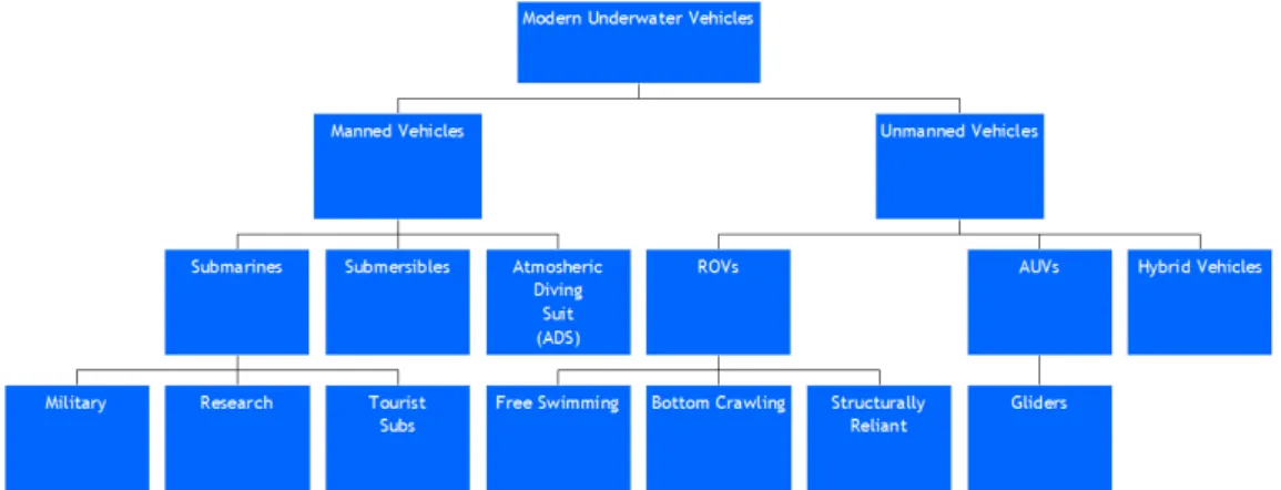
The first knowledge of the oceans came from a direct observation made from vessels, later air-planes, and finally from instruments placed in the water. However, these techniques only work on the surface [1], which falls short of what underwater exploration is all about. According to Steinar Ellefmo [2]: ”There are large unexplored ocean areas, and there is an enormous amount we do not know about them. We actually know more about the moon than the seafloor”. Underwater vehicles (UV) are perfect for the job since they provide a window to the oceans’ deep secrets. Figure 1.1 divides UVs into two categories: manned vehicles and Unmanned Under-water Vehicle (UUV). UUVs are subdivided in Remotely Operated Vehicles (ROVs), Autonomous Underwater Vehicles (AUVs), and hybrid vehicles, which can be autonomous or remotely oper-ated [3].

Figure 1.1: Underwater vehicle class division.

Manned underwater vehicles are human occupied, and despite the ability to perform complex missions, they are still limited to low endurance, due to human physical and psychological lim-itation. Doing an analogy with space exploration, citing Mark Henderson: ”Human beings are poorly designed for the job. They need food, water and oxygen (...) Mechanical probes have none of these shortcomings. They can fly further and faster(...) ” [4].

Remotely operated vehicles are tethered vehicles that draw power from the surface vessel and, as the name suggests, are remotely operated. They are used for routine inspection and maintenance tasks. However, the operation range is limited by the size of the umbilical cable, and as the cable size rises the drag upon itself and the signal delay increases as well, making it difficult to maneuver, requiring a skilled pilot for the task [1].

(22)

In contrast, autonomous underwater vehicles are systems that carry their power supplies and are fully autonomous, releasing the vehicle from the surface vessel and therefore eliminating the costly handling gear, which a tether entails. However, the absence of a human operator narrows AUV operations to its control system, computing, and sensing capabilities. Robustness in control is mandatory to allow the feasibility of such tool [5].

The AUV concept started to be studied in the 60s [6]. The SPURV, Self-Propelled Underwa-ter Research Vehicle, developed at the University of Washington, is the first reported AUV [7]. In the following decades (1970 to 2000) advances outside the AUV community greatly affected the AUV development [6]. The small low-power computers enabled the guidance and control algorithms implementation on autonomous platforms. Proof Of Concepts (POC) prototypes were tested and evolved to the first generation of operational systems able to accomplish predefined objectives. Autonomous Oceanographic Sampling System (AOSN) is an example of that [8]. In this decade, the AUV technology commercialization is becoming a near reality [6]. Currently, there are different solutions for different applications. Marport’s AUV SQX-500, Girona 500 from University Of Girona Center for Research Underwater Robotics (figure 1.2) and SeaBED from Woods Hole Oceanographic Institution (figure 1.3) are examples of multiple body AUVs.

Figure 1.2: SQX-500 AUV (left) and Girona 500 AUV (right) (adapted from [9][9]).

Figure 1.3: Seabed AUV (adapted from [9]).

In May 2009, Portugal submitted a proposal to the United Nations to expand the continental shelf beyond the 200 nautical miles from the coastline [10]. Having tools for exploration and monitoring is therefore essential. In that sense, CEiiA (Centre of Engineering and Product De-velopment), in collaboration with other partners, preceding actual and forthcoming demands,

(23)

started to develop an AUV [11].

1.1 The AUV

CEiiA is a non-profit organization, located in Porto, Portugal. In September 2015, a consortium led by CEiiA started the development of a lightweight AUV (figure 1.4) with the main goal to reinforce the national capacity for mobile autonomous deep-sea exploration and monitoring [11]. Capable of a NDD1_{of 3000 meters, the AUV follows a double-hull configuration.}

Figure 1.4: 3D model of the developed AUV at CEiiA (courtesy of CEiiA).

Payload

The vehicle’s payload is distributed by both hulls. The batteries are on the lower hull and the necessary dry systems and sensors on the upper hull. For the purpose of navigation, the AUV is equipped with the following sensors:

• Depth Cell - This system allows the determination of the vehicle’s depth, based on pressure values;

• Doppler Velocity Log (DVL) - This device uses the Doppler principle [13] to determine the velocity of the vehicle;

• Magnetometer - This device determines the magnetic north;

• Inertial Navigation System (INS) - Through inertial measurement units (IMU), accelerom-eters and gyroscopes, this system calculates the current position, with the knowledge of the initial position;

• Underwater Altimeter - This device sends acoustic signals towards seafloor, and captures the ”reflected” signal. The time between measurements, and knowing the speed of sound in water, the vehicle altitude is calculated.

For the propulsive system, the AUV has four identical thrusters. Two are placed on the vertical plane and the other two on the horizontal plane. The vertical thrusters are located in both of the hulls: the forward thruster is embedded in the lower body and the aft thruster on the

1

(24)

upper. The horizontal thrusters, as can be seen in the figure 1.4, are located in the aft horizontal fairing.

Mission

According to [11], the system was mainly designed to comply with three missions scenarios: 1. Data download and water column profiling, figure 1.5;

2. Resource exploration and mapping, figure 1.6; 3. High resolution habitat mapping, figure 1.7.

With respect to operational scenario, the AUV mission is divided into:

1. Dive - In traditional submarines, the dive maneuver is accomplished through ballast tanks. By the ”in hail” of water, negative buoyancy is achieved, allowing the dive. For this AUV, these compartments do not exist, and the scenario of using the vertical thrusters to reach the depth goal is nonviable, concerning energetic consumption. Therefore, the AUV carries an extra mass in the bow, allowing the descending movement, with nose down attitude. By reaching the predefined operational depth, the extra mass is released, and the residual buoyancy is achieved. Through this stage, it is possible to accomplish mission scenario (1). 2. Data acquisition - During this stage, mission scenarios (2) and (3) can be performed. 3. Ascent - Although the residual buoyancy will always bring the AUV to the surface, and to

avoid energy wasting to speed up the ascent, the AUV carries an extra mass in the stern. When the data acquisition is over, the mass is released and the ascent will begin. Given the fact that the center of buoyancy is aft the center of gravity, the ascent will happen with nose down attitude. Therefore, on the surface, the GPS, global positioning system, which is located in the upper hull’s vertical fin, is above the water line, ensuring the continuous position transmitting.

(25)

Figure 1.6: Resource exploration and mapping (courtesy of CEiiA).

Figure 1.7: High resolution habitat mapping (courtesy of CEiiA).

1.2 AUV Motion Control Techniques Overview

1.2.1 Dynamics

The dynamic model is essential to design the motion control algorithms [14]. The dynamics can be divided into kinematics and kinetics [15]. A brief description will be hereby presented to introduce the general concepts of the AUV dynamic model.

1.2.1.1 Reference Frames and Terminology

To derive the equations of motion that describe the AUV kinematics, the definition of two ref-erence frames is mandatory. The notation that will be used from now on is the one defined [16] by SNAME2, with slight differences, as in [15].

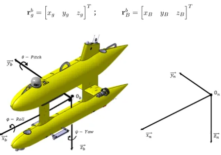
As seen in figure 1.8, the chosen reference frames are:

• The body-fixed {b}, the non-inertial frame, composed by the axes {xb,yb,zb}, and the 0bis chosen, for simplicity, to coincide with the Center of Gravity (CG) of the AUV.

• The local NED (North-East-Down) {n}, the inertial reference frame, composed by the or-thonormal axes {xn,yn,zn}, the origin is represented by 0n.

The CG and the Center of Buoyancy (CB), which is the hydrostatic buoyancy center, are defined with respect to the 0b, and are represented by:

2

(26)

rbg= [ xg yg zg ]T ; rb_B = [ xB yB zB ]T

Figure 1.8: Body-fixed and local NED reference frames.

Therefore, to determine the position and orientation of the vehicle, six independent coordinates are needed, namely (x, y, z, ϕ, θ, ψ), which are expressed in the inertial frame, {n}. For linear and angular velocity, the six coordinates are (u, v, w, p, q, r), and (X, Y, Z, K, M, N ) for control forces/moments, both expressed in the non-inertial frame, {b}. The six motion components can be expressed as in table 1.1, or, in the vector form, as:

• η= [

x y z ϕ θ ψ

]T

expressed in the {n} frame; • ν=[u v w p q r

]T

expressed in the {b} frame; • τ =

[

X Y Z K M N

]T

expressed in the {b} frame.

Table 1.1: SNAME notation for underwater vehicles.

Terminology Forces and Moments Linear and Angular Velocities Position and Euler angles

Motion along xbdirection (Surge) X u x

Motion along ybdirection (Sway) Y v y

Motion along zbdirection (Heave) Z w z

Rotation along xbaxis (Roll) K p ϕ

Rotation along ybaxis (Pitch) M q θ

Rotation along zbaxis (Yaw) N r ψ

1.2.1.2 Kinematic Equations

Kinematics deal with the geometrical aspects of motion and relates the velocities with positions [14]. To transform linear velocities from the body-fixed frame to the inertial coordinate frame, a transformation matrix, J , is defined, resulting in the kinematic equation [15]:

˙ η = J (η)ν (1.1) where: J (η) = [ Rn b(Θnb) 03_×3 03×3 TΘ(Θnb) ] (1.2)

(27)

where Rn

b(Θnb) represents the rotation matrix that allows the linear velocity transformation, from b to n frame, and is defined by [15]:

Rn_b(Θnb) =   

cos(ψ)cos(θ) cos(ψ)sin(θ)sin(ϕ)− sin(ψ)cos(ϕ) cos(ψ)sin(θ)cos(ϕ) + sin(ψ)sin(ϕ) sin(ψ)cos(θ) sin(ψ)sin(θ)sin(ϕ) + cos(ψ)cos(ϕ) sin(ψ)sin(θ)cos(ϕ)− cos(ψ)sin(ϕ)

−sin(θ) cos(θ)sin(ϕ) cos(θ)cos(ϕ)

   (1.3)

The TΘ(Θnb)represents the Euler attitude transformation matrix and is defined as [15]:

TΘ(Θnb) =    1 sin(ϕ)tan(θ) cos(ϕ)tan(θ) 0 cos(ϕ) −sin(ϕ) 0 sin(ϕ)/cos(θ) cos(ϕ)/cos(θ)    (1.4)

Equation 1.4 produces a singularity in pitch, θ =±90◦. Since the vehicle will operate at around θmax≈ ±25◦, Euler representation can still be used. In alternative, the quaternion representa-tion can be used, as shown in [17].

1.2.1.3 Kinetics

Rigid-Body Equations

Kinetics address the relationship between motion and forces. By applying Newton’s law in the body-fixed frame{b}, it is possible to express the rigid-body equation as [15]:

Mrb· ˙ν + Crb(ν)· ν = τrb (1.5)

where Mrbrepresents the rigid-body mass matrix, Crbthe rigid-body Coriolis force, and τrbthe external forces and moments action on the vehicle.

The rigid-body mass matrix is defined as [15]:

Mrb= [ m· I3_×3 −m · S(rgb) m· S(rb g) Ib ] =            m 0 0 0 m· zg −m · yg 0 m 0 −m · zg 0 m· xg 0 0 m m· yg −m · xg 0 0 −m · zg m· yg Ix −Ixy −Ixz m· zg 0 −m · xg −Iyx Iy −Iyz −m · yg m· xg 0 −Izx −Izy Iz            (1.6)

where m is the mass of the vehicle, I3×3 is a 3 x 3 identity matrix; S(rgb)is the skew-symmetric matrix of rb

g, which represents the location of the vehicle’s CG, with respect to the body-fixed frame, (rb

(28)

The Coriolis and centripetal matrix, Crb, is defined as [15]: Crb(ν) = [ 03×3 −m · S(ν1)− m · S(ν2)· S(rbg) m· S(ν1) + m· S(rgb)· S(ν2) −S(Ib· ν2) ] =            0 0 0 0 0 0 0 0 0 −m(ygq + zgr) m(ygp + w) m(zgp− v) m(xgq− w) −m(zgr + xgp) m(zgq + u) m(xgr + v) m(ygr− u) −m(xgp + ygq) m(ygq + zgr) −m(xgq− w) −m(xgr + v) −m(ygp + w) m(zgr + xgp) −m(ygr− u) −m(zgp− v) −m(zgq + u) m(xgp + ygq) 0 −Iyzq− Ixzp + Izr Iyzr + Ixyp− Iyq Iyzq + Ixzp− Izr 0 −Ixzr− Ixyq + Ixp −Iyzr− Ixyp + Iyq Ixzr + Ixyq− Ixp 0            (1.7) where ν1= [u v w]T, and ν2= [p q r]T .

The external forces and moments acting on the vehicle, τrb, can be decomposed in [14]:

τrb= τ + τA+ τD+ τR (1.8)

• τ - Vector of forces and torques created by the surfaces/thrusters. Usually treated as the control input, and defined as:

τ = L· U (1.9)

where, L represents the mapping matrix and U the force vector representing the thrust of each thruster.

• τA- The vector due to the hydrodynamic added mass. In fluid mechanics, an accelerating or decelerating body must move some volume of the surrounding fluid with it. The mass representative of this volume is called the added mass. The added mass vector is defined as [15]:

τA=−MA− CA(ν)ν (1.10) where MAis the added mass matrix, expressed as [15]:

MA=−            Xu˙ Xv˙ Xw˙ Xp˙ Xq˙ Xr˙ Yu˙ Yv˙ Yw˙ Yp˙ Yq˙ Yr˙ Zu˙ Zv˙ Zw˙ Zp˙ Zq˙ Zr˙ Ku˙ Kv˙ Kw˙ Kp˙ Kq˙ Kr˙ Mu˙ Mv˙ Mw˙ Mp˙ Mq˙ Mr˙ Nu˙ Nv˙ Nw˙ Np˙ Nq˙ Nr˙            (1.11)

where, for example, the term Xu˙ represents the hydrodynamic added mass force X along

(29)

forces due to added mass [15]: CA(ν) =            0 0 0 0 −a3 a2 0 0 0 a3 0 −a1 0 0 0 −a2 a1 0 0 −a3 a2 0 −b3 b2 a3 0 −a1 b3 0 −b1 −a2 a1 0 −b2 b1 0            (1.12) Where: a1= Xu˙u + Xv˙v + Xw˙w + Xp˙p + Xq˙q + Xr˙r a2= Yu˙u + Yv˙v + Yw˙w + Yp˙p + Yq˙q + Yr˙r a3= Zu˙u + Zv˙v + Zw˙w + Zp˙p + Zq˙q + Zr˙r b1= Ku˙u + Kv˙v + Kw˙w + Kp˙p + Kq˙q + Kr˙r b2= Mu˙u + Mv˙v + Mw˙w + Mp˙p + Mq˙q + Mr˙r b3= Nu˙u + Nv˙v + Nw˙w + Np˙p + Nq˙q + Nr˙r

• τD- The vector due to lift, drag, skin friction, etc; defined as [15]:

τD=−D(ν)ν (1.13)

with D(ν) being the hydrodynamic damping matrix. If moving with low speed, it is common to use a quadratic approximation [17]:

D(ν) = Dl+ Dq(ν) (1.14) where: Dl=            Xu Xv Xw Xp Xq Xr Yu Yv Yw Yp Yq Yr Zu Zv Zw Zp Zq Zr Ku Kv Kw Kp Kq Kr Mu Mv Mw Mp Mq Mr Nu Nv Nw Np Nq Nr            (1.15) and: Dq(ν) =−            Xu|u|| u | Xv|v|| v | Xw|w|| w | Xp|p| | p | Xq|q|| q | Xr|r|| r | Yu|u|| u | Yv|v| | v | Yw|w|| w | Yp|p|| p | Yq|q|| q | Yr|r|| r | Zu_|u|| u | Zv_|v|| v | Zw_|w|| w | Zp_|p|| p | Zq_|q|| q | Zr_|r|| r | Ku|u|| u | Kv|v| | v | Kw|w|| w | Kp|p|| p | Kq|q|| q | Kr|r|| r | Mu_|u|| u | Mv_|v| | v | Mw_|w|| w | Mp_|p| | p | Mq_|q|| q | Mr_|r|| r | Nu|u|| u | Nv|v|| v | Nw|w|| w | Np|p|| p | Nq|q|| q | Nr|r|| r |            (1.16)

• τR- Represents the hydrostatic restoring force due to gravity and fluid density. According to [15], two forces are considered in the hydrostatics: the buoyancy force, fB, which acts

(30)

upwards, on the CB, and the gravitational force, fg, that acts downwards on the CG.

Archimedes’ principle gives the buoyancy force, B = ρg∇, where ρ is the density of the fluid, g the gravitational acceleration and∇ the volume of fluid displaced by the vehicle [15]. In the {n} frame: f_Bn =    0 0 −B    (1.17)

The gravitational force is derived from the Newton’s 2nd _{law, W = mg, where m is the} mass, and g the gravitational acceleration. In the {n} frame [15]:

f_gn =    0 0 W    (1.18)

For the {b} frame:

f_Bb = Rn_b(Θnb)−1fBn (1.19)

f_gb= Rn_b(Θnb)−1fgn (1.20)

The restoring force vector is equal to [15]:

τR=−g(η) (1.21) And: g(η) =− [ fb B+ fgb rb_Bf_Bb + rgbfgb ] (1.22)

Finally, expanding these equations will result in [15]:

g(η) =            (W− B) sin(θ) −(W − B) cos(θ) sin(ϕ) −(W − B) cos(θ) cos(ϕ)

−(ygW − yBB) cos(θ) cos(ϕ) + (zgW− zBB) cos(θ) sin(ϕ) (zgW− zBB) sin(θ) + (xgW− xBB) cos(θ) cos(ϕ) −(xgW − xBB) cos(θ) sin(ϕ)− (ygW− yBB) sin(θ)

           (1.23)

1.2.1.4 Complete Dynamic Model

By associating the kinematic and kinetic equations and expanding equation 1.8, the complete dynamic model is written as [15]:

(31)

˙

η = J (η)ν (1.25)

Where M = Mrb+ MAand C = Crb+ CA.

The dynamic model can be conveniently arranged to the form ˙x = f (x, t) as: ˙

ν = M−1[−(C(ν)ν + D(ν)ν − g(η) + τ] (1.26)

1.2.2 Motion Control

An autopilot for an AUV is a GNC, Guidance, Navigation and Control, system in its most basic form [15]. The communication sequence can be seen in the figure 1.9 [15].

Figure 1.9: GNC signal flow diagram.

For proper operation, each block should work in accordance with the other. That means imper-fections/errors in one will reduce the efficiency of the other [18]. Since the controller works on guidance data, developing a controller without addressing guidance may not be prudent. Therefore, both of these blocks are covered in this thesis, while navigation block is consid-ered to provide all readings of the current state of the vehicle. A brief literature review was performed to assess the state-of-the-art in this matter.

1.2.2.1 Guidance

According to Fossen [15], guidance is the act of determining the course, attitude and speed of the vehicle, relative to some reference frame, to be followed by the vehicle.

It is the guidance system that decides the best trajectory to be followed by the vehicle, based on target location and vehicle’s capabilities [18]. For a remotely operated vehicle, those refer-ences are sent from a human trained operator. However, for autonomous underwater vehicles, the guidance system plays a vital role in bringing autonomy to the system [18].

Among current solutions, waypoint guidance by Line Of Sight (LOS) is the most common ap-proach for guidance in underwater vehicles [18]. In [19] an improved LOS law, which calculates an additional angle by taking into account AUV’s current position and the next waypoint, is pre-sented. Path following algorithms are also common solutions [15]. A three-dimensional path following algorithm is presented in [20] .

(32)

1.2.2.2 Control

This block is accountable for calculating the necessary forces and moments to achieve the con-trol objective [15].

The AUV’s dynamics is inherently nonlinear and time-variant. The uncertain external distur-bances that the vehicle is subjected to make the AUV controller design task a very challenging one. Therefore, and with the growing need for advanced capabilities and features, a necessity for more capable control systems is mandatory [1].

Numerous control strategies have been developed, being possible to classify them into two main groups, the linear methods and the nonlinear methods [21].

• Linear methods: The linear theory has evolved over the years and powerful design tools, to meet control robustness and stability requirements, were developed. By linearizing the AUV dynamic equations, it is possible to make the control problem more tractable [22]. Despite the nonlinear environment, there are successfully implemented linear controllers in the nonlinear environment. Among the solutions, the most common two will be studied in this thesis.

1. PID (Proportional Integral Derivative) Controller: As stated in [15], a state-of-the-art control system is designed using PID control methods. Jalving [23] proposed a simple PD, to the steering control system, and PI to the speed control system. In [24], to control each Degree Of Freedom (DOF) of the DepthX AUV, 4DOFs, four independent loops were implemented, each loop containing an experimentally tuned PI controller. 2. LQR (Linear Quadratic Regulator): In [25], the dynamics were divided into three subsystems. The dynamic model was linearized around a set of operating conditions, namely, surge velocity u = 1.5m/s, and for the remaining states, to zero. In [26], an LQR controller was proposed to control depth; [27] the Linear Quadratic Gaussian (LQG) was the technique suggested to control the AUV REMUS in the horizontal plane. Finally, [18] proposed an LQG to the autopilot of Hammerhead AUV.

• Nonlinear methods: As stated before, linear techniques can be applied to the nonlinear environment. However, for high-speed motion, nonlinear effects are significant, and lin-ear control may not deliver the required performance [28]. There is a rich collection of alternatives and complementary techniques, to answer the AUV nonlinear needs. Sliding Mode Control (SMC) [21, 29], gain-scheduled LQR approach [30], fuzzy logic [31, 32], NN (Neural Networks) [33], adaptive control [34], nonlinear model predictive control [22], among others; are examples of nonlinear controllers implemented in underwater vehicles [1].

1.3 Motion Control Fundamentals

Some fundamental concepts need to be addressed when developing a motion controller. Namely: operating spaces, actuation properties, and motion control scenarios [35].

1.3.1 Operating Spaces

When designing a controller it is useful to distinguish between two operating spaces: workspace and configuration space [15]. The workspace, also known as the operational space, represents

(33)

the physical space in which the vehicle moves. For a car, the workspace is bi-dimensional (pla-nar position) [35].

The configuration space represents all the possible states of a given vehicle in the workspace [35].

1.3.2 Vehicle Actuation Properties

According to Fossen, Degree-Of-Freedom, DOF, is the set of independent displacements and rotations that completely specify the displaced position and orientation of the vehicle [15]. The type, amount, and distribution of the vehicle’s actuators (thrusters and control surfaces) will determine the actuation of the vehicle. The vehicle can be underactuated or fully actuated [35].

A fully actuated vehicle can control all its DOFs simultaneously independently. In opposite, an underactuated vehicle can only independently control some DOFs simultaneously [15]. However, a vehicle that cannot satisfy a 6 DOF control objective can still achieve meaningful tasks in its workspace [35].

Let us consider an AUV in the horizontal plane. The vehicle needs to follow a path, and it is equipped with one thruster and one rudder, which are the surge and yaw actuators. Although the vehicle does not have active control in sway motion, it can still achieve the control objective with a combination of the action of both actuators. So, even though the AUV is underactuated in the configuration space (three-dimensional: surge, sway and yaw), the vehicle is fully actuated in the workspace (bi-dimensional) [15].

In conclusion, if the vehicle is underactuated in the configuration space but fully actuated in the workspace, it is possible to achieve the control objective [15].

1.3.3 Motion Control Scenarios

To design a motion control system is essential to properly define the control scenarios/objectives, to meet the safe operational requirements of the vehicle. According to [15], motion control ob-jectives are divided into:

• Setpoint regulation: The control objective is to track a desired position, or a desired attitude [15];

• Trajectory tracking: Is a time dependent method, where the system output y(t), is forced to track the desired one yd(t). For an AUV (6 DOF), this means that the signal represents the desired position/attitude, velocity and acceleration as function of time [15];

• Path following: The control objective is to track a predefined path independent of time [15].

Tracking scenario can also be designed as target tracking and path tracking. On target tracking, the control objective is to track the target’s motion that is either stationary or that moves, which in that case, only the instantaneous motion is known. On the path tracking scenario, the control objective is to track a target that moves along a predefined path [35].

These scenarios are typically defined by control objectives given as configuration space tasks. However, for underactuated vehicles, these control objectives should be defined as workspace tasks [15].

(34)

1.3.4 Motion Control Hierarchy

Motion control systems can usually be conceptualized into a three-level hierarchical structure: high-level control, intermediate level control and low-level control, figure 1.10.

The high-level control, labeled as kinematic control is accountable for prescribing vehicle ve-locity commands to achieve the control objective in the workspace [35]. Therefore, this level deals with the geometrical aspects of motion.

Once calculated the reference speeds, the intermediate level deals with the calculation of the forces that the different actuators have to perform to achieve the input references. Kinetic controllers do the calculation of the forces, and the control allocation is responsible for the distribution of the kinetic control commands among the vehicle actuators. These controllers are often designed by model-based methods, and must handle both parametric uncertainties and environmental disturbances [35].

The last level, low-level control, will ensure that the individual actuators will behave as re-quested by the intermediate level control.

Figure 1.10: Motion control hierarchy (adapted from [35]).

For the purpose of this thesis only high and intermediate control levels are addressed.

1.4 Control Systems Fundamentals

1.4.1 Open loop and Closed loop systems

Designing a controller is about making dynamic systems perform certain tasks, to behave in a desired way [36]. Among the control systems configurations, two major will be discussed: open loop and closed loop, or feedback. Although both of the configurations start with the input or reference, and both achieve one output, the open-loop configuration, figure 1.11, cannot compensate for any added disturbance [37]. As an example, if the control system in figure 1.11, represents an electronic amplifier, and the Disturbance 1 represents noise, both input signal and noise will be amplified.

(35)

Figure 1.11: Block diagram of a generic architecture of a open-loop system.

The feedback configuration by taking into account the system’s output, figure 1.12, will correct disturbances, creating a much more accurate and robust control [37].

From this point on, only feedback control systems will be discussed.

Figure 1.12: Block diagram of a generic architecture of a closed-loop system.

The design of control systems usually starts with modeling the system’s plant[36]. To model a system, the designer uses physical laws, like Kirchhoff’s laws for electrical networks, and New-ton’s law for mechanical systems. Such laws will lead to mathematical models that describe the relationship between input and output, I/O.

Therefore, two approaches are available for the analysis and design of feedback control systems, namely: classical, or frequency-domain, technique, and modern, or time-domain, technique [38].

1.4.2 Classical Control

The classical approach is based on converting the system’s differential equation, into a transfer function. Thus generating a mathematical model that algebraically relates the output and the input. The main advantage is that information, like stability and transient response, is promptly provided. Therefore, the variation in the system parameters can instantly be seen and adapted to fulfill the requirements [37].

1.4.2.1 Transfer Function

The transfer function represents the relationship between the system’s input r(t) and system’s output y(t). A physical system that can be represented by an LTI, Linear Time-Invariant, differ-ential equation can be modeled as a transfer function [37].

Considering the feedback system from figure 1.13:

(36)

The transfer function is given by:

G(s) = Y (s)

R(s) (1.27)

where R(s) and Y (s) are the Laplace transforms from r(t) and y(t). Reminding that the Laplace transform is defined as:

L[f(t)] = F (s) = ∫ _∞

0

f (t)e−stdt (1.28)

where s is a complex variable (s = σ + jω). Hence, knowing f (t) and that the integral from equation1.28 exists, it is possible to find the Laplace transform, F (s) from f (t) [37].

This transformation (time-domain to frequency-domain) will result in a polynomial fraction: G(s) = b(s)

a(s) (1.29)

where the roots from b(s) represent the zeros from the system, and the roots of a(s) the poles. Therefore, in the complex plane, the magnitude of G(s) will go to zero at each zero, and to infinity at the poles [39].

1.4.2.2 PID Control Theory

Proportional integral derivative control, figure 1.14, is by far the most common control tech-nique, due to the general applicability to most control systems [40]. In particular, when the plant’s mathematical model is unknown, PID control design methods can still provide satisfactory control. However, in some situations, these may not provide optimal control [38].

Figure 1.14: Feedback block diagram with PID controller.

This controller works on the principle of closed-loop feedback, where the proportional term is linear to the error, the integral term accumulates the error over time, and the derivative measures how fast the error is changing. So, the control law is given by:

u(t) = Kpe(t) + Ki· ∫ t 0 e(τ )dτ + Kd· de(t) dt (1.30)

(37)

The controller also can be parametrized as: u(t) = Kp(e(t) + 1 Ti · ∫ t 0 e(τ )dτ + Td· de(t) dt ) (1.31)

where Ti is called integral time and Td derivative time [40]. The respective transfer function between the input, error, and the output, control law, is then:

U (s)

E(s) = Kp(1 + 1 Tis

+ Tds) (1.32)

The gains are tuned according to system’s requirements. By increasing the proportional gain, the system responsiveness will increase, but for high values, instability can occur, and the steady-state error will remain. Adding the integral term (P I) the steady state can be eradi-cated. However, it can cause overshoot. Therefore, the addition of the derivative term (P ID) increases damping and reduces overshoot [22].

From figure 1.15, it can be seen how the P ID controller works. The integral term accounts for the error up to time t (past), (shaded portion); the proportional term accounts for the instan-taneous value of the error (present); and the derivative estimates the growth, or decay, of the error over time (future) [40].

Figure 1.15: Action of a PID controller (adapted from [40]).

Integrator Wind-up

Linear models can provide an understanding of many aspects of control systems. However, some nonlinear effects should be accounted for when designing a controller, namely the physical limi-tations of the actuators. For example, a thruster has limited speed, and a valve cannot be more than fully opened or fully closed.

When this happens, the feedback loop is no longer doing its job since, at the moment that the system reaches the desired state, the value of the integrator output is still significant. To com-pensate that, the error needs to have opposite sign for an extended period, as shown in figure 1.16. This phenomenon is referred to as integrator wind-up [40].

(38)

Figure 1.16: Wind-up effect.

Literature presents different solutions to this problem [40], two common ones are clamping, or conditional integration which prevents the output from accumulating when the controller output is saturated, and back-calculation (figure1.17). In this last method, when the extra feedback path becomes active (saturation in actuators) the integral term is recomputed, so that its new value helps to stabilize the integrator. It is advantageous to not instantaneously reset the integrator, but instead do it dynamically, with a constant Tt[40].

Figure 1.17: Controller with back-calculation loop (adapted from[40]).

1.4.3 Modern Control

During the 1950s, several authors, including Kalman, began working on the Ordinary Differential Equations (ODEs), as a model for control systems, known as the state-space approach. Allied to these works, the advances in the digital computers allowed the direct work with ODE in the state form. Even though this work’s foundation took place in the 19th_{century, this state-space} approach, for control purposes, is often referred to as modern approach [41].

In the first stage, modern control allows the study of the system’s controllability and observ-ability. Considering an initial time as t0, the terms are defined as:

• Controllability: The system is controllable if and only if exists a control vector that can drive any arbitrary state x(t0)to any other, in a finite interval of time.

(39)

• Observability: The system is observable at a time t if, in the x(t0)state, it is possible to determine this state from the observation of the output, over a finite time interval.

To prove controllability and observability lets consider the linear continuous-time system in the state-state space form, where n is the number of states, p the number of inputs and q the number of outputs [37].    ˙ x = Ax + Bu y = Cx + Du (1.33) where: x = state vector, x ∈ ℜn

u = input or control vector, u ∈ ℜp

y = output vector, y ∈ ℜq

A = system matrix, A ∈ ℜn×n

B = input matrix, B ∈ ℜn×p

C = output matrix, C ∈ ℜq×n

D = feedforward matrix, D ∈ ℜq×p

For the system to be controllable, the controlability matrix Coneeds to have rank n.

Co = [

B AB A2_B _... _An−1_B] _(1.34)

In the same way, the system is observable if, and only if, the observability matrix Q has rank n. O =

[

CT ATCT (AT)2CT ... (AT)n−1CT ]

(1.35)

According with [42], the controlability condition is enough to prove the closed loop stability;

1.4.3.1 Linear Quadratic Regulator

Linear quadratic regulator (LQR) is an optimal feedback controller that in its original form, forces all the states to go to zero. With some modifications can be used to track a reference as seen in the figure 1.18 [39].

Figure 1.18: Linear quadratic regulator system.

To derive the LQR control, controllability and observability need to be ensured [38]. Assuming the state-space form:

˙

x = Ax + Bu (1.36)

Considering that all states are available for the controller, the optimal control problem deter-mines the feedback gain, K matrix, of the optimal control vector:

(40)

The feedback control law for the system is found by minimizing the quadratic cost function, or performance index: J = ∫ ∞ 0 (xTQx + uTRu)dt (1.38)

where Q is a positive-definite (or positive-semidefinite) Hermitian or real symmetric matrix, Q ≥ 0, and R is a positive-definite Hermitian or real symmetric matrix, R > 0. They act like weights, i.e. the Q matrix, for being related with the system state x, will account for the errors’ importance, and R, by being related to the control u, will account for the expenditure of the energy in control signal [38].

The solution to the minimization problem is the positive-definite Hermitian or real symmetric matrix P , which corresponds to the Algebraic Riccati Equation (ARE) [38]:

ATP + P A− P BR−1BTP + Q = 0 (1.39) Resulting in the feedback law:

u =−R−1BTP x (1.40) If working as set point tracker, the feedback law can be given by [39]:

u =−R−1BTP (x− xdesired) (1.41)

With the goal of making the weight selection step more intuitive, Bryson’s method suggests that each element of the diagonal matrices Q and R is the inverse square of the maximum expected value for the variable [42], i.e.:

Q = diag(Qi), Qi= 1 x2 i,max (1.42) R = diag(Ri), Ri= 1 u2 i,max (1.43) Where x2

i,maxand u2i,maxare the maximum expected values for the xi and ui. The design process can be summed up by the following steps [42]:

1. Dynamic system definition (A, B); 2. Weight selection (Q, R);

3. ARE solution (P );

4. Control matrix solution (K); 5. Feedback through equation 1.37.

Integral Action

As in the PID controller, it is also possible to add an integral term to the LQR controller. The basic approach in integral feedback is to create a state within the controller that computes the integral of the error signal, which is then used as feedback term. Lets consider the new variable

(41)

zdefined by [15]:

˙

z = y = Cx (1.44)

Where C matrix is used to extract potential integral states from the state vector x. The system is now defined as:

˙ xa= Aaxa+ Bau (1.45) Where; xa = [ z x ] ; Aa= [ 0 C 0 A ] , Ba= [ 0 B ] (1.46)

The performance is now calculated by: J =

∫ _∞

0

(xT_aQaxa+ uTRu)dt (1.47)

Where Qa = QTa ≥ 0 and R = RT > 0are the weighting matrices. Then the solution to the LQR setpoint regulation is given by:

u =−R−1BT_aP_∞xa (1.48) Where P_∞is the solution to the Riccati equation:

P_∞Aa+ ATaP∞− P∞BaR−1BaTP∞+ Qa= 0 (1.49)

Now, the control objective is to regulate the xa state to zero using u [15]. Reminding that:

z = ∫ _∞

0

e(τ )dτ (1.50)

Remarks about LQR

There are some key characteristics of LQR worth mentioning [18]:

• Excellent stability margins: according to [18], the gain margin up to infinity and over 60 degrees of phase margin. That means robustness for all magnitude of disturbances [43]; • Optimality: Since the closed-loop eigenvalues are found according to the minimization of

the cost function J , there is no need for pole placement and therefore the resulting value is optimal;

• Unique analytical solution.

1.4.4 Stability

The first and most important question about the various properties of a control system is whether it is stable or not. An unstable control system is useless and potentially dangerous [28]. There-fore, every control system whether linear or nonlinear involves a stability problem and must be addressed properly [28].

(42)

1.4.4.1 Linear Systems

Concerning linear time-invariant systems, there are two concepts that need to be addressed: natural response and forced response.

The natural response describes the way that the system dissipates or acquires energy. The nature of this response only depends on the system, not on the input. Contrarily, the forced response is dependent on the input [37]. For an LTI system, it is allowed to say [37]:

Output response = N atural response + F orced response (1.51)

Using these concepts, a system is:

• Stable if the natural response approaches zero as time goes to infinity;

• Unstable if the natural response grows without bounds, as time goes to infinity;

• Marginally stable if the natural response neither decays nor grows but remains constant or oscillates as time goes to infinity.

Therefore, the definition of stability states that only forced response remains as the natural tends to zero [37].

Considering the natural response stability, many techniques, such as solving a differential equa-tion or taking the inverse Laplace, enable the evaluaequa-tion of this output response. However, many are time-consuming and painstaking [37]. A simple and faster method to determine whether the system is stable or not is to analyze the transfer function, namely the poles’ location in the com-plex plane (s = σ + jω), as can be seen in figure 1.19. Therefore, according to [37] a system is:

• Stable if all the poles are located in the Left Half Plane (LHP);

• Unstable if one or more poles are located in the Right Half Plane (RHP); • Marginally stable if at least one pole is located in the imaginary axis (jω).

Figure 1.19: Stability in the complex plane.

Looking now at stability from the perspective of state-space. Considering the linear system: ˙

x = Ax (1.52)

The solution is given by [44]:

x(t) = e(t−t0)A_x

(43)

where x0is the initial state. The exponential of a matrix is defined by the Taylor series [44]: eX= I + X + 1 2X 2₊ 1 3!X 3_{+ ...} _(1.54)

By assuming that the matrix X, with the dimension n× n, has n distinct eigenvectors, i.e is non defective, the solution is given by [44]:

eX= P eΛP−1 (1.55)

where Λ is the eigenvalues diagonal matrix and P the matrix of eigenvectors. Applying now to equation 1.53:

x(t) = P e(t−t0)Λ_P−1 _(1.56)

where the quantity e(t−t0)Λ_{, namely the values of Λ, will determine if the system converges to}

the origin. Therefore, the linear system is:

• Stable if all eigenvalues of A are strictly in the left-half complex plane;

• Unstable if at least one eigenvalue of A is strictly in the righ-half complex plane;

• Marginally stable if all eigenvalues of A are strictly in the left-half complex plane, but at least one is on the imaginary axis jω.

1.4.4.2 Nonlinear Systems

Physical systems are inherently nonlinear. However, no universal technique has been devised for the analysis of nonlinear control systems [28]. However serious efforts have been made to provide the right tools for this task [28]. Among those tools is the Lyapunov theory. The basic Lyapunov theory is comprised of two methods to address the nonlinear system stability, the indirect method, and the direct method [28]. For this thesis purpose, only the indirect method will be addressed.

According to Lyapunov, a system is stable if it starts near an equilibrium point and stays around it ever after [28]. Since nonlinear systems may exhibit much more complex behavior than the linear systems, some additional/refined stability concepts are required.

Asymptotic Stability and Exponential Stability

In some systems, knowing that the state will stay in the neighborhood of the equilibrium is not enough. Therefore it may be a necessity to understand if the state actually converges to the original value. Hence, [28]:

An equilibrium point is said to be asymptotic stable, in addition to the Lyapunov stability, if the states that start close to the equilibrium point actually converge to it.

In many application, there is a need to estimate how fast that convergence occurs. There-fore [28]:

(44)

An equilibrium point is said to be exponentially stable if there is two strictly positive num-bers α and λ such that:

∀t > 0, ∥x(t)∥ ≤ α∥x(0)∥e−λt _(1.57)

where λ is a positive number and it is called as the rate of exponential convergence.

Linearization and Local Stability

The nonlinear system can be linearized around an operating point, or equilibrium point, through a Taylor expansion, and then linear control techniques can be used to control the system. The Lyapunov indirect method, or Lyapunov’s linearization method, is concerned with local stability of the nonlinear system. This method justifies the use of linear control techniques on nonlinear systems. Therefore, the Lyapunov indirect method states that [28]:

• If the linearized system is strictly stable (i.e all eigenvalues of A are strictly in the left-half complex plane), then the equilibrium point is asymptotically stable for the actual nonlinear system.

• If the linearized system is unstable (i.e at least one eigenvalues of A is strictly in the righ-half complex plane), then the equilibrium point is unstable for the actual nonlinear system.

• If the linearized system is marginally stable (i.e all eigenvalues of A are strictly in the left-half complex plane, but at least one of them is on the imaginary axis jω), then one cannot conclude about the linear approximation.

1.4.4.3 Stability Margins

Knowing that the system is stable, in practice, is not enough [40]. Control design is usually done based on mathematical models or through experimental tests in a controlled environment. Both of these methods may not consider all the process variations that can affect the control system. Since the designer cannot have perfect knowledge of the process variations margins must be accounted [43].

First the concepts of phase and gain need to be addressed.

Considering a LTI system G(s). Assuming that the system is subjected to a sinusoidal input [40]:

u(t) = sin(ωt) (1.58)

the output is distorted based on the properties of G(s). For an LTI system, the distortion is presented in two ways: in the magnitude of the signal and in the phase of the signal. The response will be in the form [40]:

y(t) = A(ω)sin(ωt + ϕ(ω)) (1.59)

where A(ω) is the amplitude, and ϕ(ω) the phase shift [40]. The gain is the proportion of the magnitude of the output, to the magnitude of the input at steady state, and phase is the shift of the signal, measured as an angle [43].

(45)

Considering a closed loop system G(s), the transfer function is given by [43]: G(s)

1 + G(s) (1.60)

Reminding that the instability happens if at least one pole is on the Right Half Plane (RHP), it is concluded that this system is unstable if 1 + G(s) = 0, which corresponds to the case where G(s) =−1. Therefore, G(s) must be kept away from −1 for the closed loop system to be stable. This condition corresponds to the case where the gain of the system is 1, or 0dB, and the phase is−180◦because it flips the input upside down [43]. Margin corresponds to how far away from this point the system is.

Gain and phase margins are the amount of gain and phase that can be added to the system be-fore it goes unstable. These margins can be inferred from a Bode plot [43]. However, since the system is subjected to external disturbances, some results may mislead the designer to assume that the system is robust. Therefore, sensitivity is as important to analyze, like gain and phase margin.

Considering the simplified system in figure 1.20.

Figure 1.20: Closed loop system subjected to external disturbances.

The transfer function of the system is [43]: Y (s) = C(s)G(s)

1 + C(s)G(s)R(s) +

1

1 + C(s)G(s)N (s) (1.61)

where N (s) represents the disturbances. The sensitivity function is given by the second term of this equation. Using this result, it is possible to determine the process sensitivity across the spectrum of frequencies. According to [43], the typical values of maximum sensitivity are in the range of 1 to 2. Closest to 1 represent a more conservative controller and closest to 2 a more aggressive controller.

(46)

1.5 Purpose and Contribution

Control systems are an integral part of the modern society [37]. Being able to develop a control system is being capable of understanding the system at its most basic level.

For autonomous vehicles, there is a continuous demand for advanced features. Therefore, the control system design must be able to provide the right performance, ensuring both task accom-plishment and the integrity of the system.

Developing a control system for an underwater vehicle is not straightforward. The highly non-linear underwater environment [45] makes the mathematical modeling of the vehicle a complex task and the outcome may not be an accurate representation of the AUV’s dynamics, affecting the controller performance. It is therefore paramount to devote the necessary effort to develop a control that can be robust to disturbances.

In this context, the purpose of this thesis is to, among the fields of study that the AUV de-velopment entails (figure 1.21), design and analyze two control solutions for the AUV being developed at CEiiA. This work is aimed at increasing CEiiA’s capabilities in the field of control for underwater vehicles.

Figure 1.21: AUV’s fields of study.

An overview of the controllers shows that state-of-art motion control systems are usually de-signed using PID control methods [15]. However, more advanced control systems have been devised. Example of that is the LQR controller. Therefore, two control designs are proposed based on both of these methods. Since the controller can only be as good as its guidance inputs, it will be proposed two guidance solutions, one based on waypoint following and other on path following. For the simulation/validation purpose, the nonlinear model devised in [17] will be used.

Robust Controller Design for an Autonomous Underwater Vehicle

UNIVERSIDADE DA BEIRA INTERIOR

Engenharia