magnetic and electric sensors. Most of the prior works have focused on extracting point or line features from mechanically scanned imaging sonar (MSIS). Meanwhile, few papers introduced small suspended obstacles in experiments to simulate the real operation environment for AUVs.
This paper describes a novel underwater mapping and localization algorithm by MSIS in confined underwater environment with obstacles. In this study, Super SeaKing DST Sonar was chosen according to the principle of building a low cost and low weight AUV. It can generate a-fan-shape beam and rotate the beam through a series of small angles. The scanned area is represented by a two-dimensional colour image. The selection of small obstacles for the experiments is based on two rules: one is the size of the object is much smaller than the vertical beam width; the other is that ensonification of the object does not result in specular reflection. An algebraic map, representing the surrounding environments is finally generated according to the acoustic image. The proposed algorithm, based on mathematical morphology image processing and least squares curve fitting, is fast and performs well under a variety of sonar operating conditions. This paper is organized as follows. Section II exploits the mapping and localization method in details. Section III describes the experimental setup and discusses the results. Finally, conclusions and suggestions for future improvements are presented in section IV.
II. METHODOLOGY
As a monostatic sonar (the projector and the hydrophone are located in the same position), Super SeaKing perceives the surroundings by rotating the sound beam mechanically. Transducer emits sound waves (ping) and then samples its echo as the pulse in time series. The data returned by the Super SeaKing is quantized into a discrete set of intensity values described as bins. Each bin number represents the sampling interval as well as the sound travelling distance. Sonar raw data are formed by stitching received pings together. An acoustic image is then generated by transferring the raw data into 2D Cartesian coordinate system. According to the acoustic imaging procedure, three processing stages are developed to achieve the main aims in this paper.
Stage 1) Pre-processing and Automation: filter out the reverberation in each single returned ping and add artificial signature in the raw data for localization purpose.
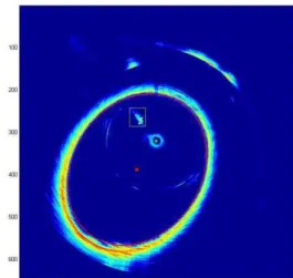
Stage 2) Rapid detection and label: Detect image components in the acoustic image and extract edges of test tank for the mapping. Obstacles are the highlighted by bounding box.
Stage 3)Mapping and localization: Fit the data set using least square technique and then localize the sensor.
A. Pre-processing and Automation
Reverberation represents the energy which is reflected back to the sound source. Likewise, target echoes are just a special case of reverberation [11]. Unwanted reverberation and ambient noise form the background against the targets in
acoustic images. In a structured environment the ambient noise is really small and can be neglected, reverberation is mostly responsible for creating the interfering background. Surface and bottom reverberation are described as boundary reverberation which are dominant components of the reverberation in most shallow water environments [11]. Discrimination boundary reverberation from small obstacles is relatively hard in an acoustic image because their features are similar to each others. Since the reverberation energy may inadvertently cause false alarms and bias the mapping results, a filter is designed to filter out the reverberation energy in each single ping.
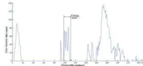
Fig. 1 plots the echo intensity versus the distance of a single ping in a shallow water environment. In Fig. 1, a high amplitude segment can be observed from Bin1 to Bin18. These values near the sensor are phantom detections caused by the sensor itself. Their intensities will be replaced by zero, which represents a no echo return. A complete ping can be partitioned into several segments by its pulse length (from zero to zero). Each segment represents the return energy from the specific ensonified surface of an object.
Fig. 1 One single ping received by the sonar in a shallow water environment.
In structured environments, specular reflection commonly occurs since the boundaries are relatively smooth. When a beam of acoustic signals reaches the edges, most energy will reflect in the specular direction and only a small amount of energy will return to the source. Therefore, if a segment in a ping has low amplitude and spread in a short distance, it may be classified into boundary reverberation. In a similar vein, if a segment has high amplitude and spreads over a wide distance, it may be caused by an object. Fig. 2 compares the difference between the boundary reverberation and a real rigid sphere (18mm in diameter).
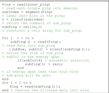
In this case, the maximum intensity of reverberation and target are 41 and 65, respectively. An intensity thresholding method can eliminate the reverberation but it will simultaneously attenuate the echo from objects. Such operations may result in the missing detection of small obstacles. Further, one simple threshold may be not suitable since the intensity of reverberation varies in time and range. On the contrary, the pulse length of a real target is much wider than the boundary reverberation in each ping. In practical sonar performance, energy span of reverberation is commonly less than four bins. An energy span thresholding is therefore designed to automatically filter out the reverberation in each single ping. A pseudo code for the automated filter is shown in Fig. 3.
Fig. 3 Automated reverberation suppression filter
Raw data replay from sensor is in the form of a gray colour image matrix. Echoes of emitted pings are aligned vertically according to the transducer orientation (bearing). Each row represents a specific bearing and each column represents rang measurement results (echo intensity). In this paper, a 360 degree sonar scan is described as one frame. Fig. 4 shows one frame raw data by pseudo colour.
Fig. 4 Sonar raw data. The size of this image frame is 200×248 pixels, which means the scan step was 1.8° and 200 pings were emitted from the transducer. There are 248 bins were obtained in each ping.
The localization method is based on the following two conclusions:
1. The arrangement of the raw data is similar to the polar coordinate system, since each point on the two-dimensional plane represents an angle and a distance. Although sonar raw data cannot illustrate the operational environment directly, it indicates the initial point where acoustic waves were projected. Since the range measurement of the first bin in each row is close to zero meters, it is possible to assume that the first column in the raw data represents the sonar centre.
2. The transformation from a polar coordinate system to a cartesian coordinate system will only change the location of each point but remain colour intensity unaltered. Namely, if a point which intensity is unique in the raw data, a corresponding point with same intensity can be easily extracted in the Cartesian space.
Therefore, if replace the first column of the raw data by artificial signatures, localization problem will eventually become searching problem in the Cartesian coordinate system. Obviously, searching a specific element in a matrix is much simple and easy to achieve. Since all the elements in the raw data are in the range of 0-255, to ensure artificial markers are easily detectable in each frame, the values for markers are assigned to 1000, which are distinctly higher above other elements. When the sonar raw data are represented in a two-dimensional x-y Cartesian plane, sensor position can be easily located by traversing the image and find out the peak values in image matrix. Fig. 5 illustrates the pseudo code for automated localization.
Fig. 5 Automatic sonar sensor localization in an acoustic image
B. Rapid detection and label
Cartesian representation will reproduce the image in a two-dimension plane with x-y space. Images reproduced in a cartesian coordinate system are easy to interpret. A digital acoustic image is a grey level image. The elements of the intensity image have integer values in the range [0, 255]. Targets in the image commonly have higher intensities than the background. To isolate the targets from the background, a simple and effective method is through thresholding. Thresholding will convert an intensity image to a binary image Ping = read(sonar_ping)
% read each single ping into memory; subIndex = segment(Ping)
% label zero bins in the ping; n = sizeof(subindex)
% return the numbers of sub_ping; subPing = cell(n,1)
% construct a cell array for sub_ping;
for i = 1 to n
subPing{i} = read(Ping); % read data into sub_ping
[subRow, subCol] = sizeof(subPing{i}); % return the size of sub_ping
% subCol is the energy span
if(subCol<4) % automatic selection subPing{i} = zero;
end
% if energy span less than four bins % sub-ping will be zero
end
for i = 1 to n
Ping = read(subPing{i});
end % restore the filtered data into ping
Im = imageread(sonar_raw_data); % read the raw data into memory; [row, col] = sizeof(Im);
% return the size of the image matrix; for i = 1 to row
% add markers in each single ping;
Im(i,1) = 1000; % assign marker to 1000; end
acoustic_image = drawImage(Im);
% reproduce the acoustic image in X-Y coordinate filter = mediafilter(3);
% generate a 3×3 media filter
filter_image = imfilter(acoustic_image, filter); % smooth the acoustic image by media filter peak = maximum(filter_image);
by turning all pixels below some threshold to zero and all pixels above that threshold to one. Otsu method [12] is clustering-based global thresholding method for automatic threshold selection from a histogram of the image. It is easy to perform because only the zeroth and the first cumulative moments of the grey level histogram are utilized. The threshold is determined by minimizing the weighted within-class variance of the black and white pixels. Fig. 6a shows the acoustic image after pre-processing and Fig. 6b shows the binary image after the Otsu thresholding.
Fig. 6 (a) One frame acoustic image in x-y plane after pre-processing. (b) Binary image after Otsu thresholding
In a binary image, there are only two Boolean values for
each pixel: ‘0’ or ‘1’. In this study, the foreground set (pixels),
which comprise all objects in an image is referred to as white
colour (‘1’). The foreground objects can be easily labelled and categorised by their size. The rest complement sets are called the background, which are black in colour (‘0’). To map the environment, it is necessary to obtain the inner edges of the test tank. The foreground objects are firstly dilated by a 3-STREL-octagonal structuring element to fill small holes and smooth the contour. Under the assumption that the largest object in the binary image is the test tank, all the other foreground objects can be eliminated from the binary image (refer to Fig. 8a). A sequence of logical operations is secondly executed to acquire the boundaries of the tank. Canny edge detection algorithm [13] is finally performed to detect the edge points of the pool in the binary image.
Fig. 8 Test tank edge detection procedure. (a) Test tank detected by the sensor. (b) Filling result by region grow. (c) Inner boundaries of the test tank
after logical operations. (d) Edge detected by Canny for mapping only.
Since the tank has been successfully detected from the acoustic image, the multiple reflections outside the tank can be identified and assigned to the background. Mathematical morphological approach is an effective way for analysing the geometric structures which are inherent from the image. The method used to detect small targets inside the tank is inherited from previous study [14]. A 4-STREL-disk structuring element is firstly dilated with the foreground regions in the binary
image. Small regions, whose centroids are close to each other, can expand and fuse together after the dilation. Again, regions are then categorised by the area size (the actual number of pixels in the region). If the size of a region is smaller than a predetermined value (in this case, 100 pixels), the region will be classified as noise and then will be rejected from the foreground region. The rest of the regions are finally marked as targets. Considering the AUV navigation and obstacle avoidance, a bounding box, the smallest rectangle which contains an obstacle is generated to set a secure area around the targets.
C. Mapping the environment and sonar localization In fact, the rough map has been obtained after stage 2. At this stage, an algebraic model of the environment is generated for high accuracy localization and AUV navigation purpose. The method for the algebraic map is based on linear least squares ellipse fitting. Ellipses in two-dimensions can be represented algebraically by (1)
2 2
( , ) a x= =0
(1)
F x y ax bxycy dxey f
A least squares solution is to minimize the sum of squared algebraic distance D over a set of N data points by an appropriate constraint:
2
1
( , x ) =min
(2) N
i i
D F a
There are a number of different approaches to find solutions for such constraint. For comparison purpose, the coefficients output of Bookstein’s [15] and Ganders’ approach [16] are listed in the Table. 1.
Method Center.x Center.y Major axis (pixels)
Minor axis (pixels)
Bookstein 243.686 199.540 153.3503 122.0485
Gander 243.686 199.540 153.3451 122.0521
Table. 1 coefficients output of ellipse fitting
Table.1 clearly indicates that there is only a tiny difference between these two ellipse fitting approaches. To produce the results listed in Table 1, Ganders’ approach is approximately two times faster than Bookstein’s. It is therefore chosen to fit the data set. Since the geometric centre of the elliptic tank is obtained, the sonar position can be localized. Fig. 9 illustrates the final results.
III.EXPERIMENTS AND RESULTS
A. Experimental setup
Experiments were conducted in an elliptical cylinder test tank (see Fig. 10). Three hard plastic buoy balls were used as obstacles because their target strengths were relatively independent of the orientation. Their circumferences are 88mm (×2) and 56mm, respectively. Weights on the bottom of the pool were attached to the spheres by ropes. The depth of the three objects was set to be 3.0m below the water surface. The sonar was hung by the claw and suspended at 2.5m depth in three different positions and the scan range was set to 6 meters. At each position, over 20 image frames were taken. During sampling, sensor control factors, the number of objects and their positions were varied.
Fig. 10 Experiment setup B. Results
In the first position, Super SeaKing was operated at 300 kHz and step size was 1.8 degrees. One 56mm sphere was used as a static obstacle in the test tank. The dimensions of the test tank measured by the SeaNet Pro (survey-data-acquisition and logging-software package for the sonar sensor) are 730.7cm × 579.5cm (Major axis × Minor axis). Fig. 11 shows the mapping results. Table 2 shows the coefficients of the elliptic map in eight continuous frames. where:
No. – number of frames SC – centre of the sonar sensor TC – centre of the test tank
MaL – Major axis length of the test tank in centimetres MiL – Minor axis length of the test tank in centimetres PO – Orientation of the elliptic pool in radian
Fig. 11 Mapping results when sonar was located at the first position. Red ellipse indicates the algebraic map. Sensor position is highlighted by square in green and obstacle is depicted inside yellow bounding box.
No. SC TC MaL MiL PO
1 (321,324) (278.09,386.42) 710.43 578.73 -0.92 2 (321,324) (278.03,387.89) 714.26 578.62 -0.98 3 (321,324) (277.68,387.89) 715.59 580.47 -0.96 4 (321,324) (278.14,387.68) 711.08 578.88 -0.95 5 (321,324) (277.69,388.21) 712.08 579.73 -0.97 6 (321,324) (278.00,387.67) 710.12 579.95 -0.95 7 (321,324) (277.84,387.69) 710.86 579.32 -0.96 8 (321,324) (277.81,388.06) 711.23 579.32 -0.97
Table. 2 Coefficients of the ellipse tank and sonar position
In the second position, Super SeaKing was operated at 670 kHz and step size was 3.6 degrees. Two spheres were used as dynamic obstacles in the test tank. The dimension of the test tank measured by the SeaNet Pro is 735.7cm × 581.5cm (Major axis × Minor axis). Fig. 12 shows the results and Table 3 shows the coefficients of the elliptic map in eight continuous frames.
Fig. 12 Mapping results when sonar was located at second position.
No. SC TC MaL MiL PO
1 (257,252) (243.59,199.62) 723.04 575.49 -1.76 2 (257,252) (243.59,199.62) 723.52 574.87 -1.76 3 (257,252) (243.70,199.66) 723.74 575.22 -1.76 4 (257,252) (243.63,199.57) 724.03 574.99 -1.76 5 (257,252) (243.46,199.71) 723.64 574.92 -1.77 6 (257,252) (243.49,199.50) 723.52 575.31 -1.76 7 (257,252) (243.45,199.61) 724.07 574.74 -1.77 8 (257,252) (243.43,199.56) 722.98 575.18 -1.77
Table 3 Coefficients of the ellipse tank and sonar position
In the third position, Super SeaKing was operated at 670 kHz and step size was 1.8 degrees. Sonar scan sector is 180 degree only. Three spheres were used as static obstacles in the test tank. The dimension of the test tank measured by the SeaNet Pro is 734.7cm × 572.74cm (Major axis × Minor axis). Fig. 13 shows the results and Table 4 shows the coefficients of the elliptic map in eight continuous frames.
No. SC TC MaL MiL PO
1 (498,491) (469.06,397.15) 733.87 572.27 -1.87 2 (498,491) (468.61,398.07) 735.82 573.33 -1.87 3 (498,491) (469.19,396.67) 733.01 572.02 -1.87 4 (498,491) (468.49,398.27) 736.58 573.39 -1.87 5 (498,491) (469.46,397.73) 735.70 573.08 -1.87 6 (498,491) (469.04,397.61) 734.94 572.56 -1.87 7 (498,491) (468.99,397.45) 734.14 572.73 -1.87 8 (498,491) (469.21,397.06) 733.82 572.54 -1.87
Fig. 13 Mapping results when sonar was located at third position.
C. Discussion
In this paper, the dimensions of the elliptic test tank are obtained by three different means:
a) Design dimensions (original dimensions), which are 760cm×600 cm (Major axis × Minor axis);
b) SeaNet Pro measurements, which are 728.2cm×580.5 cm (Major axis × Minor axis) on average;
c) Ellipse fitting results, which are 717.4cm×577.4 cm (Major axis × Minor axis) on average.
Since the original dimension is the standard to be compared against, a majority of measurement errors are from the current sonar beam model and the geometrical shape (elliptic paraboloid) of the test tank. A-fan-shape beam has a 3.6 degree horizontal beamwidth and 40 degree vertical beamwidth. As the beam hits the boundaries of the test tank, specular reflections occur at the vertical tangent surface. To plot the horizontal sonar images, the tangent surface is compressed into one point. Such acoustic imaging strategy causes the blurred boundaries in the image and therefore results in the measurement errors. Moreover, in this study, the real boundary of the test tank in each single beam is assumed to be at the place where first specular reflections have occurred. Hence, the silhouette image of the test tank will affect the final ellipse fitting results. In Fig. 7, the inner boundaries acquired by the sonar have several bumps. Therefore, the measurement results are smaller than the others.
IV. CONCLUSIONS AND FUTURE WORK
This paper presents an efficient algorithm for underwater mapping and localization using acoustic sensor in an enclosed and elliptical environment. Boundary reverberation and multiple reflection, which interfering the detection of small obstacles, are successfully eliminated from the acoustic image. Suspended underwater obstacles and the boundary of the enclosed environment are mapped mathematically. The localization is then achieved by the algebraic map without other sensor data. Experiments show a very satisfying result for AUV’s navigation and obstacle avoidance purposes.
When the sonar sensor is mounted on a real vehicle, the acoustic image obtained will be distorted because the sensor-scanning rate is relatively slow in comparison with the vehicle motion. Such distorted acoustic images will lead to poor results. However, if the position of each beam is known, the
distortion caused by the motion can be compensated. With other sensor data, such as Doppler Velocity Log (DVL) and compass, the displacements and rotations can be incorporated to correct the distorted acoustic image. This is one of the prospects for future research and development.
ACKNOWLEDGMENT
The project work has been carried out jointly by the robotics group at the School of Mechanical Engineering, the University of Adelaide and Maritime Operation Division (MOD), Defence Science and Technology Organisation (DSTO). The authors would like to acknowledge the financial and in-kind support received from DSTO, (MOD). Also, thanks to the workshop staff at the School of Mechanical Engineering for their technical support.
REFERENCES
[1] J. Leonard, A. Bennett, C. Smith, and H. Feder, "Autonomous Underwater Vehicle Navigation," 1998.
[2] M. M. Hunt, W. M. Marquet, D. A. Moller, K. R. Peal, and W. K. Smith, "An Acoustic Navigation System," 1974.
[3] P. E. An, A. J. Healey, S. M. Smith, and S. E. Dunn, "New experimental results on GPS/INS navigation for Ocean Voyager IIAUV," 1996, pp. 249-255.
[4] L. Lucido, J. Opderbecke, V. Rigaud, R. Deriche, and Z. Zhang, "A terrain referenced underwater positioning using sonar bathymetricprofiles and multiscale analysis," 1996. [5] M. Sistiaga, J. Opderbecke, and M. J. Aldon, "Depth image
matching for underwater vehicle navigation," 1999, p. 624?29. [6] J. Nie, J. Yuh, E. Kardash, and T. I. Fossen, "On-board
sensor-based adaptive control of small UUVs in very shallow water,"
INTERNATIONAL JOURNAL OF ADAPTIVE CONTROL AND SIGNAL PROCESSING, vol. 14, pp. 441-452, 2000.
[7] M. Caccia, G. Bruzzone, and G. Veruggio, "Sonar-based guidance of unmanned underwater vehicles," Advanced Robotics, vol. 15, pp. 551-573, 2001.
[8] H. Durrant-Whyte and T. Bailey, "Simultaneous Localisation and Mapping (SLAM): Part I The Essential Algorithms," Robotics and Automation Magazine, vol. 13, pp. 99-107, 2006.
[9] S. Williams, G. Dissanayake, and H. Durrant-Whyte, "Towards terrain-aided navigation for underwater robotics," Advanced Robotics, vol. 15, pp. 533-549, 2001.
[10] D. Ribas, P. Ridao, J. Neira, and J. D. Tardos, "Line Extraction from Mechanically Scanned Imaging Sonar," LECTURE NOTES IN COMPUTER SCIENCE, vol. 4477, p. 322, 2007.
[11] A. D. Waite, Sonar for Practising Engineers: Wiley Chichester, 2002.
[12] N. Otsu, "A threshold selection method from gray-scale histogram," IEEE Trans. Systems, Man, and Cybernetics, vol. 8, pp. 62-66, 1978.
[13] J. Canny, "A computational approach to edge detection," IEEE Transactions on Pattern Analysis and Machine Intelligence, vol. 8, pp. 679-698, 1986.
[14] Shi. Zhao, Amir. Anvar, and Tien-Fu. Lu, "Automatic Object Detection and Diagnosis for AUV Operation Using Underwater Imaging Sonar", presented at Industrial Electronics and Applications, 2008. ICIEA 2008. 3rd IEEE Conference on, pp. 1906-1911, 2008.
[15] F. L. Bookstein, "Fitting Conic Sections to Scattered Data," Computer Graphics and Image Processing, pp. 56-71, 1979. [16] W. Gander, G. H. Golub, and R. Strebel, "Least-squares fitting of