CREDIT RISK MEASUREMENT OF THE LISTED
COMPANIES IN CHINA BASED ON KMV MODEL
DONG QI
A dissertation submitted as partial requirement for the conferral of
Master in Finance
Supervisor:
Professor: Doutor José Carlos Dias, Professor Auxiliar, ISCTE Business
School, Department of Finance
CREDIT RISK MEASUREMENT OF THE LISTED
COMPANIES IN CHINA BASED ON KMV MODEL
DONG QI
A dissertation submitted as partial requirement for the conferral of
Master in Finance
Supervisor:
Professor: Doutor José Carlos Dias, Professor Auxiliar, ISCTE Business
School, Department of Finance
i
Acknowledgments
At the first, I would like to extend my sincere gratitude to my supervisor, Professor José Carlos Dias José Carlos Dias, for his instructive advice and useful comments on my thesis. I do appreciate his patience and professional instructions.. I am deeply grateful for his help in the completion of this thesis.
Secondly, the database of RESSET from the professional group of Finance in providing sufficient data for my research. Without them the research was not possible.
Finally, my gratitude also extends to my family who have been assisting, supporting and caring for me all of my life. Special thanks to my friends who helped and encouraged me during the difficult course of the thesis.
ii
Abstract
Due to the recent global financial crisis, which triggers a great number of corporate defaults (Moody's, 2009), as well as the innovation in the corporate debt and derivative products, both academics and practitioners have shown renewed interest in default risk modeling. One of the most frequently studied forecasting models is the KMV model, which is derived from the groundbreaking work of Merton (1974) and its most successful commercial variant - KMV model. KMV model is a kind of measuring method which has applied option pricing theory into the risk management of portfolios and then evaluations the corporations‟ credit risk. It has widespread applications in the international financial market.
Since the split-share reform has been carried out for ten years in China, in the current market environment the dissertation chooses some listed companies samples to do an empirical test to see whether KMV model can measure credit risk effectively in the Chinese Financial market. These listed companies are divided into two groups, one is a default group (ST&*ST companies), ST&*ST companies usually have some financial trouble. Another one is a control group (Blue-chip companies), Blue-chip companies are those who have the best performance. Through empirical research, we find out that the KMV model can distinguish the credit risk of ST&*ST listed companies and Blue-chip companies, which illuminates that KMV model is available in Chinese stock market in today‟s entire circumstance.
JEL Classification: C53, G32
Keywords: China, Credit risk, KMV model, Distance to default, Probability of Default,
iii
Resumo
Devido à recente crise financeira global que provoca um grande número de defaults de empresas (Moody`s, 2009), bem como a inovação na dívida corporativa e de produtos derivados, vários académicos e profissionais têm demonstrado um interesse renovado na modelagem do risco de incumprimento. Um dos modelos de previsão mais estudados é o modelo KMV que é derivado do trabalho pioneiro de Merton (1974) e é actualmente muito utilizado na indústria financeira. O modelo KMV é um método que utiliza a teoria das opções para avaliar o risco de crédito das empresas.
Tendo em conta a reforma de split-share que se vem realizando há dez anos na China, form escolhidas para esta dissertação algumas amostras de empresas cotadas para realizar um teste empírico no sentido de verificar se o modelo KMV pode ser utilizado para medir o risco de crédito de forma eficaz no mercado financeiro chinês. Estas empresas são divididas em dois grupos: um é do grupo padrão (empreas ST & * ST), que geralmente apresentam algum problema financeiro. Outra é um grupo de controlo (empresas blue-chip), isto é empresas que apresentam um melhor desempenho. Através da investigação empírica, constatou-se que o modelo KMV pode distinguir o risco de crédito das empresas ST & * ST e empresas blue-chip cotadas.
Classificação JEL: C53, G32
Palavras-chave: China, risco de crédito, modelo KMV, Distance-to-padrão,
probabilidade de inadimplência, do ponto padrão, ST & * ST empresas, empresas blue-chip
iv
Contents
Acknowledgments... i Abstract ... ii Resumo ... iii Contents ... iv List of abbreviations ... viList of Figures ... vii
List of Tables ... viii
Chapter 1 ... 1
Introduction ... 1
1.1 Background and significance of the study ... 1
1.2 Objective ... 2 1.3 Limitation ... 3 1.4 General framework ... 3 Chapter 2 ... 4 Theory ... 4 2.1 Credit risk ... 4
2.1.1 The definition and components of credit risk ... 4
2.1.2 The characteristics of credit risk ... 6
2.1.3 The causes of credit risk ... 8
2.2 Credit Spreads ... 9
2.3 Credit Risk Modeling in Practice ... 10
2.4 Brownian Motion ... 12
2.4.1 The stochastic process ... 12
2.4.2 Standard Brownian Motion ... 13
2.4.3 Geometric Brownian Motion ... 14
2.5 Theoretical Extensions of the Merton (1974) Model ... 15
2.6 KMV model in China ... 17
2.6 Classical credit risk measurement model ... 18
v
2.6.2 Credit rating Models ... 19
2.6.3 Credit Scoring Models ... 21
Chapter 3 ... 23
Empirical Research: Methodology and Data ... 23
3.1 The Moody‟s KMV Approach ... 23
3.1.1 The Expected Default Frequency Credit Measure ... 23
3.1.2 Estimation of the asset value and the volatility of asset return ... 25
3.1.3 Calculate the Distance-to-default ... 30
3.1.4 Compute the probability of default ... 31
3.1.5 Advantage of the Moody‟s KMV model ... 31
3.2 Selection of parameter ... 32
3.3 Data selection ... 33
3.3.1 Data Source... 33
3.3.2 Selection of Default Group ... 33
3.3.3 Selection of Control Group ... 34
Chapter 4 ... 37
Empirical Research: Results and Analysis ... 37
4.1 The calculation and results ... 37
4.2 Statistical tests on default points ... 40
4.3 OLS Regression Model Results ... 40
Chapter 5 ... 43
Conclusion ... 43
Bibliography ... 45
vi
List of abbreviations
BSM
Black-Scholes-Merton
CBRC
China Banking Regulatory Commission
CRA
Credit Risk Ratings
DD
Distance to Default
DPT
Default Point
EDF
Expected Default Frequencies
EAD
Exposure at Default
IRB
Internal Ratings-Based
LTD
Long-term Debt
MDA
Multiple Discriminant Analysis
PD
Probability of Default
RR
Recovery Rate
vii
List of Figures
Figure 1 Factors determining the credit risk of a portfolio ... 6 Figure 2 Typical credit and market return distributions ... 7 Figure 3 Two sample paths of Geometric Brownian motion with different parameters. . 15 Figure 4 Frequency distribution of a firm‟s asset value at the horizon of time H and probability of default... 25 Figure 5 The relationship between equity value and asset value ... 26 Figure 6 The default distance comparison of 2 groups ... 40
viii
List of Tables
Table 1 Moody‟s and Standard and Poor's credit rating ... 20
Table 2 Five types loans and the corresponding case in China ... 21
Table 3 The information of default group and control group ... 36
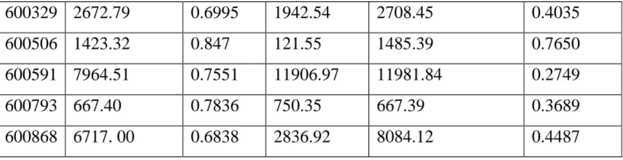
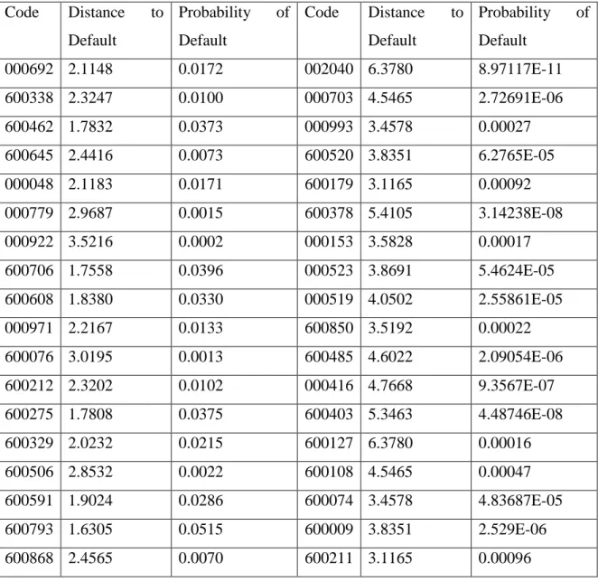
Table 4 The default group (ST&*ST listed companies) basic input data ... 38
Table 5 The control group (Blue –Chip listed companies) basic input data ... 39
Table 6 The estimated of distance to default and probability of default ... 39
Table 7 Comparison of DD and EDF between defaulted group and control group. ... 41
Table 8 Statistic tests among DD and EDF series from two groups. ... 41
1
Chapter 1
Introduction
1.1 Background and significance of the study
Credit risk has been the most important risk faced by the banking industry. According to the World Bank research on the global crisis studies, the most common cause of bank failures is credit risk. From the 1980s, saving and depositing institutions in developing countries going bankrupt like Barings, Daiwa Bank and other financial institutions crisis and the event of huge losses of the United States long-term capital management company. Especially the August 2007 outbreak of the US subprime mortgage crisis led to a number of investment banks and insurance institutions to fail or mess up, and then evolved into a global financial crisis. All of these events have fully demonstrated effective credit risk prevention and management, not only related to a country‟s macroeconomic security, sustainability and health, but also affects the stability and harmonious development of the global economy. Under the impetus of globalization of financial markets and financial innovation, liquidity of bank assets is growing, increasingly diversified of product range, the size of derivative transactions has been expanded, managed and measured research about credit risk in the financial sector has become one of the most challenging, so the research on this subject has a key theoretical value.
"The new Basel Capital Accord" is a comprehensive set of reform measures, developed by the Basel Committee on Banking Supervision, to strengthen the regulation, supervision and risk management of the banking sector. It releases a ratio that must be no lower than 8% of total capital, and the requirement of capital to reflect on the various types of measurement methods of measuring bank risk assets. The Committee proposes to permit banks a choice between two broad methodologies for calculating their capital requirements for credit risk. One alternative will be to measure credit risk in a standardized manner, supported by external credit assessments. Another one is the internal ratings-based (IRB) approach, subjected to certain minimum conditions and disclosure requirements, banks that qualify for the IRB approach may rely on their own
2
internal estimates of risk components in determining the capital requirement for a given exposure. The risk components include measures of the probability of default (PD), loss given default (LGD), the exposure at default (EAD), and effective maturity. China Banking Regulatory Commission (CBRC) required large domestic banks to implement the New Basel Capital Accord, for the credit risk which requires implementing the primary IRB and demands asset coverage over 50%. These have provided banks with a motive for credit risk measurement.
In China, listed companies are the foundation of the stock market, which is an important part of the national economy. The status of listed company‟s credit risk directly related to the healthy development of capital market, which relates to the improvement of our financial system and stable of macroeconomic development. Meanwhile, listed company's credit risk has led more and more investors, regulators and financial institutions to attend.
Researching the credit risk measurement of Chinese listed companies is pivotal because: firstly, from the perspective of commercial banks and other financial institutions, through assessing the credit risk of listed companies which improve the conditions of credit and the accuracy of decisions, managed credit risk effectively. Secondly, from the investor point of view, through assessing the credit risk of listed companies which complete control the conditions of operation and optimize their portfolios, in order to obtain greater profit. Thirdly, from the perspective of the regulatory authorities, through assessing the credit risk of listed companies, listed companies can prevent credit risks more effectively, to strengthen the supervision of the securities market. From the perspective of a listed company through assessing the credit risk of listed companies which can be timelier and more accurate understanding the company's credit risk profile, so as to formulate appropriate management decisions, to improve the company's operational efficiency.
1.2 Objective
In this study, the KMV model is applied to 36 Chinese listed non-financial companies from 2012. The purpose of this paper is to further apply the KMV model with adjusted parameters and initially introduce the market based default calculation of the Chinese
3
stock market. Through comparing the distance to default (DD) and probabilities default (PD) from two types listed companies by the KMV model, this paper aims to find a more effective approach to estimate the default risk in the Chinese stock market and investigate whether KMV model can effectively distinguish credit risk for Chinese companies.
1.3 Limitation
Due to lack of historical statistical data in China‟s credit system, this study focus is on the default distance instead of the actual default rate. Besides, because of data availability, a selected sample of 36 listed companies is included in this study.
1.4 General framework
The structure of the paper is divided as follows. The introduction chapter explains the background of the subject at hand. Chapter 2 presents the theoretical and financial background of the Moody‟s KMV model and previous empirical findings. Chapter 3 explains the methodology, describes the data and examines the parameters setting. The empirical results and discussion appear in chapter 4. Finally, chapter 5 concludes the paper and gives direction for further research.
4
Chapter 2
Theory
According to Altman and Saunders (1999), models assessing credit risk have changed significantly, as investment banks, investors and credit rating agencies apply models that are increasingly more sophisticated. Typically, literature separates between three main branches of credit risk models. Structural models are employed extensively to assess credit risk by utilizing an explicit relationship between the capital structure and default risk (Wang, 2009). Further, accounting models assess credit risk exploiting historical data from financial statements. Lastly, hybrid models are comprehensive models comprising information from structural models, accounting data, macroeconomic variables and rating data (Chan-Lau, 2006). As mentioned, the focus in this thesis is structural models.
2.1 Credit risk
First of all, we introduce the basic information of credit risk, including the definition and components of credit risk, the characteristics of credit risk, and the last one is the causes of the credit risk. These basic credit risk information can help us better understand how to effectively manage credit risk.
2.1.1 The definition and components of credit risk
The credit risk is the risk with which most commercial banks confront; it is also the oldest and the most difficult to manage and control. Credit risk is an investor's risk of loss arising from a borrower who does not make payments as promised. Such events are called default. Another term for credit risk is default risk. Investor losses include lost principal and interest, decreased cash flow, and increased collection costs. Traditionally, from the source point of view, the credit risk can be divided into Counterparty Risk and Issuer Risk.
5
2.1.1.1 Counterparty Risk
Counterparty Risk is corresponding to loan and financial derivatives transactions, because the positions are illiquid and it is difficult (if at all possible) to trade out of them, the analysis period generally uses the whole period of the contract of one year or longer time horizon, etc.
2.1.1.2 Issuer Risk
Issuer Risk refers mostly to bonds, since positions can quickly have traded in the market, the Issuer risk of bonds is computed over a time horizon of a few days – similarly to traditional market risk. The above two types of credit risk is not absolutely isolated, such as credit derivative contracts on with both the above two types of risk.
From the composition point of view, the credit risk is mainly composed of Default Risk and Credit Spread Risk.
2.1.1.3 Default Risk
Default Risk mainly refers to the possibility of a counterparty being unwilling or unable to pay the agreed payment resulted in losses to the other, but even in the default case, there will usually be a part of the debt settlement, the proportion of the liquid
ation is called Recovery Rate (RR).
2.1.1.4 Credit Spread Risk
Credit spread risk means if a counterparty does not default; there is still risk due to the possible widening of the credit spread or worsening in credit quality, by the Jumps in the Credit Spread and Credit Spread Volatility composition specifically.
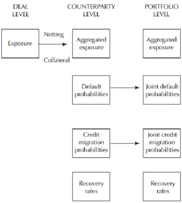
In addition, three groups of factors are important in determining the credit risk of a portfolio. First, Deal – Level factors (Exposure, Default probabilities and Credit migration probabilities) corresponding to a single transaction. Second, Counterparty - Level factors (Aggregated exposure) corresponding to a portfolio of transactions with a
6
single counterparty. Third, Portfolio - Level factors(Joint default probabilities and Joint credit migration probabilities) corresponding to a portfolio of transactions with more than one counterparty. As illustrated in Figure 1
Figure 1 Factors determining the credit risk of a portfolio
Source: Credit: The Complete Guide to Pricing, Hedging and Risk Management
2.1.2 The characteristics of credit risk
Comparing with the market risk, credit risk encompasses three distinct characteristics: return distribution asymmetric, Credit transaction information asymmetry and non-systematic credit risk.
7
2.1.2.1 Return distribution asymmetric.
Under normal circumstances, fluctuations in market prices are the center of its expectations, mainly on both sides closely, so the distribution of market return is symmetric relative. Unlike market returns, credit returns are not well approximated by a normal distribution. Using unsecured loans as an example, if the bank can recover the loan as scheduled (usually more likely), it is possible to obtain a normal bank interest income, if the risk is transferred to an actual loss (unusual), the losses of the bank will much higher than the income from interest. In Figure 2, we can see the market and credit returns for a portfolio. The credit-return distribution is characterized by a large negative skew, which arises from the significant (albeit small) probability of incurring a large loss.
Figure 2 Typical credit and market return distributions
Source:Credit: The Complete Guide to Pricing, Hedging and Risk Management
2.1.2.2 Credit transaction information asymmetry.
In the process of financial transactions, compared with the market risk, the borrower's credit risk is not easy to observe. In the wake of the financial transaction, the lenders cannot monitor the borrowers‟ way of use of funds, operational management and repayment willingness. Under the normal situation, the information generated by borrowers is different from the lenders which mean the information asymmetry. During
8
the financial transactions, the lenders post in the lower position of getting the less the information of borrower which may lead to a potential risk of financial losses. On the other hand, creditors generally only to obtain borrower information in two ways. One is based on previous financial transactions or other business cooperation, a rating is based on information on the external rating given by the company, but these two approaches have some disadvantages. The first way of generating information is limited by the scope of business; some borrowers did not have the cooperation in the past with creditors. The second way of generating information which depended on the external rating, unusually to approach. There are not all the companies have the external rating. Especially for some small-medium size companies which normally without any external rating by the third party. Therefore, the moral character of the borrower possesses a vital position in the credit risk analysis.
2.1.2.3 Non-systematic credit risk
Another feature is the non-systematic credit risk. Although the borrower's repayment ability will be affected by such as the macroeconomic context, inflation and other systemic factors, but in most cases, depending on the impact of non-systemic factors, such as the borrower's willingness to repay, risk appetite, financial condition, management level and so on. Therefore, an important principle of risk management is to invest through diversification to spread risk.
2.1.3 The causes of credit risk
The main source of the credit risks of financial transactions is uncertainty. This uncertainty is an objective reality, including the external uncertainty and inherent uncertainty. The external uncertainty arises from the outside of the economic system, including the macroeconomic context, government intervention, legal system, market supply and demand, inflated sense of irresistible natural disasters, wars, and so on. This external uncertainty will have a certain impact on the whole market economy, so the external uncertainties arising credit risk within the scope of systemic risk. The internal uncertainty comes from the inside of the economic system, and with external uncertainties relative, it is mainly by the borrower's own factors. One is when the
9
borrower cannot afford the repayment of debt full and timely. Another is when the borrower has the ability to repay debt, but taking into account their own economic interests, unwilling to repayment of debt timely. The internal uncertainty of with clear personality characteristics, it caused the credit risks are non-systematic risk.
2.2 Credit Spreads
Credit spreads theoretically reflect the additional compensation over the risk-free interest rate debt investors require for taking on default risk, and comes to play when corporations issue bonds. A theoretical simplification of credit spreads employs two variables, the loss-given-default rate (LGD) and probability of default (PD) (Hull, 2012):
Credit spread = LGD * PD (2.2.1) The LGD is the percentage exposure to the investor based on the expected loss rate, i.e. one minus the recovery rate. In other words, LGD depicts the extent of the loss incurred if the obligor defaults. Schuermann (2004) emphasizes that the most important determinant of LGD is the bond‟s place in the firm‟s capital structure (e.g. Subordinated), and whether it is secured or not. Additionally, LGDs are contingent on the industry; these are empirically lower for asset-intensive industries than service industries.
The other component of theoretical spreads in Equation (2.2.1), PD, constitutes the probability for the borrowing entity failing to service its obligations, e.g. interest payments. In practice, PDs are non-observable, and often approximated through models including different relevant firm metrics such as debt levels, coverage ratios and returns. Under the assumption that the only reason for yield differences between corporate bonds and government risk-free bonds are due to PD and LGD, extracting default probabilities should according to Hull (2012) be a trivial exercise. For a given LGD and observed credit spread the PD is found by rearranging Equation (2.1.1):
PD = (2.2.2) However, empirical research on corporate bond spreads suggest otherwise. Elton et al. (2001) find that for 10year A-rated industrials the LGD only explains 17.8% of the
10
spread, with both tax implications and systematic risk premiums having higher explanatory power. Additionally, it might be hard to find measures for LGD for specific bonds, as they will vary with firm composition of assets, industry and capital structure amongst others. Further, Anneart, et al (1999) stresses the important impact of credit migration risk. This term comprises changes in credit quality, effectively changing the portfolio value. Fansworth and Li (2003) support this, finding that highly rated bonds typically have upward sloping credit spread curves, while companies with low ratings have downward sloping credit spread curves. For example, when investing in an Aaa rated company, this implies that debt investors require additional compensation for the risk of the company being downgraded to Aa or lower. Lastly, empirical research suggests bonds have higher credit spreads (Chen, et al, 2007). Hence, debt investors are compensated for the risk of not being able to sell the bond. Nevertheless, for bonds with low credit ratings, Mjøs, et al (2011) confirms Huang and Huang (2003) findings that credit risk accounts for a much higher fraction of yield spreads on high yield bonds than for investment grade bonds.
In summary, given the existence of several influential components in credit spreads, extracting PDs from trading bonds is a challenging task. Hence, utilizing advanced credit risk models may be beneficial for debt investors to obtain adequate PD estimates.
2.3 Credit Risk Modeling in Practice
Credit Risk Ratings (CRAs) such as Moody‟s, Fitch and S&P represent the major players in credit risk modeling, and apply several methods to assess firm and asset creditworthiness. They base their business model on information asymmetries influencing the market dynamics between creditors and debtors. In debt-capital-markets, bond issuers have more information on the inherent risk of the company compared to the pool of debt investors. Since corporate disclosure is a key component for efficient capital markets, conflicting incentives between different market players can create dysfunctional capital markets, i.e. a market for “lemons” (Akerlof, 1970). In the fixed income market, this theory refers to the risk of investing into a bond that is more likely to default than other bonds due to the existence of private information. Ceteris paribus, bond issuers possess
11
the opportunity to shift risk to debt holders by affecting the flow of information to the public. These information disturbances may have different origins. For example, Nissim (2014) argues that flexibility in financial reporting bodes for earnings management to induce an intentional bias in financial reports, resulting in a strong presence of earnings overstatement when firms engage in capital-raising activities, as they are able to borrow at lower interest rates.
To overcome this, CRAs assess a combination of market position, financial position, debt levels, governance and covenants (Moody‟s Investor Service, 2009). Implicitly, this means that CRAs compute the PD for assets traded in the open market based on public information. As mentioned, the informational gap drives the existence of such intermediates, and enables investors to have increased confidence in the capital seeking corporations (Healy and Palepu, 2001). When corporations issue bonds, CRAs typically compute the issuer‟s PD, and rarely assess the bond PD itself. Thus, when CRAs rate specific issues/maturities, they apply the PDs of the company. From a financial perspective, this is reasonable, as research suggests that due to cross-default clauses a firm that defaults on one bond typically defaults on all outstanding bonds (Crosbie and Bohn, 2003). Additionally, this line of reasoning is consistent with the application of structural models, such as the Merton (1974) model, where firm characteristics, e.g. asset value and asset volatility are key determinants in PD computations A significant difference between CRA methodologies and ours is the application of different approaches. CRAs traditionally use a through-the-cycle approach, implying that they disregard the implications of temporary effects on PDs. Effectively, this results in default probabilities being limited to long-term structural factors, including one or more business cycles (Altman and Rijken, 2006). On the other hand, models such as the KMV model have a point-in-time perspective, i.e. include temporary factors affecting the PDs. In the event of an economic downturn leading to depressed equity values, PDs from our model will increase immediately. The benefit of point-in-time models is the ability to react rapidly to market changes. Altman and Rijken (2006) conclude that a through-the-cycle approach delays rating migrations by 0.56 years on the downgrade side and 0.79 years on the upside relative to point-in-time models. An obvious implication is that we expect PDs that are more volatile from our KMV model.
12
2.4 Brownian Motion
The KMV model builds on the application of financial derivatives theory and assumes that equity is a call option on a firm‟s assets with strike equal to the face value of outstanding debt X. The model requires strict assumptions regarding the asset, i.e. That the market value of assets follows a geometric Brownian motion and that asset returns are lognormal distribution.
The core of the model is that both the underlying market value of assets and the related asset volatility are unobservable, and thus need to be inferred from a system of two nonlinear equations. To solve the equations, the KMV model makes use of an iterative procedure. Subsequently, the KMV model applies the inferred variables as input in the Merton (1974) framework.
2.4.1 The stochastic process
A stochastic process defines variables where the value over time changes in an unpredictable manner. One specific stochastic process is the Markov process, which assumes that only the current value of the variable is relevant for future values. In stock markets, this implies that the price of a stock today reflects all relevant historical information. Empirical studies of developed financial markets provide evidence of weak market efficiency, e.g. Fama (1970). As market values of assets tend to move randomly in the short-term, describing the process mathematically by a stochastic process is convenient. Applying the Merton (1974) framework assumes that the market value of assets follows a Markov process. In particular, the model assumes that assets follow a Wiener process, defined as a Markov process with the following properties:
1. The change in a variable during a small time interval t is: Δ = ε√ (2.4.1) where ε is a random number from the normal distribution (0,1). From property (1) it directly follows that is normally distributed with a mean of zero and a variance of
13
2. Values of Δ at different points in time are independent of one another.
Property (2) implies that the variable follows a Markov process. Since the variables at time t = i and t= i + 1where i = 1, 2,3 … n are independent, the mean and variance of the two separate normal distributions is additive. Hence, the standard deviation over time will be proportional to the square root of time √ . When ∆t → 0 the stochastic variable will follow a more irregular process, as√ > . Applying a standard Wiener process for financial assets has clear limitations given that the drift rate µ is zero. In a stochastic process, µ denotes the mean change per time interval. For µ equal to zero, the variable will follow a stochastic process where the outcome at any time t solely depends on the variance rate. Thus, if one simulates n → ∞ processes, the value will be close to the initial value of the asset. The financial implication will be that investors have limited rationale to hold financial assets, as the expected return over a long time horizon would be zero. The solution is therefore to define a general Wiener process.
2.4.2 Standard Brownian Motion
Definition: A stochastic process W = {Wt, t∈[0,∞)} is called a Wiener process or
Brownian motion if the following properties are satisfied: 1. W0=0;
2. W has stationary increments. That is, for s,t∈[0,∞) with s < t , the distribution of Wt−Ws is the same as the distribution of Wt−s
3. Non-overlapping increments are independent: ∀0 ≤ t < T ≤ s < S, the increments WT − Wt and WS − Ws are independent random variables;
4. ∀0 ≤ t < s the increment Ws − Wt is a normal random variable, with zero mean
and variance s − t.
5. The function t → W t (ω) is a continuous function in t with probability 1
For each t > 0 the random variable W t = W t − W 0 is the increment in [0, t]: it is normally
14
f (t, x) = √
(2.4.2)
2.4.3 Geometric Brownian Motion
Geometric Brownian Motion, and other stochastic processes constructed from it, is often used to model population growth, financial processes, such as it is the basis of the Black and Scholes (1973) model for stock price dynamics in continuous time. A stochastic process St, t ≥ 0 is a geometric Brownian Motion if it satisfies the following stochastic
differential equation:
dSt = St ( udt + σdWt ), S0 > 0 (2.4.3)
where Wt is a Wiener process (Brownian Motion) and u, σ are constants. Normally, u is called the percentage drift and σ is called the percentage volatility.
The drift of a geometric Brownian Motion is uSt and implies with Itô‟s formula:
( ) (2.4.4) If S0 is the initial value than of St, the only one solution:
{( )} (2.4.5)
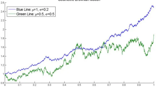
In order to understand the geometric Brownian motion, we select a graph which is based on the two sample paths of Geometric Brownian motion, with different parameters. The blue line has larger drift, the green line has larger variance.
15
Figure 3 Two sample paths of Geometric Brownian motion with different parameters. Source: From Wikimedia Commons, the free media repository
2.5 Theoretical Extensions of the Merton (1974) Model
Because the KMV model is built on the Merton model, in this section, we provide a brief review of important theoretical extensions to highlight the shortcomings of the Merton (1974) framework.
The Black and Scholes model (1973) and Merton model (1974) has built a foundation for several theoretical frameworks within credit risk analysis. The Merton (1974) model requires certain, arguably stylistic, assumptions. An often advocated shortcoming is the assumption of all debt reflected by one zero-coupon bond, oversimplifying the capital structure of companies. In general, the existing theoretical literature on structural models divides credit risk models into two branches. One branch is based on exogenous models, i.e. frameworks where the default boundary that determines when a company defaults is specified outside the model. Since the Merton (1974) model defines the default boundary outside the model through face value of outstanding debt, the model is exogenous. The other branch represents endogenous models, where default boundaries represent an optimal decision problem for management determined within the model (Imerman, 2013).
16
Nevertheless, the most important theoretical expansions follow the analytical tools provided by Merton (1974).
Longstaff and Schwartz (1995) expand the Merton (1974) introducing a first time passage framework with an exogenous and constant default boundary k, and constant recovery rates w. The first time passage feature implies that the company defaults the first time the stochastic asset process enters the time dependent k, i.e. the firm can default at any given point in time. In the standardized Merton (1974) framework, default only occurs at the specified time horizon T. The exogenous recovery rates in Longstaff and Schwartz (1995) imply that debt write-offs are dependent on the pecking order of the liability, accounting for the capital structure. Furthermore, Longstaff and Schwartz (1995) develop a two-factor framework, which is an exception from other comparable models (Dufresne and Goldstein, 2001). The two-factor framework implies that the default boundary depends on both the geometric Brownian asset motion, as well as stochastic interest rates. Interest rates follow a Markov process where they mean-revert towards a long-term level, as opposed to the standardized Merton (1974) model assuming constant short-term interest rates, implying a flat interest rate term structure. Note that both the Merton (1974) and Longstaff and Schwartz (1995) models assume that the market value of assets follow the same process, implying an increasing market value for assets over time. The default boundary is assumed to be a monotonic function of the current outstanding debt, i.e. debt remains constant over time. Thus, the leverage ratios of firms will decrease over time. This is an unrealistic assumption as empirical evidence suggests targeted leverage ratios amongst firms (Dufresne and Goldstein, 2001)
Black and Cox (1976) represent another important contribution to structural credit models. They construct a first time passage model allowing debt investors take over assets when the stochastic process enters an endogenous default boundary. Equal to Longstaff and Schwartz (1995), this creates ex ante uncertainty about the default time. Additionally, Black and Cox (1976) investigate important features often found in bond indentures. They assess safety covenants, senior/subordinated debt and restrictions concerning coupon and interest payments. All these aspects seem to affect the value of debt, thus having a significant impact on overall valuations. By combining the
17
endogenous default boundary and the role of different indentures, Black and Cox (1976) find the effects on credit spreads. While Merton (1974) determines the default boundary outside the model, Black and Cox (1976) find the optimal default boundary by maximizing the equity value (Sundersan, 2013).
In general, the reviewed models are more comprehensive than the Merton (1974) model, and pinpoint some of the weaknesses of our KMV model. Nevertheless, the Merton (1974) framework is widely acknowledged by both academicians and practitioners.
2.6 KMV model in China
Chinese empirical studies on KMV model have been focused since 2002. Cheng and Wu (2002, sample size 15), Ye, et al (2005, sample size 22), Lu, et al (2006, sample size 5) adjust the parameters of traditional KMV models and find that the mortified KMV model can timely identify and forecast the default risk of Chinese listed companies. Meanwhile, some scholars applied the KMV model to one or several industries and show that the KMV model can diversify default risk for different industries. Zhou (2009) introduced the KMV model to test credit risk for the insurance industry in China. Zhang, et al (2010) compared with 10 Chinese listed companies in Logistics with USA ones during the financial crisis and demonstrate its effectiveness of measuring credit risk. Huang, et al (2010) evaluates of default risk based on the KMV model for the three national commercial banks and also reach the same conclusion. However, all of their samples are not big enough or cover most industries.
Although previous studies have shown that KMV model is an effective tool and guidance for quantitative credit risk in China, some existing works have further discussed the modified parameters and its relationship with default probability. One of those controversial parameters is the default point. Huang and He (2010) study on probing default point of KMV in 5 listed Chinese banks and find that the model of default point differs according to different banks. However, Cheng, et al (2010) develop a novel model based on the original KMV model with tunable parameters to measure the credit risk of Chinese listed small and medium enterprise and point out that the predictive accuracy of the adjusted KMV model is stable to the change of default points. Another studied area is
18
the relationship between asset size and default. According to Moody company‟s research and Cheng, et al (2010), the asset size plays an important role in measuring default.
2.6 Classical credit risk measurement model
The development of credit risk measurement methods can be divided into three stages: First, before 1970, financial institutions basically take expert analysis, that is based on experience and subjective analysis of bank experts to assess the credit risk, the main analysis tools include 5C analysis, LAPP method, rating method, etc. Second, the end of the 1970s, financial institutions and indicators are based on credit scoring methods, such as a linear probability model, Logit model, Probit model, Altman Z- Score model and ZETA models. Third, since the 1990s, financial institutions began to use modern financial theory and mathematical tools to quantitatively assess credit risk, established a VaR-based, probability of default and expected loss of the core index measurement model, such as Credit Monitoring Model ( KMV model),which is the main methodology of the thesis. CreditMetrics model, Credit Portfolio Views, CreditMetrics + models. In this part we will briefly introduce three classical credit risk measurement methods.
2.6.1 Expert rating system
Expert rating system is a classic credit analysis method, mainly by some training after a long, rich practical experience of experts by virtue of their professional skills, personal experience, subjective judgment, and weighed against the critical factors, making a judgment of the borrower‟s probability of default, and evaluate their credit risk.
2.6.1.1 5C analysis
This is a typical analysis, through the 5C key factors to assess the borrower's credit risk: Character, investigating the borrower's reputation and past payment records. Capacity, investigating the borrower's eligibility for a loan, management ability, and profitability prospects of the project. Capital, investigating the borrower's current financial situation and how much debt assumed. Collateral, investigating the guarantor‟s financial strength and guarantee qualification, as well as the value of collateral and liquidity. Condition, investigating the economic cycle.
19
2.6.1.2 LAPP analysis
The following four aspects are also important to assess the borrower's credit risk: liquidity, through the current ratio, quick ratio and other financial ratios to investigate the borrower's capacity of assets will be converted into cash flow to repay debt. Activity, through the borrower's terms of market share and market competitiveness to investigate the operational capacity. Profitability, through the amount of the borrower's operational, profit margins of investing profitability. Potentialities, through borrower‟s product structure, management level, the business expanded to investigate the status of the development potential of the business.
2.6.2 Credit rating Models
Moody‟s, Standard and Poor's and other rating companies are specialized firms in the credit rating business. In the Moody's rating system, the highest credit rating is Aaa; followed by Aa; then in the order of credit rating from high to low is A, Baa, Ba, B and Caa, the higher the rating, the less credit risk. Standard and Poor's and Moody's rating system is similar; in the order of credit risk level from high to low is AAA, AA, A, BBB, BB, B and CCC. Afterwards, as banks and other financial institutions for the development requirements of credit rating, the two rating companies rating the credit risk of the original expansion, resulting in a finer level of risk. Standard and Poor's A rating extended to A +, A, A-, extended AA to AA +, AA, AA-, and the likes. Similarly, Moody's will expand A rating to A1, A2, A3; Aa rating will be extended to Aa1, Aa2, Aa3. In table 1, we can understand how to judge these obligations rated.
Moody‟s S&P Interpretation Moody‟s S&P Interpretation Aaa AAA Highest quality:
Extremely strong capacity. Excellent business credit. Bb1 Bb2 Bb3 BB+ BB BB- Speculative elements, substantial credit risk.
Aa1 Aa2 Aa3 AA+ AA AA-
The high quality, very strong capacity. Good business credit. B1 B2 B3 B+ B B-
Watch list credit: Speculative, high credit risk.
20 A1 A2 A3 A+ A A- Strong payment capacity. Average business credit, within normal credit standards: Caa1 Caa2 Caa3 CCC+ CCC CCC- CC Current vulnerability to default. Unacceptable business credit, normal repayment in jeopardy. Bbb1 Bbb2 Bbb3 BBB+ BBB BBB-
Moderate credit risk, medium grades, may possess certain speculative characteristics Ca C D Typically in default, with little prospect for recovery principal and interest
Table 1 Moody‟s and Standard and Poor's credit rating
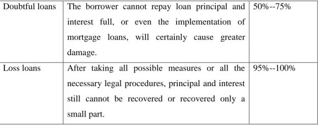
In 1998, the People's Bank of China learned the classification of loan from other countries regulatory authorities, combined with the actual situation in China, then development of "loan risk classification guidelines " improving the financial asset classification, according to different mass divided loan into five categories: Pass loans, special mention loans, subprime loans, doubtful loans and loss loans, and the last three are defective loans.
Level Definition Loss probability
Pass loans Borrower is able to fulfill the contract, have a full grasp of repaying the loan timely and full.
——
Special mention loans
Although the borrower has the ability to repay the loan principal and interest, but there are some negative factors for possible reimbursement.
5%--10%
Subprime loans The borrower's repayment ability has been impaired, cannot repay loan principal and interest rely on its normal business revenues entirely.
21
Doubtful loans The borrower cannot repay loan principal and interest full, or even the implementation of mortgage loans, will certainly cause greater damage.
50%--75%
Loss loans After taking all possible measures or all the necessary legal procedures, principal and interest still cannot be recovered or recovered only a small part.
95%--100%
Table 2 Five types‟ loans and the corresponding case in China
2.6.3 Credit Scoring Models
With respect to the importance of predicting bankruptcy of companies, many researchers have attempted to use financial ratio of companies for predicting corporate bankrupt. The typical Z-Score model and extended later to the model ZETA were introduced by Altman(1968).
Altman(1968) selected 33 bankrupt companies and 33 non-bankrupt companies as samples during the period from 1946 to 1965, Then he chooses five from the initial 22 financial ratios and adopted the companies' data before they went bankrupt, the Z-score model for the listed companies like this:
Z = 1.2X1 + 1.4X2 + 3.3X3 + 0.6X4 + 1.0X5. (2.6.1)
where
Z = overall index of the Z-score model. X1 = working capital/total assets.
X2 = retained earnings/total assets.
X3 = earnings before interest and taxes/total assets.
22
X5 = sales/total assets.
In the Z-score model, the higher the Z-score, the lower default risk. If the a company with "Z-Score" is superior to 2.99, it illustrates the firm has low default risk; if the "Z-Score" is inferior to 1.81, it illustrates the firm have high default risk; between 1.81 and 2.99, it has an indeterminate default risk.
In addition, there are Multiple Discriminant Analysis (MDA), Logistic Regression model, neural network analysis method and so on. The above mentioned various models of credit score are over-reliance on the historical financial indicators of the company, which is difficult to reflect the expected development of business in the future, the financial data having the trait of lag, poor timeliness etc. Thereby reducing the accuracy of the credit score.
23
Chapter 3
Empirical Research: Methodology and Data
3.1 The Moody’s KMV Approach
KMV model is based on the option pricing approach to credit risk as originating from Merton (1974). It was first introduced in the late 80„s by KMV1 corporation, a leading provider of quantitative credit analysis tools. The model is now maintained and developed on a continuous basis by Moody‟s KMV, a division of Moody‟s Analytics. Moody‟s Analytics acquired KMV in 2002. A large number of world financial institutions are subscribers of the model. The KMV model, however, relies on an extensive empirical testing and it is implemented using a very large proprietary database.
3.1.1 The Expected Default Frequency Credit Measure
Crosbie and Bohn (2003) presented the guidelines which are three main elements that determine the default probability of a firm:
• The market value of the firm's assets. This is a measure of the present value of the
future free cash flows produced by the firm's assets discounted back at the appropriate discount rate. This measures the firm's prospects and incorporates relevant information about the firm's industry and the economy.
• Asset Risk: The uncertainty or risk of the asset value. This is a measure of the firm's
business and industry risk. The value of the firm's assets is an estimate and is thus uncertain. As a result, the value of the firm's assets should always be understood in the context of the firm's business or asset risk.
• Leverage: The extent of the firm's contractual liabilities. Whereas the relevant measure
of the firm's assets is always their market value, the book value of liabilities relative to
1 KMV Corporation is a financial technology firm pioneering the use of structural models for credit
valuation. Founded in 1989 in San Francisco by Stephen Kealhofer, John Andrew McQuown and Oldrich Vasicek.
24
the market value of assets is the pertinent measure of the firm's leverage, since that is the amount the firm must repay.
Unlike others credit risk models, KMV does not use Moody‟s or Standard and Poor‟s statistical data to assign a probability of default which only depends on the rating of the obligor. Instead, KMV derives the actual probability of default of a given obligor, the Expected Default Frequency (EDF). The EDF is firm-specific, and can be mapped into any rating system to derive the equivalent rating of the obligor. EDFs can be viewed as a “cardinal ranking” of obligors relative to default risk, instead of the more conventional “ordinal ranking” proposed by rating agencies and which relies on letters like AAA, AA, etc. There are three key values that determine a firm‟s EDF credit measure:
• The current market value of the firm (market value of assets) • The level of the firm‟s obligations (default point)
• The vulnerability of the market value to large changes (asset volatility)
Because these are objective, non-judgmental variables, EDF credit measures have consistently outperformed the rating agencies in distinguishing between defaulting and non-defaulting firms. Not only that, they have proven to be a consistent leading indicator of agency rating upgrades and downgrades.
Among these three variables, the probability of default will increase if the current market value of the firm's assets decreases, if the amount of liabilities increases, or if the volatility of the firm's assets increases. If the market value of the firm's assets falls below the default point, then the firm defaults. Therefore, the probability of default is the probability that the asset value will fall below the default point. This is represented by the black area (EDF value) below the default point in Figure 4
25
Figure 4 Frequency distribution of a firm‟s asset value at the horizon of time H and probability of default
Source: Moody‟s KMV Analytics
The derivation of the probabilities of default proceeds in 3 stages which are discussed below:
1. Estimation of the market value and volatility of the firm‟s asset. 2. Calculation of the distance to default, an index measure of default risk.
3. Scaling of the distance to default to actual probabilities of default using a default database.
3.1.2 Estimation of the asset value and the volatility of asset return
A version of the Merton model has been adapted by Vasicek (1984) and has been applied by KMV Corporation. KMV model assumes that the company will default when the company‟s asset value is less than the liability. And it considers the value of equity as a call option, which regards asset value as the underlying asset and the debt value as the strike price. As Figure 5 shows, X represents the shareholders‟ initial investment in the26
company; D denotes the debts in default point. When the asset value more than the debt D, shareholders still gain net profits after paying debts, which is shown as an increasing equity value. The shareholders will not choose the default and the call option is exercised; when the asset value is less than the debt, shareholders transfer the total assets to creditors, which is consistent with a constant equity value. They will default and the call option is not exercised.
Figure 5 The relationship between equity value and asset value Source: Moody's KMV modeling default risk
The firm‟s asset value, Vt, is assumed to follow a standard geometric Brownian motion, i.e.:
Vt=V0exp{(µ-0.52 )t + √t Zt}. (3.1.1)
with Zt ~ N (0, 1), µ and being respectively the mean and variance of the instantaneous
rate of return on the assets of the firm, dVt=Vt2, Vt is lognormal distribution with expected
value at time t, E(Vt)= V0 exp{µt}.
If all the liabilities of the firm were traded, and marked-to-market every day, then the mission of assessing the market value of the firm‟s asset and their volatility would be straightforward. The firm‟s asset value would be simply the sum of the market values of
2The dynamics of V(t) is described by dVt/Vt =µdt+ dWt, where Wt is a standard Brownian motion, and t
27
the firm‟s liabilities, and the volatility of the asset return could be simply derived from the historical time series of the reconstituted asset value. In practice, however, only the price of equity for most public firms is directly observable, and in some cases, part of the firm‟s debt is directly traded, not all debt is traded, so that we cannot directly observe the market value of the firm. So we present two different approaches to implement the Moody‟s KMV approach.
3.1.2.1 The non-linear system of equations approach
If the market price of equity is available, the market value and volatility of assets can be determined directly using a Black-Scholes-Merton (BSM) options pricing based approach. In order to make the model tractable, KMV assumes that the capital structure is only composed of equity, short-term debt, which is considered equivalent to cash, long-term debt which is assumed to be a perpetual, and convertible preferred shares3. With these simplifying assumptions, it is then possible to derive analytical solutions for the value of equity Et, and its volatility, E:
Et = Vt N ( 1) –X e rτ N ( 2) (3.1.2)
In which 1 and 2 are respectively given by :
( )
√ (3.1.3a)
√ (3.1.3b) where
Et: the equity‟s market value;
X: the liabilities‟ book value;
Vt: assets‟ market value;
τ: maturity;
r: risk-free interest rate;
3 In the general case the resolution of this model may require the implementation of complex numerical
techniques, with no analytical solution, due to the complexity of the boundary conditions attached to the various liabilities. See, for example, Vasicek (1997).
28
σA: the underlying asset‟s volatility;
N ( i): the normal distribution‟s cumulative probability function.
In addition the volatility of the underlying assets‟ value (σA) has such relation with the
volatility of the equity‟s market value(σE):
N ( 1) (Vt / Et) . (3.1.4)
Because the market value of equity is observable and the equity volatility can be estimated, so we can use the equation (3.1.2) and equation (3.1.4) to determine the time-t value of assets Vt and volatility V that are implied by the current equity value, equity
volatility, and capital structure. For example, Jones et al. (1984) and Ogden (1987) use this non-linear system of equations approach for estimating the asset volatility. Still, the solution to this system of equations is non-trivial since 1 and 2 depend both on the two
unknown quantities, i.e. asset value Vt and volatility σV. Even though a numerical
solution is required, this can be easily performed (e.g. In Excel or Matlab) using a routine based on the Newton-Raphson algorithm4.
However, most of the empirical studies argue that “the relationship between 𝐸 and v
from the equation(3.1.4) holds only instantaneously, for instance, Crosbie and Bohn (2003), Vassalou and Xing (2004), Patel and Vlamis (2007), Bharath and Shumway (2008), and ect, and in practice, the market leverage moves around far too much for equation(3.1.4) to provide reasonable results”. To solve the problem, an iterative procedure is usually introduced as follows.
3.1.2.2 The iterative approach
In order to calculate the asset volatility v, generally we use the iterative approach
proposed by Crosbie and Bohn (2003) and Vassalou and Xing (2004)5. This approach is a relatively recent technique of getting asset value and asset volatility and has presented very useful for predicting default probability.
4 This algorithm is first in the class of Householder's methods, succeeded by Halley's method. The method
can also be extended to complex functions and to systems of equations. 5
29
In general, we would like to implement the Moody‟s KMV model with a one year horizon that is our purpose would be to estimate the default probability in one year. To accomplish this task we need to estimate the asset value and volatility. The iterative procedure to estimate such unobservable variables is as follows:
1. Define a given tolerance level for convergence.6
2. According to the Vassalou and Xing (2004, Page 835), we will use daily data from the past 12 months (252 trading days) to obtain an estimate of the (historical) equity volatility E , which is used as a starting value for estimating V. Besides,
we may create a vector of asset prices Vt−a, for a = 0, 1, ..., 252. The asset valueis
regarded as the sum of the market value of equity Et−a and the book value of
liabilities Dt−a. The market value of equity is typically regarded as market
capitalization and the book value of liabilities as debt in one year plus half the long-term debt. Then, set the initial value for the estimation of σv, V as the standard deviation of the log asset returns computed with the Vt−a vector.
3. Rearranging the Black and Scholes (1973) equity-pricing equation for the asset value of the firm, we obtain
Vt = Et + X e rτ N ( 2) / N ( 1) . (3.1.5)
We use this formula for each trading day of the past 12 months, compute the asset value Vt−a using Et−a as the market value of equity and Xt−a as the book
value of the firm's liabilities of each day t − a, that has maturity equal to T. By doing this, we obtain daily values for Vt−a. This system of equations is composed
by 253 equations with 253 unknowns.
4. This step is to compute the standard deviation of this new Vt−a vector, which is
then used as the value of σV for the next iteration.
6
30
5. Repeat this procedure until the values of σV from two consecutive iterations
converge.
For most firms, only a few iterations are necessary for σV to converge. Once this value is
obtained, we may easily retrieve the asset value Vt through equation (4.5). Moreover,
once daily values of Vt−a are estimated, we can compute the drift µ, by calculating the
mean of the log asset returns of the final Vt−a vector.
3.1.3 Calculate the Distance-to-default
KMV implements an intermediate phase before computing the probabilities of default, which is called “Distance-to-Default (DD).” DD is the number of standard deviations between the mean of the distribution of the asset value and a critical threshold, the “default point (DPT)”. The DPT is defined in Crosbie (2003) as half the long-term debt(LTD) plus the par value of current liabilities, including short-term debt (STD), which is an attempt to capture the idea that short-term debt requires a repayment of the principle soon whereas long-term debt requires only coupon payments to be met.
DPT :=STD+0.5LTD. (3.1.6) Consequently, the distance-to-default (DD) is given by
(3.1.7) This measures the distance-to-default in terms of the standard deviation of the assets. Notice that this measure combines three key credit issues: the market value of the firm's assets, its business and industry risk, and its leverage.
In the current Moody‟s KMV model the distance – to – default is computed as ( )
√ (3.1.8)
In this equation Payouts reflect the asset drainage through cash flows until T (i.e. debt coupons and preferred and common dividends), and µ is the expected growth rate of the
31
assets which is typically hard to estimate. One possibility is to use a unique µ per sector or industry, which would be easier to estimate.
3.1.4 Compute the probability of default
The last phase consists of mapping the DD to the actual probabilities of default (DP), for a given time horizon. These probabilities are called by KMV, for Expected Default Frequencies (EDF).
Moody‟s KMV obtains the relationship between distance-to-default and default probability from data on historical default and bankruptcy frequencies. Their database includes over 250,000 company-years of data and over 4,700 incidents of default or bankruptcy. From this data, a lookup or frequency table can be generated which relates the likelihood of default to various levels of distance-to-default.
3.1.5 Advantage of the Moody’s KMV model
There are four main advantages which led this model widely used in the areas of credit risk assessment and the forecasting of financial distress.
1. The KMV model is superior to the timeliness of the assessment models. The KMV model uses the real-time data. It can update the probability of default in real time based on the data on the securities market.
2. The assumption of KMV model is weak. The efficient market assumption is not required. This is very applicable in the weak effective securities market of China. 3. The KMV model is a forward-looking method. The data used in the model
reflects the expected value of the company and the judgment of the company‟s future development trends of the investors.
4. The KMV model is a base method which is different from the ordinal method. It can not only reflect the credit risk level of the order, but also reflect the credit risk level of the degree of difference.
32
3.2 Selection of parameter
Equity value ( Et )
The equality value is equal to the annual market value of equity. Since this study chooses the data window after 2006 in which china‟s split share reform took effect, it doesn't contain any further calculation with the classification of sharable equity value and non-shareable equity value7. In this paper, Data is obtained directly from RESSET Solution Database.
Book Value of Liability(X)
The short-term debt (STD) plus the long-term debt (LTD) is the total liability.
X:=STD+LTD (3.2.1)
Equity value volatility (σE )
In this paper, The volatility of equity value is calculated from the historical daily equity return data. We assume that the price of the shares obeys logarithmic normal distribution. Thus the volatility of equity value is expressed as ( Li and Zhang, 2010):
√ ∑ ( ̅ ) (3.2.2)
(3.2.3)
where denotes the log return at time m; means the closing price of i day; m is the trading day, which is approximately equal to 252 days. Excel software is use for the above calculation.
Maturity( τ )
We set the calculation time of default distance in one year (τ =1 ) .
7 Before Chinese government has taken stock equity reform from 2006. Due to the special of the
development of Chinese stock market, shares of listed companies is artificially divided into two parts, the non-tradable shares and tradable shares,