Modelling the polymeric profile extrusion cooling stage with OpenFOAM®

João Manuel Duarte Ferreira

Modelling the Polymeric Profile

Extrusion Cooling Stage with OpenFOAM®

João Manuel Duarte Ferreira

Modelling t he P ol ymer ic Pr ofile Extr usion Cooling St ag e wit h OpenF O AM®

Universidade do Minho

Escola de Engenharia

Dissertação de Mestrado

Ciclo de Estudos Integrados Conducentes ao

Grau de Mestre em Engenharia de Polímeros

Trabalho efectuado sob a orientação do

Professor Doutor João Miguel Amorim Novais Costa

Nóbrega

João Manuel Duarte Ferreira

Modelling the Polymeric Profile

Extrusion Cooling Stage with OpenFOAM®

Universidade do Minho

ACKNOWLEDGMENTS

During this journey of project development and writing this thesis, several persons were fundamental to accomplish my objectives.

Firstly, I would like to thank Professor João Miguel Amorim Novais Costa Nóbrega for all the guidance, corrections and knowledge inputs. Also, for all the opportunities I had access during this journey.

I also would like to thank to all the members of Gompute S. L. company, that provided crucial help throughout the development of this work.

Finally, I am forever thankful to my parents and my brother for all the support, help and guidance through these years.

ABSTRACT

Nowadays the importance of the Computational Fluid Dynamics in polymer processing applications is really high, since it can provide useful data that can be used to anticipate the behaviour of the system under study, when subjected different service conditions, and thus guide its design and/or optimization. There are different options available when choosing the platform to perform such studies, which can be mainly divided into commercial and the free/open source numerical codes. Besides the obvious differences in terms of cost, the first do not allow changes on the source code while the latter allows it. OpenFOAM® computational library is an example of a free and open source code that comprises several pre-programmed solvers, allows full customization by the user and provides a solid and consolidated base for the development of customized numerical tools.

The problem of interest integrated in the field of polymer processing, comprises the modelling of cooling and calibration of an extruded polymer profile with unstructured meshes. Numerical tools had to be created to fulfil the requirements and for that OpenFOAM® was used and modified.

To meet the modelling requirements the cthMultiRegionFoam solver, that solves momentum, energy and continuity equations, was modified to solve only the energy conservation equation since, at the profile extrusion calibration stage, the velocity field is known and constant on the entire domain. Different verifications were performed on the developed code, by comparing its predictions with, analytical solutions, for simple problems and with results available on the scientific literature, in order to evaluate its accuracy. Convergence order studies were performed using different meshes to evaluate the order of convergence and the calculation accuracy and to choose the best mesh refinement level to use on the subsequent studies. In order to evaluate the code capabilities, studies involving cooling and calibration of an extruded polymer profile using different layouts, process and geometrical parameters were also undertaken.

The developed code was tested under different verification problems and, the results obtained, allowed to assess it, for the cooling stage. Regarding conclusions, the studies made possible the evaluation of which process and geometrical parameters influence the most. This revealed that using several calibrators have advantages when compared to only use one, also that the profile velocity has the higher impact on the final results.

RESUMO

Hoje em dia, é grande a importância da Dinâmica de Fluídos Computacional nas aplicações de processamento de polímeros, a informação produzida por estes estudos possibilita a antecipação do comportamento que o sistema em estudo terá, quando sujeito a diferentes condições de serviço, e ajudar no desenho e otimização do mesmo. Existem diferentes opções disponíveis para a execução deste tipo de estudos, que podem ser divididas em códigos comercial e gratuito/aberto. À parte da diferença óbvia em termos de custo, o primeiro não possibilita a alteração do código fonte, enquanto o segundo o possibilita. OpenFOAM® é um exemplo de código aberto e gratuito, que contém diversos solvers pré-programados, possibilita a sua total modificação por parte do utilizador e apresenta-se como um base sólida e consolidada para o desenvolvimento de ferramentas numéricas personalizadas.

O problema de interesse integrado na área de processamento de polímeros, compreende a modelação da etapa de arrefecimento e calibração do processo de extrusão de perfil, utilizando malhas não estruturadas. Ferramentas numéricas tiveram de ser desenvolvidas para cumprir os requisitos de modelação e, para isso, o OpenFOAM® foi utilizado e modificado.

Para cumprir os requisitos de modelação o solver chtMultiRegionFoam, que resolve as equações de momento, conservação de energia e continuidade, foi modificado para apenas resolver a equação de conservação de energia, dado que na etapa de calibração da extrusão de perfil, o campo de velocidades é conhecido e constante em todo o domínio. Diferentes verificações foram realizadas com o código desenvolvido, comparando as suas previsões com soluções analíticas, para problemas simples e com resultados disponíveis na literatura científica, para avaliar a sua precisão. Estudos de ordem de convergência foram realizados com diferentes malhas para avaliar a convergência e a precisão de cálculo, de forma a também escolher o melhor refinamento de malha para os estudos a realizar. Para avaliar as capacidades do código, estudos envolvendo a etapa de arrefecimento e calibração da extrusão de perfil com diferentes layouts, parâmetros geométricos e de processo foram realizados.

O código desenvolvido foi testado sobre diferentes problemas de verificação e, com os resultados obtidos, possibilitou a sua aferição para a etapa de arrefecimento. Relativamente a conclusões, os estudos possibilitaram a avaliação de quais os parâmetros geométricos e de processo têm mais influencia. Isto relevou que a utilização de diversos calibradores tem vantagens à utilização de apenas um e também que a velocidade do perfil é o parâmetro com mais impacto nos resultados finais.

C

Acknowledgments ... iii

Abstract... v

Resumo... vii

List of Figures ... xi

List of Tables ... xiii

List of abbreviations and acronyms ... xv

1. Introduction ... 1

1.1 Problem to be solved ... 1

1.2 State of the art ... 2

1.3 Objectives ... 4

1.4 Thesis structure ... 4

2. Numerical code ... 5

2.1 OpenFOAM Computational Library ... 5

2.2 Solver chtMultiRegionFoam ... 6

2.3 Numerical Procedure... 8

2.4 Code Modifications Performed ... 11

3. Numerical Code Verification ... 13

3.1 Verification 1 – “Two Rectangular Slabs” ... 13

3.1.1 Computational Model ... 15

3.1.2 Results and Discussion ... 17

3.2 Verification 2 – “Complex Layout” ... 21

3.2.1 Computational Model ... 22

3.2.2 Results and Discussion ... 23

4. Polymer Calibration Case Study... 27

4.1 Three Calibrators Layout ... 29

4.2 One Calibrator Layout ... 31

4.3 Process and Geometrical Parameters ... 33

4.4 Mesh Sensitivity Study ... 34

x

4.6 Effects of the Geometrical and Process Parameters ... 42

5. Conclusions and Outlook ... 47

5.1 Conclusions ... 47

5.2 Outlook ... 48

LIST OF FIGURES

Fig. 1 - Typical extrusion line for the production of thermoplastic profiles, Nóbrega J. M. et al. (2004) . 1 Fig. 2 - Flowchart of chtMultiRegionFoam solver steps ... 6 Fig. 3 - Flowchart of the modified solver steps ... 11 Fig. 4 – Verification 1 case study: geometry and boundary conditions, Nóbrega J. M. et al. (2004) .... 14 Fig. 5 – Verification 1 case study mesh M5 ... 16 Fig. 6 – Analytical and numerical results for the temperature distribution of the Verification 1 case study: perfect contact ... 17 Fig. 7 – Temperature [ºC] distribution for the perfect contact interface, calculated by the developed code with M5 ... 18 Fig. 8 – Analytical and numerical results for the temperature distribution of the Verification 1 case study: contact resistance ... 19 Fig. 9 – Temperature [ºC] distribution for the contact resistance interface, calculated by the developed code with M5 ... 20 Fig. 10 - "Complex Layout" geometry and boundary conditions, dimensions in mm. Nóbrega J. M. et al. (2004) ... 21 Fig. 11 – Verification 2 case study mesh M6 ... 23 Fig. 12 - Results for several meshes on the location 7/50 of the complex layout, benchmark from Nóbrega J. M. et al. (2004) ... 24 Fig. 13 - Temperature distribution illustration for the Verification 2, with M6 ... 25 Fig. 14 - Temperature distribution for the Complex Layout case study, with M6. Benchmark from Nóbrega J. M. et al. (2004) ... 26 Fig. 15 - Polymer/calibrator cross section (dimensions in mm), Nóbrega J. M. et al. (2004) ... 27 Fig. 16 - Geometry of the three calibrator layout (dimensions in mm), Nóbrega J. M. et al. (2004) .... 30 Fig. 17 – Three calibrator case study mesh ... 31 Fig. 18 - Geometry of the one calibrator layout (dimensions in mm), Nóbrega J. M. et al. (2004)... 31 Fig. 19 - One calibrator case study mesh ... 32 Fig. 20 - Temperature [ºC] distribution illustration for the three calibrator layout, reference case c1 .. 37 Fig. 21 - Temperature [ºC] distribution illustration for the one calibrator layout ... 40

LIST OF TABLES

Table 1 - Convergence order for perfect contact results of the Verification 1 case study ... 18

Table 2 - Convergence order for resistance contact results of the Verification 1 case study ... 20

Table 3 – L2 errors and convergence order for the complex layout on the locations z/L = 7/50, 30/50 and 50/50 ... 24

Table 4 - Conditions and Properties used on the studies, Nóbrega J. M. et al. (2004) ... 28

Table 5 - Different conditions for outer surfaces and interface polymer/calibrator, Nóbrega J. M. et al. (2004) ... 29

Table 6 - Process and geometrical parameters used ... 34

Table 7 - Results and convergence order for the three calibrator layout, case c0 ... 35

Table 8 - Heat Fluxes [W] through boundaries of the three calibrator layout study ... 36

Table 9 - Temperatures at the end of the profile cross section, three calibrator layout ... 39

Table 10 - Heat Fluxes [W] through the boundaries for the table 5 cases, one calibrator layout ... 40

Table 11 - Temperatures at the end of the polymer profile cross section, one calibrator layout ... 41 Table 12 - Temperatures and total heat removed for the process and geometrical parameters studies 43

LIST OF ABBREVIATIONS AND ACRONYMS

OF - Open Source Field Operation and Manipulation, OpenFOAM® CFD – Computational Fluid Dynamics

HPC – High Performance Computing FEM – Finite Element Method FVM – Finite Volume Method

1.

INTRODUCTION

1.1 Problem to be solved

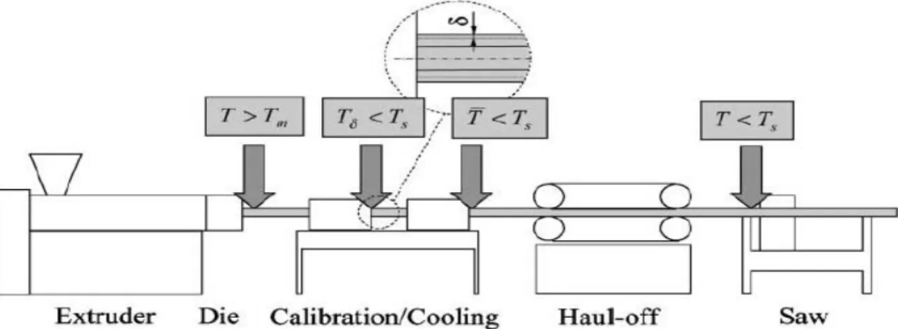
The problem of interest in this work is the modelling of the cooling and calibration stage of a thermoplastic profile extrusion line. A profile extrusion line is typically composed by five stages, as illustrated in the Fig. 1, which can be described as follows:

1) Extruder – At this stage the raw polymer pellets are melted, homogenized and conveyed, with the help of a screw, into the extrusion die;

2) Die – The forming stage, where the polymer melt is progressively transformed from the circular cross section, at the extruder outlet, to a cross section similar to the profile to be produced;

3) Calibration/Cooling – The polymer melt is cooled down, and also calibrated, until a sufficiently low temperature that guarantees its shape during the remaining stages of the extrusion line;

4) Haul-off – This is a device that pulls the extrudate and is responsible for the maintenance of the extrusion linear velocity;

5) Saw – At final stage of the process the extrudate is cut into smaller sections and stored;

Due to the complex rheological behaviour of polymer melts, it is difficult to obtain a profile with the desire cross section after emerging from the extrusion die flow channel. Thus the third stage of the

2

process, is very important, not only to impose the profile main dimensions, but also to assure enough mechanical resistance to support the loads imposed at the downstream stages. Being a relevant stage for the extrusion process makes the numerical modelling of this stage quite relevant.

The numerical modelling of the calibration/cooling stage provides a high quantity of useful information that can be used to improve the system efficiency, leading to higher production rates or to achieve a more uniform cooling, relevant to minimize the level of induced thermal residual stresses. The reasons behind the modelling of this stage are the need to obtain the temperature distribution on the polymer profile. The more uniform temperature distribution along the profile the better and this can be obtained by adjusting the geometrical and process parameters on the calibrator, such adjustments can be performed considering the information retrieved from the numerical modelling studies. At the end, studying the influence of the parameters that can be controlled on this stage, it is possible to obtain the most efficient system layout.

The extrusion cooling stage comprises two main components (see Fig. 1). A polymeric profile, produced by extrusion, and a metal calibrator. The polymer profile travels at a constant and uniform velocity relatively to the calibrator, which is stationary. Regarding the calibrator, comprises a variable number of cooling channels, which are filled with a cooling fluid at low temperature that are used to remove energy from the system. Depending of the cooling requirements more than one calibrator can be used.

This stage has variables that can be changed or controlled. In terms to conceive a calibration system one must specify: the number of cooling units, their length and distance between them. Additionally, the variables of the process that can be controlled are: the cooling fluid temperature and the profile velocity. These are the main variables of the process that can be controlled and/or changed and that can be established with the support of numerical studies.

1.2 State of the art

The use of CFD on the polymer processing area is growing at a good rate, which is logic since the advantages of using numerical modelling tools, during the design stage, are immense. For areas like injection moulding, CFD is used frequently while to design parts and/or their processing tools, although on the extrusion process, CFD is not used so frequently, mainly due to the absence of adequate numerical tools, which is a clear limitation for the extrusion process development.

The first works available in the literature was the 2D FEM approach proposed by Menges et al. (1987), which was able to deal with any profile cross section but without considering axial heat fluxes. Later, an approach named Corrected Slice Method was proposed by Sheehy et al. (1994). This extends the 2D approach described by Menges et al. (1987), to take into account the axial heat fluxes within the system. The developed method allow the use of complex cross sections considering axial heat fluxes, although with the restrain of being an hybrid 2D model, which limits, in several ways, the extent of the studies that can be conducted. A more complex approach was handled by Nóbrega J. M. (2004), where numerical tools were developed to model this stage, and were coupled with automatic optimization approaches. In the same subject, another approach was proposed by Nóbrega J. M. et al. (2004) to model the thermal interchanges between the polymer profile and the calibrator. In this study the temperature distribution of the polymer profile when crossing this stage was obtained, allowing to predict the efficiency of the cooling system. Despite their obvious advantages, these numerical tools can only work with structured meshes which restrain, in a significant way, the complexity of the profile cross sections that can be studied.

It is important to understand that the development of numerical tools need a large amount of information about the specific situation intended to be modelled, such as the properties of the material that are being used on the model. Regarding the cooling and calibration stage of the extrusion process, the interface between the polymer and the calibrator is a critical area of the system, which requires special techniques to obtain the heat transfer coefficient, in order to correctly consider the heat exchange between both parts. The characterization of the heat transfer coefficient for the extrusion cooling system was conducted by Pittman J. F. T. et al. (1994) and Mousseay P. et al. (2009) where the contact resistance is evaluated. The first study is the most complete one, although this provides useful information just for thick pipe extrusion where the cooling is performed by immersion in water. This is not the usual approach on profile extrusion, where the cooling is performed by contact between the profile and the calibrator, which affects the heat transfer at the polymer-calibrator interface and creates problems related with friction. The second study allows the understanding of all the heat transfer phenomena occurring during the profile cooling stage, although the analysis were undertaken applying vacuum on both side of the plastic tape, which usually is not the case in practical extrusion. Both studies provide useful information, regarding the evaluation of the heat transfer coefficient on the polymer-calibrator interface, however the values obtained are for specific conditions. Recently, a prototype developed by Carneiro O. S. et al. (2013) to perform an evaluation of the heat transfer coefficient value on the interface polymer-calibrator, under the typical conditions used on the profile extrusion.

4

The information available in the scientific literature show that is possible to correctly model the cooling and calibration stage of the extrusion process and that there are tools already developed capable of modelling it, although, with some limitations. More versatile numerical codes, able to deal with realistic problems, which in general involve complex geometries, are needed. To be able to deal with more complex geometries, these numerical tools should be able to work with 3D unstructured meshes.

1.3 Objectives

The main objective of this work is to develop and verify numerical tools adequate to aid the design of the cooling and calibration stage of profile extrusion comprising complex problems.

Several smaller tasks have to be fulfilled to reach the main purpose stated above. At the initial part of the work a numerical code must be developed to meet the modelling requirements of the cooling stage of profile extrusion and also be able to deal with complex geometries, thus it should work with unstructured meshes. The second target of this work is the developed code verification. For this purpose, the developed code predictions should be compared with analytical results, for simple problems, with results provided in the literature. During the verification work, the order of convergence of the developed code should be also verified. It is also an objective of this work to perform systematic studies with a typical profile extrusion problem, to evaluate the developed code sensitivity and, in a qualitative manner, its predictions.

1.4 Thesis structure

The Section 1 briefly describes the polymer extrusion process and addresses the problem being solved in this project, as well as a state of the art, that summarizes the most relevant contributions on the area. The Section 2 presents the work undertaken to develop the numerical code, adequate for the problem of interest. The Section 3 comprises the code verification, which was done using two different case studies. Following, on Section 4, aiming to evaluate the sensitivity of the developed code, it was used to investigate, in detail, the cooling stage of a representative profile extrusion problem. The Section 5, and final one, presents the conclusions and outlook of the work done in this project.

2. NUMERICAL CODE

2.1 OpenFOAM Computational Library

Open Source Field Operation and Manipulation, abbreviated as OpenFOAM®, is a free and open source C++ numerical computational library. It is used primarily to create executables, known as applications, this category is then divided into two sub-categories which are solvers, routines used to solve continuum mechanics problems, using the Finite Volume Method (FVM), and utilities which are used to all types of data manipulation from pre-processing to post-processing. A large amount of solvers and utilities are available in each OF distribution, covering a large range of problems. Also OF has its own pre- and post-processing environments as well as the solving one, this means that the all main steps of a numerical study are done under OF’s utilities which ensures correct data travel between the environments. Although the main strength of OF is that solvers and utilities can be created or modified by the users and then be used on a specific case, this requires some knowledge of the underlying method, physics and also programming techniques involved. Bottom line the OF provides a solid and verified base to produce numerical tools to solve specific problems, allowing the user to add desired features to applications or utilities or even remove some to obtain better performance.

As stated above one of the main advantages and capabilities of OF is the free and open source nature of the code, allowing to understand, from the user perspective, how the routines are performed and use them without any type of fee. Another main advantage is allowing the user to modify the source code of the already provided applications or utilities and also provide a solid base to make new applications or utilities without any kind of restrain, this opens a whole new level of possible developed work. The nature of the code also allows the users to exchange knowledge and creations which makes this library very community driven and a lot of improvements are inserted in every new version release. With this the number of applications is large making possible a huge amount of different CFD studies using this library.

The need to develop numerical tools to solve the problem addressed in this project made OF a seriously interesting base to work. In fact, OF has a solver that almost meets all the requirements to solve the problem of interest, although a few changes on it were needed to make it suit the modelling requirements. Also, the OF is booming in several CFD areas, although there are just a few studies on the

6

polymer extrusion, then here OF is going to be tested to model the extrusion process calibration and cooling stage. The capability of OF to efficiently work in an HPC environment is also a good reason to work with it in this project, since an HPC platform was available to perform the studies. Using this HPC platform, that provides a higher amount of resources, it reduces the calculation time as well as allow the use of bigger meshes.

2.2 Solver chtMultiRegionFoam

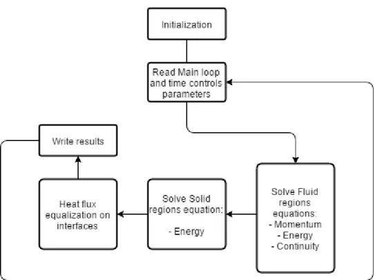
The OF chtMultiRegionFoam is a solver developed for conjugate heat transfer between solid and fluid regions. The differences between the type of regions, considered by the solver, are that a solid region is stationary, where the energy conservation equation is solved, and a fluid region has a velocity field, where the linear momentum, energy conservation and continuity equations are solved. The solvers flowchart is illustrated in Fig. 2.

The solver performs several steps during, which can be described as follows:

1) Initialization – This step starts by initializing the turbulence, radiation and thermodynamic models and the time variables. Then it continues with the definition of the solid and fluid regions on the mesh, finalizing with the creation of the fields present in each region like velocity, pressure and temperature;

2) Read Main loop and time controls parameters – In this step the solver reads the control parameters that are used by the Main loop algorithm and by the solver;

3) Solve Fluid regions equations – For each fluid region the momentum, energy conservation and continuity equations are solved;

4) Solve Solid regions equations – For each solid region the energy conservation equation is solved;

5) Heat flux equalization on interfaces – In this step the heat flux is calculated on the interfaces in preparation for the next time step to account the heat transfer between different regions;

6) Write results – the results obtained by solving the fluid and solid regions equations are written and the solver goes back to the step 2 to solve the equations for the next time step;

Analysing the model requirements, as described on the Section 1.1, and the potential of chtMultiRegionFoam it can be concluded that this solver can be used to solve the problem being addressed in this project. With the capability of solving the equations on two or more different regions, with different properties but connected by one or more boundaries, makes it a good choice, when dealing with a model that has at least two different regions, polymer and calibrator.

8

2.3 Numerical Procedure

The model being developed here requires that only the energy conservation equation needs to be solved to obtain the thermal field on the calibrator (2) and polymeric profile (1) regions. This happens because the velocity field on the profile is known and also constant throughout the entire domain, which makes the energy conservation equation the only one that has to be solved. As described by Nóbrega J. M. et al. (2004), the energy conservation equation can written as follows for the polymeric profile:

∇ ∙ (𝜌𝑐𝑝𝑢⃑ 𝑇) −

𝑘 𝜌𝑐𝑝

∇2𝑇 = 0 (1)

and for the calibrator:

𝑘 𝜌𝑐𝑝

∇2_{𝑇 = 0} (2)

The polymer region have two different transport mechanism, which are the advection and diffusion. For the calibrator region, where the velocity field is null, which makes the only transport mechanism existent in this region be the diffusion.

The system to model two different regions where the equations described above are solved. To account the heat fluxes exchanged between these two regions, the interface boundary condition must be given. This interface boundary condition can be treated in two different ways, in one hand it can be perfect contact interface (4), this assumes both temperature and heat flux continuity, and on the other hand a contact resistance (5) that assumes the existence of a temperature discontinuity at the interface. Based on the above, this interface boundary condition can be modelled mathematically by the following equations: (𝑇_𝑝 = 𝑇_𝑐)interface (3) 𝑘_𝑐(𝜕𝑇𝑐 𝜕𝑛)interface= −𝑘𝑝( 𝜕𝑇𝑝 𝜕𝑛)interface (4)

for the prefect contact interface, 𝑘𝑐( 𝜕𝑇_𝑐 𝜕𝑛)interface= −𝑘𝑝( 𝜕𝑇𝑝 𝜕𝑛)interface= ℎ𝑖(𝑇𝑝− 𝑇𝑐)interface (5)

for the contact resistance interface. In these equations in terms of notation, ℎ𝑖is the interface heat transfer

coefficient and 𝑛 is the interface normal vector.

The Equation (6) represents the energy equation used by the OF.

𝜕𝜌𝑐𝑝𝑇

𝜕𝑡 + ∇ ∙ (𝜌𝑐𝑝𝑢⃑ 𝑇) − 𝑘 𝜌𝑐_𝑝∇

2_{𝑇 = 0} (6)

This form of energy conservation equation contains the rate of change, advection and diffusion terms. Since the problem of interest is steady state, the rate of change term does not have to be considered, however it was used in the numerical calculations just for relaxation purposes, to facilitate the convergence. Accordingly all the results were considered when the calculations achieved steady state conditions. This was done by checking, in each time step, the initial and final residual values of the equation. When, for several time steps, these values were the same and do not changed, the steady state was assumed.

The Equations (1) and (2) are simplifications of Equation (6). For the polymer, Equation (1), the diffusion term is expanded for all directions and the advection term is only expanded for the z direction, since only the z velocity component is not null. In the case of the calibrator region, Equation (2), since it is stationary, the only term that subsists is the one that accounts for the contribution of heat diffusion.

Numerically all the governing equation terms have to be discretized. The schemes employed in this operation will have a direct influence on the order of convergence of the numerical code. The advection, diffusion and rate of change terms were discretized using, respectively, bounded Gauss upwind, Gauss linear uncorrected and Euler schemes. The schemes used to discretize both, the diffusion and advection terms, are second order, while for the rate of change is first order. However, since the

10

relevant results will be the ones of the steady state conditions, this first order scheme, will not influence the order of convergence for the developed code.

Another important subject regarding the numerical procedure is the type of boundaries and boundary conditions used on the model. Being the model composed by two different regions, polymer and calibrator, and the equations solved for each one of the regions, an interface between the two regions is part of it, meaning that a boundary has to be modelled to consider that interface.

In terms of the type of boundary used to model the interface between the regions, the mappedWall type was used. This type of boundary is used to couple two boundaries from two different regions, this means that the new boundary allows exchange of data between the regions, usually a field depending on the boundary condition used (OpenFOAM® Thermal modelling, 2014). This boundary type works by obtaining the values present on the interface boundary faces of the other region and use them on the calculations on its own region, creating a connection and allowing the exchange of energy, for example, between the regions.

Regarding the boundary condition applied on the interface between the regions, the compressible::turbulentTemperatureCoupledBaffleMixed condition was used. This boundary condition was designed to couple thermally solid and fluid regions, meaning that heat fluxes can be exchanged between both regions (OpenFOAM® Thermal modelling, 2014). It allows the user to introduce thermal layers on each side of the interface, each layer defined by its thickness and thermal conductivity, to create a contact resistance, see Eq. (5), between the regions. This boundary condition also allows to model the interface as perfect contact, see Eq. (4), if none thermal layer is defined. The properties of these layers are obtained using the relation ℎ = 𝑘𝑙

𝑡𝑙

⁄ , where h is the contact resistance, k the thermal conductivity and t the thickness of the layer. The procedure to model an interface with a certain value for the contact resistance is the definition of the thickness by the user, and, using the previous relation, calculate the thermal conductivity. Subsequently, the values of thickness and thermal conductivity, are inserted at the interface boundary condition in both regions. On the boundary of each region used to thermally couple the regions, the same entries have to be used in each one of them, which creates two thermal layers with the same thickness and thermal conductivity.

Considering the model being developed in this project this boundary condition meets all the requirements to the construction of the interface between the polymer and calibrator.

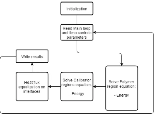
2.4 Code Modifications Performed

Despite the fact of being a good choice to model the problem of interest, chtMultiRegionFoam, described on the section 2.2, it is not fully ready to be applied, some simplifications had to be performed on the solver source to solve only the required governing equations presented in Section 2.3. As illustrated on Fig. 2 on the fluid (polymer) region the solver calculates three different equations, while for the case of interest only the energy conservation equation has to be solved in this regions. In the polymer regions the velocity is known a priori and has a constant value.

The flowchart of the simplified solver is presented in Fig. 3.

The flowchart of the new solver, illustrated on Fig. 3, is similar to the one illustrated by the Fig.2, although some changes were implemented. The step Solve Fluid regions equations is now smaller and the number of equations that are solved here was reduced. The momentum and continuity equations were removed from the source code, making the modified solver to use only the energy conservation when solving the equations for the polymer regions.

These simplifications were implemented on the original source code files, to create a new solver adequate to calculate the temperature distribution for the profile extrusion calibration/cooling stage.

3. N

UMERICAL CODE VERIFICATION

In this chapter the previous developed code is going to be verified, which two problems comprising different complexity levels. The first verification consists of two stationary rectangular slabs that share a common face. The second verification consists in a more complex layout composed by a moving polymer sheet that is cooled by calibrator containing three transverse cooling channels.

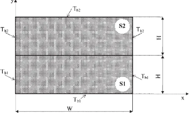
3.1 Verification 1 – “Two Rectangular Slabs”

The two rectangular slabs case study, illustrated in Fig. 4. The two slabs made by different material share a common face. The boundary conditions used on the outer walls are fixed values of temperature, which is different in each slab.

The verification is going to be performed with comparison of the analytical solution for this problem, as described by Nóbrega J. M. et al. (2004), with the results for the temperature distribution obtained with the developed code considering the two possible interfaces, perfect contact and contact resistance. A convergence order study using several meshes, with different refinement levels, is also performed to evaluate the order of convergence of the developed code.

In terms of procedure, to obtain the geometries, this starts by being a single region which later is split into the desired two regions. This procedure is used due to the fact that the solver works with mesh regions and, to obtain these mesh regions, the entire geometry was constructed and meshed in a whole, which then was split into the different regions. The mesh used in this verification was obtained using blockMesh (“Mesh generation with blockMesh”, 2015), a mesh generation utility supplied with OF. With this the mesh for the entire geometry was created and after, using the topoSet (“topoSet”, 2012) utility, was divided into the S1 and S2 regions.

In terms of converge order study, this was performed with a mesh refinement ratio of 2, the error L-Infinty, L∞, which is defined as: ‖𝑥‖_∞= 𝑚𝑎𝑥_𝑖|𝑥𝑖| where 𝑥 is difference between the numerical and

the analytical value at the same location. The convergence order was calculated using 𝑜𝑟𝑑 = ln ( 𝑒𝑟𝑟𝑜𝑟(𝑀𝑖)

𝑒𝑟𝑟𝑜𝑟(𝑀𝑖+1)) ln ( 𝐿𝑀_𝑖+1

𝐿𝑀_𝑖 )

⁄ , being LM_i and LM_i+1 the edge length of two meshes with different refinement

14

Fig. 4 – Verification 1 case study: geometry and boundary conditions, Nóbrega J. M. et al. (2004)

The analytical solution for this problem is given by Nóbrega J. M. et al. (2004) and for the case of perfect contact interface is given by:

𝑇 = 𝑇_𝑏1+ ∑2 𝜋(𝑇𝑏2− 𝑇𝑏1) (−1)𝑛+1 𝑛 ∞ 𝑛=1 𝑘₂ (𝑘₂+ 𝑘₁)sin ( 𝑛𝜋𝑥 𝑊 ) sinh ( 𝑛𝜋𝑦 𝑊 ) (6)

for the S1 region,

𝑇 = 𝑇𝑏2+ ∑ 2 𝜋(𝑇𝑏2− 𝑇𝑏1) (−1)𝑛+1_{+ 1} 𝑛 𝑘₁ (𝑘₂+ 𝑘₁)sin ( 𝑛𝜋𝑥 𝑊 ) sinh ( 𝑛𝜋(−𝑦 + 2𝐻) 𝑊 ) ∞ 𝑛=1 (7) for S2 region.

For the contact resistance interface, the temperature distribution is given by: 𝑇 = 𝑇𝑏1+ ∑ [ 2 𝜋ℎ𝑖(𝑇𝑏1− 𝑇𝑏2) (−1)𝑛+1_{+ 1} 𝑛 × 1 −𝑘1𝑛𝜋_𝑊cosh (𝑛𝜋𝐻_𝑊 ) − (𝑘2_𝑘+ 𝑘1 2 ) sinh ( 𝑛𝜋𝐻 𝑊 ) sin (𝑛𝜋𝑥 𝑊) sinh ( 𝑛𝜋𝑦 𝑊 ) ] ∞ 𝑛=1 (8)

for the S1 region,

𝑇 = 𝑇𝑏1+ ∑ [ 2 𝜋ℎ𝑖(𝑇𝑏1− 𝑇𝑏2) (−1)𝑛+1_{+ 1} 𝑛 × 1 𝑘2𝑛𝜋_𝑊cosh (𝑛𝜋𝐻_𝑊 ) − (𝑘2_𝑘+ 𝑘1 1 ) sinh ( 𝑛𝜋𝐻 𝑊 ) sin (𝑛𝜋𝑥 𝑊) sinh ( 𝑛𝜋(−𝑦 + 2𝐻) 𝑊 ) ] ∞ 𝑛=1

for the S2 region.

(9)

3.1.1 Computational Model

The geometry, Fig. 4, used in this verification consists of two rectangular slabs, S1 and S2, with the same edge length and connected by a common interface. The dimensions used to construct this geometry were W = 100 mm and H = 50 mm. Regarding the properties used in each one of the slabs, the thermal conductivity for S1 and S2 is, respectively 𝑘1= 7 W/mK and 𝑘2= 14 W/mK. The boundary

conditions used on the model are divided into two types, the fixed imposed temperature and the contact interface between the regions. For the temperature conditions on the S1 there is a fixed value, 𝑇𝑏1 =

100ºC, on the outer edges and for the S2 regions is also applied on the outer edges a fixed temperature value, 𝑇_𝑏2 = 180ºC. As mentioned before, at the interface between the regions, two different conditions were tested, for a perfect contact interface and a contact resistance, with a heat transfer coefficient, ℎ_𝑖, of 500 W/m2K.

16

Fig. 5 – Verification 1 case study mesh M5

Regarding the mesh, illustrated by the Fig. 5, this is a structured mesh with 25600 hexahedral cells, with a minimum and maximum edge length of, respectively, 0,1 and 0,625 mm. Several meshes with different refinement degree are used in this verification and identified as M#, where M stands for mesh and # for a number from 1 to 5, being the 1 for the coarser mesh and higher the number also higher the refinement degree. These mesh refinement were obtained by dividing the maximum edge length by two. Starting by the M1 that has a maximum edge length of 10 mm and 100 cells, the M2 has a maximum edge length of 5 mm and 400 cells, the same procedure was applied for the remaining meshes. Regarding the number of cells for the remaining meshes, the M3 has 1600 and M4 has 6400 cells.

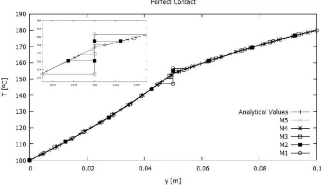
3.1.2 Results and Discussion

The results for the temperature distribution, with perfect contact and contact resistance interface, were obtained for several meshes using the developed code, to perform a comparison with the ones given by the analytical solution. For the temperature distribution at the line x = 50 mm, obtained with a perfect contact interface, illustrated in Fig. 6, it is noticeable that the temperature values obtained with the developed code, far from the interface, are coincident with the analytical ones, this even for the M1 which is the coarser mesh employed. Focusing on the interface, the values obtained with the analytical solution, at the same line, is 153.25ºC for the bottom slab and 153.38ºC for the top slab. Since it is modelled as perfect contact there should be no discontinuity on the temperature value at the interface, although, for the coarser meshes of the developed code results, a temperature discontinuity is predicted. This difference between the temperatures on each side of the interface gets smaller with the mesh refinements which means that the results are converging and by the M4 the discontinuity is practically inexistent and thermal continuity on the interface is almost achieved.

Fig. 6 – Analytical and numerical results for the temperature distribution of the Verification 1 case study: perfect contact

The convergence order values, Table 1, for the developed code show a good convergence of the results, when compared with the analytical ones. The order of convergence is close to second order,

18

which is expected, considering that the discretisation approaches employed (see Section 2.3) are second order as well.

Regarding the temperature distribution illustration in Fig. 7, considering that a perfect contact interface does not predict a temperature discontinuity between both regions, it shows, as expected, a continuous distribution at the interface.

Table 1 - Convergence order for perfect contact results of the Verification 1 case study

Numerical Values L∞ Error Convergence order

Mesh Edge Length [mm] S1 [ºC] S2 [ºC] S1 [ºC] S2 [ºC] S1 S2

M1 10 146.89 156.56 6.36 3.18 - -

M2 5 150.17 154.92 3.08 1.54 1.91 1.91

M3 2.5 151.76 154.12 1.49 0.74 1.91 1.91

M4 1.25 152.54 153.72 0.71 0.35 1.85 1.82

M5 0.625 152.93 153.52 0.31 0.15 1.72 1.62

Fig. 7 – Temperature [ºC] distribution for the perfect contact interface, calculated by the developed code with M5

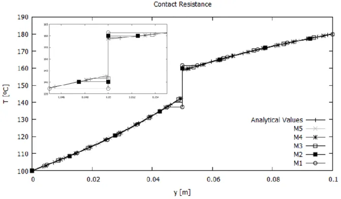
The results of the temperature distribution with the interface modelled with contact resistance, illustrated in Fig. 8, were obtained for several meshes on the line x = 50 mm across both slabs. Considering that, in this case, a contact resistance interface was employed, a temperature discontinuity

is expected to be obtained at the interface, which is shown by the analytical results where the values are 142.97ºC and 158.51ºC at the interface. Analysing the results on Fig. 8, as happened for the perfect contact case, the temperature values far from the interface are coincident with the analytical one. Although the values at the interface for the coarser meshes are considerably different from the analytical ones, the expected temperature discontinuity occurs at the interface. Setting the focus on the interface values, it is clear that the results obtained with the developed code converge to the analytical values with the mesh refinements. The results plotted on Table 2, show again a second order for the convergence, which is in accordance with the discretisation approaches employed for the governing equations terms, described in Section 2.3.

20

Fig. 9 – Temperature [ºC] distribution for the contact resistance interface, calculated by the developed code with M5

The temperature distribution, illustrated in Fig. 9, shows, as expected, a clearly defined temperature discontinuity between both regions.

The results obtained with both case studies presented in this sections, allowed to verify the developed code when diffusion is the only heat transfer process, since, in both cases, none of the domain parts is moving. The order of convergence was close to second order for both cases, as expected by the discretisation approaches employed to discretize the governing equation terms (see Section 2.3).

Table 2 - Convergence order for resistance contact results of the Verification 1 case study

Numerical Values L∞ Error Convergence order

Mesh Edge Length [mm] S1 [ºC] S2 [ºC] S1 [ºC] S2 [ºC] S1 S2

M1 10 137.20 161.40 5.77 2.88 - -

M2 5 140.15 159.92 2.82 1.41 1.94 1.94

M3 2.5 141.57 159.21 1.40 0.70 1.97 1.98

M4 1.25 142.27 158.86 0.70 0.35 1.99 1.98

3.2 Verification 2 – “Complex Layout”

A more complex problem is here developed to test the code for a more difficult and more similar model with the one being developed in this project. The temperature distribution obtained with the developed code are compared with the one given for the same model and available on the scientific literature, Nóbrega J. M. et al. (2004). This 2D layout is composed by a polymer sheet and a calibrator, as illustrated on Fig. 10. The polymer sheet is moving, at a constant and uniform velocity, while the calibrator is stationary. For this case, diffusion and advection transport mechanisms were considered, due to the fact that the polymer sheet is moving. Concerning the boundary conditions, the polymer sheet, has an inlet fixed temperature and, the calibrator, has a fixed temperature imposed on the cooling channels. A mesh convergence study was also performed to evaluate how the results behave with mesh refinement changes. For this study, six meshes, with different refinement levels, were used to obtain the temperature distribution in different locations with the developed code, the L2 error, defined as |𝑥| = √∑𝑛 |𝑥_𝑘|2

𝑘=1 , where 𝑥𝑘 is the value of the difference between the result obtained and the reference

one, was calculated and using number of cells of each mesh the convergence order was calculated, as described by S. Clain et al. (2013). Due to the fact that, for this case study, an analytical solution was not available, the L2 error was obtained using a reference value. This reference value was obtained by refining the mesh until no variations on the results was achieved and when subsequent mesh refinements obtained the same results, these were used as reference.

22

3.2.1 Computational Model

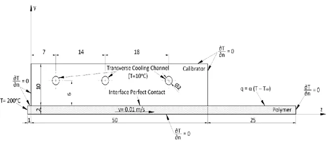
The geometry of this model, Fig. 10, is 2D and composed by two different regions, the polymer and the calibrator. The polymer region is located at the bottom, has a total length of 76 mm and a thickness of 2 mm. This region is in contact with the calibrator on the total length of the later, which is 50 mm. The calibrator region has a 10 mm thickness, is located on top of the polymer region and contains three transverse cooling channels. These transverse cooling channels have a 2 mm diameter and they are located at 7, 21 and 39 mm distance from the left edge of the calibrator. This is a slightly modified version of the case study proposed by Sheehy et al. (1994), where the inlet location on the polymer region is slightly displaced to the left, where the original is aligned with the calibrator left edge. When using the Finite Element Method to discretize the governing equations, this alignment creates an unrealistic scenario, where the temperature gradient in direction normal to the interface is null, a direct consequence of assuming that the temperature of the calibrator next to the polymer is equal to the melt inlet temperature, as explained by Nóbrega J. M. et al. (2004).

Regarding the physical and thermal properties employed in each region of this model, as described by Sheehy et al. (1994), for the calibrator region the thermal conductivity was defined as 𝑘_𝑐 = 23 W/mK, on the other hand, for the polymer region, the thermal conductivity was defined as 𝑘_𝑝 = 0.18 W/mK, the density as 𝜌_𝑝= 1400 kg/m3 and the heat capacity as 𝑐

𝑝 = 1000 J/kgK.

There are several boundaries that were used to model this verification, as illustrated on Fig. 10. For the polymer region a fixed inlet melt temperature of 200ºC was used on the left side, the bottom edges, the end of the polymer section and the small edge between the inlet and the calibrator were defined as insulated. The top edge, on the last polymer section that is not in contact with the calibrator, is defined as free convection. Regarding the boundaries used on the calibrator region the outer edges were defined as insulated and the cooling channels have a fixed temperature of 10ºC. To finish the modelling of this verification in terms of boundary conditions, the interface between the polymer and the calibrator region was modelled as perfect contact.

The mesh used to obtain the final results of this verification was constructed using Salome and the Netgen meshing algorithm. This is a mesh composed by triangular shape cells. Part of the M6 is illustrated on Fig. 11, this mesh has a total of 217914 cells and the minimum and maximum edge length is, respectively, 0.067 mm and 0.179 mm. Regarding the other meshes, used on the convergence study, the same procedure was used to obtain them (see Section 3.1.1). The number of cells for M1, M2, M3, M4 and M5 is, respectively, 298, 1016, 3380, 13520, 54698.

Fig. 11 – Verification 2 case study mesh M6

3.2.2 Results and Discussion

A convergence order study was conducted to evaluate the convergence of the results obtained with the six meshes described in the previous section. For this study the results were obtained on a line crossing both regions, polymer and calibrator, located at 𝑧 𝐿⁄ = 7 50⁄ , illustrated in Fig. 12. The L2 errors and convergence order are shown on Table 3. Analysing the convergence order values for all locations, a close to second order value is achieved, which is expected considering the discretisation approaches employed (see Section 2.3). Bottom line for all locations a good agreement between the results is obtained with the M6, making it trustable to be use to obtain the final results.

24

Table 3 – L2 errors and convergence order for the complex layout on the locations z/L = 7/50, 30/50 and 50/50

L2 Errors [ºC] Convergence Order z/L = 7/50 z/L = 30/50 z/L = 50/50 z/L = 7/50 z/L = 30/50 z/L = 50/50 Mesh_1 3217.55 2547.22 2840.61 - - - Mesh_2 951.20 751.68 940.39 1.76 1.76 1.59 Mesh_3 275.70 191.65 224.67 1.79 1.97 2.07 Mesh_4 82.18 55.21 74.01 1.75 1.80 1.60 Mesh_5 20.34 15.63 21.74 2.01 1.82 1.77 Mesh_6 5.13 4.36 5.91 1.99 1.84 1.88

Fig. 12 - Results for several meshes on the location 7/50 of the complex layout, benchmark from Nóbrega J. M. et al. (2004)

The Fig. 12 also contains the results obtained by Nóbrega J. M. et al. (2004) for the same location allowing to understand how the results obtained with the developed code evolve with the mesh refinement. Analysing the results obtained with the developed code and compare them with the reference ones, M1 do not show a good agreement with the benchmark results. At this location, with M1, the temperature values decrease linearly throughout the polymer region and the temperature value on the interface is significantly different from the benchmark value. Although the model starts to show better agreement with

the M3 showing already a non-linear temperature decrease in the polymer region and the temperature value on the interface is closer to the benchmark one. The results obtained with M4, M5 and M6 are coincident with the benchmark values, showing a good agreement regarding the temperature distribution throughout both regions.

The temperature distribution, obtained using the developed code, across both polymer and calibrator regions is illustrated on Fig. 13. Four different locations were used to compare and analyse the results, retrieved by the developed code. These locations follow the same relation 𝑧 𝐿⁄ and the locations used were 7/50, 30/50, 50/50, 75/50. The first location crosses the first cooling channel, the second one is approximately in the middle of the calibrator, the third is at the end of the calibrator region and, the last one, is at the end of the polymer region, this one only contain temperatures of the polymer section. The results were grouped in the Fig. 14 along with the reference results for the same locations.

Fig. 13 - Temperature distribution illustration for the Verification 2, with M6

Analysing the results of the Fig. 14, it shows that the results obtained with the developed code are in agreement with the benchmark ones, except for the location 75/50 which is not in total agreement, this might happen due to the fact that the mesh used in this study was a lot more refined than the one used on the benchmark study. For the locations 7/50, 30/50 and 50/50 the agreement is clear throughout all temperature values. Moreover, the numerical results predict a continuous temperature distribution at the interface between the polymer and the calibrator, as expected, since the interface was modelled as perfect contact.

26

Fig. 14 - Temperature distribution for the Complex Layout case study, with M6. Benchmark from Nóbrega J. M. et al. (2004)

The developed code results, as stated, obtained a very good agreement when compared with the benchmark ones. This allows to conclude that the developed code is able to handle more complex layouts, even with moderately mesh refinements.

4. POLYMER CALIBRATION CASE STUDY

The numerical code, verified in Chapter 3, is now going to be used to study the cooling and calibration stage of the polymer extrusion process. The objective is to evaluate the influence of the boundary conditions, geometrical and process parameters on the performance of the cooling system. For this, three different studies were conducted, where two of them have the same process parameters employed although the layout polymer/calibrator is different between them and, the third one, different geometrical and process parameters were applied on the model and its influence, on the final results, is analysed. The same studies were conducted by Nóbrega, J. M. et al. (2004) and were used here to validate the numerical code developed in this work. These studies allow to evaluate the developed code capabilities in different geometries and under different conditions.

The cross section for all the following studies is shown in Fig. 15, except on the studies where the geometrical parameters of the calibrators are changed. This cross section is composed by a polymer part, on the inside, with a 70 mm x 60 mm rectangular outer contour and a 3 mm thickness, the calibrator part is positioned around the polymer with a 130 mm x 120 mm rectangular outer contour. This part also contains four transverse cooling channels with 8 mm of diameter and located at 12 mm from each profile cross-section edge. This is a simple cross section, although it is ideal to perform the first studies with a recently developed code.

28

The Table 4 describes the general/reference conditions and properties used in the studies.

Table 4 - Conditions and Properties used on the studies, Nóbrega J. M. et al. (2004)

Conditions and Properties Used

k

kc 14.0 W/mK

ρp 1400 kg/m3

cp 1000 J/kgK

Linear extrusion velocity 2 m/min

Inlet temperature 180ºC

Room temperature 20ºC

Cooling fluid temperature 18ºC

Free convection heat transfer coefficient 5 W/m2K

Contact resistance heat transfer coefficient 500 W/m2K

The subscripts p and c stand for, respectively, polymer and calibrator. In terms of the conditions presented on the Table 4, the linear extrusion velocity is constant and applied only on the polymer region and the Inlet temperature is only applied on the profile inlet. The room temperature is a variable used when free convection at the outer walls is considered, on both polymer and calibrator regions, when this happens the free convection heat transfer coefficient is also used and both of these conditions are always constant. At the cooling channels walls a fixed and constant temperature of 18ºC is considered. The table last entry is the heat transfer coefficient considered when modelling the interface between the polymer and the calibrator regions.

The Table 5 presents the different conditions, used on the model, for the different studies conducted. Two different types of conditions are considered, the boundary used at the outer walls of the polymer and calibrator regions and the heat transfer coefficient considered at the interface between the two regions. For the outer walls, two different cases are considered, the first is to use convection, which is having a heat flux leaving or entering the system through the outer walls, and the second is to consider the entire system insulated, meaning that no energy is lost through the outer walls. Another condition that could be considered on the outer walls is the radiation, although this condition has no effect on the results, as shown by Nóbrega J. M. et al. (2004), and was not considered in this work. Regarding the heat transfer coefficient used at the interface, three different values are going to be used, the perfect contact, which considers that there is no contact resistance at the interface, and the contact resistance with different thermal resistance. The code notation presented in Table 5 refers to an easier way to identify

the different cases solved, c1 means that convection is used on the outer walls, c0 means no convection, h+ an increase of 50% on the heat transfer coefficient on the interface, h- a decrease of 50% on the heat transfer coefficient and pc stands for perfect contact.

Table 5 - Different conditions for outer surfaces and interface polymer/calibrator, Nóbrega J. M. et al. (2004)

Different Conditions Studied

Code Boundary for _{Outer Surfaces} Calibrator/Profile _{interface [W/m2K]}

c1 Convection 500

c0 Adiabatic 500

h+ Convection 750

h- Convection 250

pc Convection Perfect Contact

4.1 Three Calibrators Layout

This model is constructed using the previous shown cross section and it comprises using the polymer profile and three calibrators, with an annealing zone between each one of the calibrators, as illustrated in Fig. 16.

The developed code is going to be used to obtain the temperatures on the polymer profile cross section and the heat fluxes on the boundaries of the polymer and calibrators regions for the different cases on the Table 5.

The geometry of this model has four different parts, the polymer profile and three calibrators. The polymer profile has a total length of 850 mm and it cross section is the one described on Fig. 15, this part also has two annealing zones with 75 mm length when crossing from one calibrator to another. The three calibrators of the geometry keep the same cross section of the Fig. 15 and have a total length of 200 mm, they have a separation of 75 mm from each other and are in contact with the polymer profile on the inner walls across the total length of each of them.

30

Each part of the geometry can be divided into different zones, for the polymer profile it is divided into the zones OS1, OS2, OS3, OS4 and one zone for each calibrator that it crosses. This is done to allow different boundary treatment in each of the zones. In terms of boundaries used in the zones OS1, OS2, OS3 and OS4, these will have two different states which are being insulated and considering convection on them. The zones when crossing the calibrators are considered as contact resistance, with the different heat transfer coefficients that are on the Table 5, and perfect contact, being these zones an interface between the polymer region and the calibrator regions. The inner walls of the polymer profile are always modelled as insulated. Regarding the boundaries used on the calibrators, the outer walls consider two situations, convection and insulation, the inner walls in contact with the polymer profile are modelled as contact resistance and perfect contact depending on the case being solved (Table 5) and the cooling channels that can be seen on the cross section (Fig. 15) have a fixed temperature condition, these are used in each one of the calibrators.

The Fig. 17 illustrate the mesh used to obtain the final results of this case study. This mesh was constructed using the Salome software and the NetGen meshing algorithm. The parameters were defined on the algorithm, retrieving a mesh, M5, with 39 million cells, all of them of the Tetrahedra type, with a minimum and maximum edge length of, respectively, 0.054 and 3.099 mm. Regarding the number of cells of the meshes used on the convergence study, M1, M2, M3, M4 have, respectively, 9972, 75492, 550731, 4591662.

Fig. 17 – Three calibrator case study mesh

4.2 One Calibrator Layout

The second study performed using the developed code in presented in this section. In this case study the same cross section of the previous case is used, the layout, although, is composed with only one calibrator and the polymer profile, illustrated on Fig. 18. The developed code is going to be used to obtain the heat fluxes on the boundaries and temperatures at the end of the polymer profile cross section for the different studies shown on the Table 6.

32

The geometry of this model is constructed with two parts, the calibrator and the polymer profile, both have the cross section of the Fig. 15. The polymer profile has a total length of 700 mm and has three different zones, the OS1, OS2 and the interior that is in contact with the calibrator, the first two are not in contact with any specified region and have a length of 50 mm each, the third has the same length of the calibrator. The calibrator has a total length of 600 mm, being in contact with the profile on the inner surfaces. In terms of boundary conditions used in each zone, regarding the polymer profile the OS1 and OS2 zones use convection or insulation and the contact established with the calibrator is perfect contact and contact resistance, with different heat transfer coefficients. On the calibrator the outer surfaces use convection or insulation, the interior surfaces in contact with the polymer profile use perfect contact and contact resistance with different heat transfer coefficients and the cooling channels use a fixed temperature of 18ºC.

The mesh used in this study, illustrated in Fig. 19, was obtained using Salome and the Netgen algorithm, same as the previous case study. The same mesh refinement level obtained on the previous convergence study was using in this mesh, which retrieved a mesh with around 31 million cells of the Tetrahedra type, with a minimum and maximum edge length of, respectively, 0.0065 and 4.5898 mm.

4.3 Process and Geometrical Parameters

The previous case studies were used to evaluate the results behaviour when the boundary conditions on the outer surfaces and on the interface between the polymer and the calibrator were changed and also the number of calibrators, a geometrical parameter. This was also used to further assess the developed code, when tested with different boundary conditions, which performed qualitatively well on the several different cases solved.

The following case study uses, several more, process and geometrical parameters that can be changed in a real situation. The temperatures at the end of the cross section and the total heat removed from the polymer profile was obtained with the developed code. With this study, it is possible to identify how much the process parameters influence the final results, as well as the influence of the geometrical parameters. This also allows to choose the best parameters to apply on the cooling and calibration stage of the extrusion process.

To study the influence of the process and geometrical parameters, the one calibrator layout (see Section 4.2) was used with the conditions of the c1 case (see Table 5), except when a specific process parameter was changed. The parameters changed are shown on the Table 6. Regarding the process parameters, the cooling fluid that is present on the cooling channels of the calibrator is going to be used with two different temperature values, 12 and 24ºC, as well as the profile velocity is going to be used with the values 1 m/min and 3 m/min. Considering that these values, on the c1 case, are 18ºC and 2 m/min for cooling fluid temperature and profile velocity, respectively, a change of 50% above and below the reference values is applied.

The geometrical parameters are important in terms of the calibrator performance, some more than others, which this study is able to obtain enough data to identify how the parameters influence the performance. The first geometrical parameter considered was the number of calibrators used, which is similar to the three calibrator layout, where the total length of the one calibrator is divided by three calibrators and annealing zones are created between them. The second geometrical parameter is the position of the cooling channels on the calibrator, for the reference case they are at the middle of each side of the profile and here their location is changed to two different situation. The first moves, the four cooling channels, close to the corners of the profile, on the other hand, the second places two cooling channels next to each other, also meaning that the number of cooling channels is increased to eight. The last two geometrical parameters considered are the distance between the centre of the cooling channel and the profile surface, again with a value of 50% above and below the reference value. The other and

34

last parameter considered is the cooling channels diameter, changing its value to 50% above and below the reference case diameter.

Table 6 - Process and geometrical parameters used

Code Parameter Description/Value

Process Parameters

tw +

Cooling Fluid Temperature 12ºC

tw - 24ºC

vp +

Profile Velocity 1 m/min

vp - 3 m/min

Geometrical Parameters

nc Number of Calibrators

Divide the total cooling length into three individual calibrators

la

Cooling Channels Layout

Four cooling channels close to the profile's

corners

lb Two cooling channels _{next to each other}

cd + Distance between cooling

channels and profile surface

8 mm

cd - 16 mm

dw +

Cooling channels diameter 4 mm

dw - 12 mm

4.4 Mesh Sensitivity Study

A convergence order study was first performed to evaluate the convergence of the results when the mesh refinement degree is changed, it is expected to obtain results with a higher error with coarser meshes and this study also allows to identify what level of refinement should be used, to obtain trust worthy results for the model being studied. The procedure to obtain the convergence order is the one described by S. Clain et al. (2013) where the equation used was 𝑜𝑟𝑑 = 2 ln (𝑒𝑟𝑟𝑜𝑟(𝑀1)

𝑒𝑟𝑟𝑜𝑟(𝑀2)) ln ( 𝑀2 𝑀1)

⁄ where the

factor 2 was changed to 3 since this is a 3D mesh. The error was calculated as the difference between the value of the total heat flux obtained with the developed code and the value obtained using the Richardson extrapolation method.

For every mesh the heat fluxes through the boundaries were calculated, using the developed code. Then the total heat flux removed from the system was used to calculate the order of convergence. The Table 7 shows the results and errors for each mesh, the mesh information and the convergence order using the case c0.

Table 7 - Results and convergence order for the three calibrator layout, case c0 c0 N.º Cells Total Heat Flux [W] Error [W] Convergence Order M1 9972 -2128.03 1245.47 -- M2 75492 -2180.93 1192.57 0.06 M3 550731 -2237.15 1136.35 0.07 M4 4591662 -2901.48 472.02 1.24 M5 39118817 -3336.37 37.13 3.56 Richardson Extrapolation -3373.50

Regarding the results it is clear that for the coarser meshes, that is M1, M2 and M3, the total heat flux result is far from the expected and the convergence for those mesh refinements is small, with values of 0.06 and 0.07. This means that, for this model, it is required at least a refinement level like the M4 one, to obtain good results. Analysing the results for M4, here a large difference from the M3 is obtained, which ends up with a higher and more desirable convergence order, although since the difference was quite considerable another mesh refinement was required. Regarding the last mesh, M5, the error is smaller when compared to the M4 one, as expected, obtaining a larger convergence order towards the expected value, which allows to consider that the M5 refinement level is adequate for this model.

4.5 Influence of the Boundary Conditions and Number of Calibrators

The results for the case studies of the Table 6 for the three calibrator layout, comparing the heat fluxes at the boundaries and the temperatures on the profile cross section, are summarized on the Table 8 and Table 9. To obtain these results the wallHeatFlux and the patchAverage utilities of OF were used, where the first calculates the heat fluxes through the boundaries and, the later, provides the average value of a certain field on a specific boundary. This allows to understand how much energy each calibrator removes from the polymer profile and also what quantity of that energy is absorbed by the cooling channels. It is also possible to quantify how much energy is lost through the outer walls, as well as how