Influences of external factors in automotive sales forecasting : a portuguese case study

i

Influences of External Factors in Automotive

Sales Forecasting

Felipe Orestes Cuan Suárez Blanco

A Portuguese Case Study

Dissertation presented as partial requirement for obtaining

the Master’s degree Information Management

I

NOVA Information Management School

Instituto Superior de Estatística e Gestão de Informação

Universidade Nova de Lisboa

INFLUENCES OF EXTERNAL FACTORS IN AUTOMOTIVE

SALES FORECASTING

by

Felipe Orestes Cuan Suárez Blanco

Dissertation presented as partial requirement for obtaining the Master’s degree in Information Management, with a specialization in Business Intelligence.

Advisor: Jorge Morais Mendes, PhD

II

“It is often said there are two types of forecasts ... lucky or wrong!”

III

ACKNOWLEDGEMENTS

Firstly, I would like to express my sincere gratitude to my advisor, Professor Jorge Mendes, for his continuous support during my research, for his patience, motivation and knowledge. His guidance helped me all the time while doing research and writing of this dissertation.

Besides my advisor, I would like as well to thank Eng. Ricardo de Almeida for inspiring me to write about this subject and also for sharing his comprehensive knowledge and wisdom. I hope to, one day, reach such level of expertise.

My sincere thanks also go to my family, my dearest Camila Steiner, José Mourinho, Fátima Bernardes, Rita Meneses, Francisco Lourenço and João Santos who, without their precious patience, knowledge and support, this dissertation would not have seen the light of day.

IV

ABSTRACT

This study aims to contribute to a better understanding of the Portuguese automotive market, its behaviour and, additionally, attempt to create better sales prediction models, using linear regression models with ARIMA errors.

Through time series analysis, it will be studied how external factors such as socio-economic variables, consumer behaviour as well as market specific factors (e.g. gas prices, car rental services) affects the development of the automotive market. Furthermore, it will be tested if methodologies such as hierarchical forecasting on a bottom-up approach will bring better results compared to forecasting the market as a whole.

This understanding and forecasting techniques, if proven successful, can bring higher competitive advantage to companies in this sector, through more accurate planning and strategic management.

KEYWORDS

V

INDEX

1. Introduction ... 1

2. Literature review ... 2

3. Methods and theoretical framework ... 4

3.1.Data Gathering ... 5

3.1.1.Vehicle Sales ... 5

3.1.2.Addicional Data and External Factors ... 5

3.1.3.Data Preparation ... 6

3.2.Analysis ... 7

3.2.1.Time Series Analysis ... 7

3.2.2.Choosing and Fitting Models ... 7

3.2.3.Relationships between the vehicle registries and external factors ... 9

3.2.4.Hierarchical forecasting ... 10

4. Portuguese Vehicle Market ... 11

4.1.Characterization ... 11

4.1.1.Passenger Market ... 12

4.1.2.Commercial Market ... 13

4.2.Modelling and Forecasting - Total Sales ... 14

4.2.1.ARIMA Estimation and Order Selection ... 15

4.3.Forecasting Total Sales with outliers ... 17

4.4.Forecasting Total Sales with External Factors ... 20

4.4.1.Factors with some evidence of Correlation ... 21

4.4.2.Spurious Correlations ... 21

4.5.Modelling and Forecasting using Regression with Arima Errors... 22

5. Hierarchical Forecasting - Vehicle Market as a Sum of Parts ... 24

5.1.Forecasting Total Sales in a one Level Hierarchy: Car Rental + Free Market ... 24

5.1.1.Forecasting Car Rental ... 24

5.1.2.Forecasting Free Market ... 27

5.1.3.Results ... 29

5.2.Forecasting Total Sales in a One Level Hierarchy: Passenger + Commercial ... 30

5.2.1.Forecasting Passenger Market ... 30

5.2.2.Forecasting Commercial Market ... 32

5.2.3.Results ... 34

VI

5.3.1.Forecasting Passenger Car Rental ... 35

5.3.2.Forecasting Passenger Free Market ... 37

5.3.3.Total Market Results ... 39

6. Conclusions ... 40

6.1.Summary of Findings ... 40

6.2.Conclusion ... 40

6.3.Future Work... 41

7. Addendum ... 42

7.1.Model Comparison (using unchanged parameters) ... 43

7.2.Model Parameter Re-estimation ... 43

8. Bibliography ... 45

VII

LIST OF FIGURES

Figure 1 – Time series cross-validation. ... 8

Figure 2 - Multi-level hierarchy ... 10

Figure 3 – Historical Time Series of total vehicle sales ... 11

Figure 4 – Seasonality ... 11

Figure 5 – Relative percentage of passenger vehicle sales, per brand (red is higher) ... 12

Figure 6 – Relative percentage of passenger vehicle sales, per segment ... 12

Figure 7 – Relative percentage of passenger vehicle sales, per displacement ... 12

Figure 8 – Relative percentage of passenger vehicle sales, per fuel type ... 12

Figure 9 – Relative percentage of commercial vehicle sales, per brand ... 13

Figure 10 – Relative percentage of commercial vehicle sales, per segment ... 13

Figure 11 – Relative percentage of commercial vehicle sales, per displacement ... 13

Figure 12 – Relative percentage of commercial vehicle sales, per fuel type ... 13

Figure 13 – Original series (left) vs Box-Cox Transformation (right) ... 14

Figure 14 – Time series first order differentiation ... 14

Figure 15 – Auto-Correlation Functions for total sales ... 15

Figure 16 – Outlier detection - Total Sales ... 17

Figure 17 – Subset Model diagrams – Adjusted R2 and Mallow’s Cp for Total Sales ... 19

Figure 18 – Cross Correlation table – Total Sales ... 21

Figure 19 – Subset Model diagrams ... 22

Figure 20 – One level hierarchical forecasting: Car Rental + Free Market ... 24

Figure 21 – Car Rental time series and seasonal plot ... 24

Figure 22 – Outlier detection – Car Rental ... 25

Figure 23 – Free Market time series ... 27

Figure 24 – Outlier detection – Free Market ... 27

Figure 25 – One level hierarchical forecasting: Passenger + Commercial vehicles ... 30

Figure 26 – Passenger Market time series ... 30

Figure 27 – Outlier detection – Passenger Market ... 30

Figure 28 – Commercial Market time series ... 32

Figure 29 – Outlier detection – Commercial Market ... 32

Figure 30 – Two levels hierarchical forecasting ... 35

Figure 31 – Passenger Car Rental time series ... 35

Figure 32 – Outlier detection – Passenger Car Rental ... 35

Figure 33 – Passenger Free Market time series ... 37

Figure 34 – Outlier detection – Passenger Free Market ... 37

Figure 35 – Error measure (MAPE) of best models ... 40

Figure 36 – Historical Time Series of total vehicle sales ... 42

Figure 37 – Historical Time Series of total Car Rental ... 42

Figure 38 – Error (MAPE) model comparison using the same parameters ... 43

Figure 39 – Error (MAPE) for total vehicle sales ... 43

VIII

LIST OF TABLES

Table 1 – External Factors ... 6

Table 2 – ARIMA models overview – Total Sales ... 16

Table 3 – Outliers – Total Sales ... 18

Table 4 – Regression coefficients – Total Sales with outliers ... 18

Table 5 – Final Regression coefficients – Total Sales with outliers ... 19

Table 6 – ARIMA models overview – Total Sales with outliers ... 20

Table 7 –Regression coefficients – Total Sales with outliers and external factors ... 22

Table 8 –Final Regression coefficients – Total Sales with outliers and external factors ... 23

Table 9 – ARIMA models overview – Total Sales with outliers and external factors ... 23

Table 10 – Outliers – Car Rental ... 25

Table 11 – Regression model - Car Rental with outliers ... 25

Table 12 – Cross Correlation table – Car Rental ... 26

Table 13 – Regression model - Car Rental with outliers and external factors ... 26

Table 14 – ARIMA models overview – Car Rental ... 27

Table 15 – Outliers – Free Market... 27

Table 16 – Regression model – Free Market with outliers ... 28

Table 17 – Cross Correlation table – Free Market ... 28

Table 18 – Regression model – Free Market with outliers and external factors ... 29

Table 19 – ARIMA models overview – Free Market ... 29

Table 20 – Forecast aggregation: Car Rental + Free Market ... 29

Table 21 – Outliers – Passenger Market ... 31

Table 22 – Regression model – Passenger Market with outliers ... 31

Table 23 – Cross Correlation table – Passenger Market ... 31

Table 24 – Regression model – Passenger Market with outliers and external factors ... 32

Table 25 – ARIMA models overview – Passenger Market ... 32

Table 26 – Outliers – Commercial Market ... 33

Table 27 – Regression model – Commercial Market with outliers ... 33

Table 28 – ARIMA models overview – Commercial Market ... 34

Table 29 – Forecast aggregation: Passenger + Commercial Market ... 34

Table 30 – Outliers – Passenger Car Rental ... 36

Table 31 – Regression model – Passenger Car Rental with outliers ... 36

Table 32 – Cross Correlation table – Passenger Car Rental ... 36

Table 33 – Regression model – Passenger Car Rental with outliers and external factors ... 36

Table 34 – ARIMA models overview – Passenger Car Rental ... 37

Table 35 – Outliers – Passenger Free Market ... 37

Table 36 – Regression model – Passenger Free Market with outliers ... 38

Table 37 – Cross Correlation table – Passenger Free Market ... 38

Table 38 – Regression model – Passenger Free Market with outliers and external factors ... 38

Table 39 – ARIMA models overview – Passenger Free Market... 39

1

1. INTRODUCTION

Success in market oriented companies depends not only on carrying effective management on daily basis but also on the ability to understand the intricate factors that shape the fabrics of the economy and, even better, to foresee and correctly assess changes in the future.

Due to socio-economic fluctuations and changing trends, this reality is present in many sectors of activity and is especially true in the automotive industry. The creation and development of the automotive vehicle has created one of the biggest changes in mankind history, allowing much faster exchange of goods and people, rocketing civilization into the modern age. However, as society develops further and further, influences such as globalization, car overproduction and the demand for more customized products (Holweg, 2008) leads to more competition among companies.

In Portugal, the automotive industry generated 18 billion euros in 2013 (ACAP, 2016a), through manufacturing, sales and exports which represents a total of 15% of the GDP. In 2016, auto loan reached 860 million euros just in the first five months of the year (Godinho, 2016).

Taking into consideration the Portuguese automotive market, which is comprised by 55 brands (ACAP, 2016b), the ability for these competing companies to generate reliable forecasts is of the utmost importance, which cannot be left only to intuitive guesses on market development. Nowadays, where advancements in data collection allow quality information to be much more accessible (AutoInforma, 2016), analysis and mathematical modelling of such data can create means to generate more accurate, and consequently, more reliable forecasts than ever before.

Having this in mind, the objective of this study is to allow further comprehension on what influences the development of the automotive market, which are the major factors in a macroeconomic scale and if there are other variables, such as social features or market specific characteristics that allows to correctly access and, if possible, predict short term future.

This type of short term forecasting, as of one or two months ahead, is especially important to companies/brands that rely on market share to fulfil their goals as this allows to plan ahead their operations, logistics and marketing schedules while having in account effects such as seasonality and vehicle lifecycles. Up to 95% of total yearly sales belong to companies/brands that are massified for the consumer. These companies tend to relate their objectives to market share presence and thus work intimately with the method explained before. The other 5% belong to luxury brands that target specially the aficionado and set their objectives by the total yearly sales, independent of time.

2

2. LITERATURE REVIEW

Time series analysis applied to sales forecast was first introduced by Lewandowsky (1974), concerning particularly the German automotive industry. This author, along the studies of Berkovec (1985), Dudenhöffer and Borscheid (2004) over automotive market modelling and sales forecasting established the foundations of time series analysis in this sector.

To accurately forecast, it is important to assess the data and determine if there are any consistent patterns, significant trends or seasonality and it is also important to find out if there are any outliers that can to be explained. While this analysis is done univariately, external factors - secondary time series parallel in time with the main time series – may have influence on the trend development, which adds another layer of complexity.

Concerning this last point, Brühl, Hülsmann, Friedrich and Reith (2009) analysed external factors of different natures, such as:

- Variables of global (national) economy - Specific variables of the automotive market - Variables of the consumer behaviour

Later on, this study was reviewed by Hülsmann, Borsheid, Friedrich and Reith (2012) enhancing the previous methodology.

In the Portuguese case, similar factors were analysed by Monteiro (2009) and Martins (2012). Monteiro concluded that unemployment and family income were factors that correlated with the market development while other factors such as tax load, end-of-life incentives or gas prices were not relevant. On the other hand, Martins concluded that both tax load and car-scrap bonus where relevant, opposing to unemployment rate which had little correlation with the market.

Faced with the disparity between these two studies and the lack of other literature regarding the influence of such factors in the Portuguese market, it would be interesting to determine which factors are indeed (if any) influencing the automotive market.

Also, to be noted is the influence of car rental services in the market development. These vehicles represent a significant portion of yearly sales – around 20% of the total market (ARAC, 2015), have a

3 very stable seasonality and normally are subject to contracts of fixed volume of sales. At the moment, there are no studies available regarding this subject in Portugal.

Other matter with relevant interest is that in a sector regulated by the competition law, transparent and detailed data of each company/brand is available (AutoInforma, 2016). Such data includes daily and monthly vehicle sales by segment, category and model. Having such structured information, one can question if the analysis and modelling of such components will bring better results compared to analysing the car market as a whole.

Having such broad perspective is important for companies in this sector as it allows them to plan their stocks, both strategically and tactically for their near future and, at the same time, “keep an eye” on their competitors.

One way to analyse this information is using grouped/ hierarchical forecasting, where the various components (e.g. car model, segment, category time series) can influence the modelling at higher levels (e.g. vehicle market) (Hyndman, Ahmed, Athanasopoulos and Shang, 2010).

Classical approaches involve top-down or bottom-up methodologies, or a combination of both. The top-down method forecasts the aggregated time series and then disaggregates it based on historical proportions (Gross and Sohl, 1990). The bottom-up method involves forecasting each disaggregated series at the lowest levels and uses simple aggregation operations to obtain forecasts at higher levels.

Having the broad perspective of the different aspects of the different aspects of the literature, this dissertation will focus on the following objectives:

O1 – Is it possible to create more accurate predictions recurring to hierarchical forecasting

compared with forecasting the market sales as a whole? If so, which type of segregation does bring better results: Car Rental or Vehicle Category?

O2 – Which external factors influence the most when correlating with the different market

4

3. METHODS AND THEORETICAL FRAMEWORK

To follow the proposed objectives and further elaborate on this research, the subsequent schematic diagram describes, briefly, the major stages and the process workflow:

Vehicle Sales Data Other Sources

Data Preparation

Time Series

Analysis Trends, Seasonality

Outlier Detection Determining Appropriate External Factors Cross Correlation function Fitting multiple linear regression model Box-Jenkins Methodology ARIMA Model MLR Models with ARIMA errors Model Evaluation and Validation Data gathering Data Preparation Analysis Modelling Validation

5

3.1. D

G

3.1.1. Vehicle Sales

The main data series is comprised by new vehicle registrations in Portuguese territory. This information is gathered and managed by the Portuguese Automotive Trade Association (ACAP). For this research was considered only light vehicles (i.e. gross weight less than 3500Kg and up to 9 seated places) in a time frame comprised between January 2006 to July 2016, with monthly and daily periodicity.

This data is divided by category, vehicle segment and brand. Vehicle category is defined by its purpose and usage, which can be for transporting passengers - Passenger Vehicle - or goods - Commercial Vehicle. Vehicle Segment adds another subdivision on passenger and commercial vehicles. It characterizes each vehicle according to its distance between wheel axis, engine power, price and bodywork.

3.1.2. Addicional Data and External Factors

To expand the complexity and enrich the mathematical models, additional data was gathered such as socio-economical indexes/indicators and specific automotive market data namely car rental statistics and oil prices.

Data regarding rental vehicles was gathered from the Portuguese Rent-a-Car Association (ARAC) which represents about 80% of all rental businesses. The available data is comprised by the number monthly vehicles delivered to rental companies, from January 2006 to July 2016, by brand.

Considering social-economic factors, this research will have in account factors previously used in studies such as Brühl et al (2009), Monteiro (2009), and Martins (2012). Additionally, other factors that were potentially interesting and relevant for this research were also considered.

A summary of the factors gathered are detailed in the table below:

Factor Description Type

R1 Unemployment rate of active population between 15 and 74 years old (%) Social R2 Private Consumption Indicator Economic R3 Economic Climate Indicator Economic R4 Expectations of unemployment evolution over the next 12 months Social R5 Expectations on economic climate over the next 12 months Economic R6 Consumer price index Economic

6

Factor Description Type

R7 Crude Oil price - Brent (EUR) Specific R8 Nights spent at tourist accommodation establishments - Residents Social R9 Nights spent at tourist accommodation establishments - Non-Residents Social R10 Appreciation on economic climate of the last 12 months Economic R11 Economic Activity Indicator (%) Economic R12 Employment Index on Industry Sector Social R13 Employment Index on Commerce Sector Social R14 Employment Index on Service Sector Social R15 Savings Opportunity Economic R16 Expectations of equipment good acquisition in the next 12 months Economic R17 Expectations on sales prices over the next 3 months Economic R18 Number of weekday holidays per month Calendar R19 Number of workdays per month Calendar R20 Expectations on demand on services over the next 3 months Economic R21 Expectations on demand in commerce over the next 3 months Economic R22 Salary Index on Industry Sector Economic R23 Salary Index on Commerce Sector Economic R24 Salary Index on Service Sector Economic

Table 1 – External Factors

3.1.3. Data Preparation

Even though all data is extracted from official and trustworthy sources, some data cannot be applied directly to the analysis as it needs validation and preparation. This task consists in verifying missing values and data discrepancies that may occur in the timeline.

There were no major issues aside from one or other missing value. To these specific cases it was applied values an interpolation function according to Stineman (Stineman, 1980).

Further transformations were required to adequate the data to their specific methodologies, such as taking in consideration for normalization, stationarity, heteroskedasticity and pre-whitening. These will be detailed in subsequent sections.

7

3.2.

A

3.2.1. Time Series Analysis

An exploratory allows determining main characteristics of time series such as:

- Trends – measurements that, on average, tend to increase or decrease over time.

- Seasonality - regular repeating patterns of highs and lows related to calendar time such as seasons, quarters, months, and days of the week.

3.2.2. Choosing and Fitting Models

This research will focus in modelling using Box-Jenkins Methodology and Linear Regression with ARIMA errors. These methodologies were chosen due to their popularity in the industry and proven efficacy in forecasting.

3.2.2.1. Box-Jenkins Methodology

As proposed by George Box and Gwilym Jenkins (1970), this methodology involves identifying an appropriate an autoregressive integrated moving average (ARIMA) process that fits into the data, and then using the computed fittedmodel for forecasting.

The original Box-Jenkins modelling process involves an iterative three-stage process of model: selection, parameter estimation and model checking. Recent developments of this process, as in Makridakis, Wheelwright and Hyndman (1998) and add a preliminary stage of data preparation and a final stage of model application, as in forecasting and validation.

1. Data preparation involves cleaning and transformation of data, as mentioned in the previous section. Transformation of the data helps to stabilize parameters such as mean and variance in a time series and guarantee they do not change over time. Since stationarity is an assumption underlying ARIMA models, unit root tests allows checking this characteristic. Examples of unit root test used in this research are Augmented Dickey–Fuller test or Kwiatkowski–Phillips–Schmidt–Shin (KPSS) test.

If a time series is non-stationary, transformations such as Box-Cox transformation and Differentiation are standard procedure to overcome such impediments.

2. Model selection in the Box-Jenkins methodology uses various tools such as analysing Auto-Correlation Function and Partial Auto-Auto-Correlation Function graphs on the transformed time series to try to identify potential ARIMA processes which might provide a good fit to the data.

8 3. Parameter estimation implies finding values for the model coefficients which provide the best fit to the data. To help in this process, there are measures that allow perceiving how well the model is fit. Examples of these are Akaike’s Information Criterion and Bayesian Information Criterion.

4. Model Checking involves testing the assumptions of the model to identify any areas where the model is inadequate. This can be done by analysing the residuals of the model as it is expected to have the appearance of white noise. Again, unit root tests and ACF graphs allow checking these traits.

If the model is found to be inadequate, it is necessary to go back to Step 2 and try to identify a better model.

5. Forecasting. Once the model has been selected, estimated and validated, it is then appropriate to use for forecasting. To measure forecast accuracy, last periods of the data should be left out of the modelling process to be used as testing data. In this study, accuracy of the model was done through cross-validation. This technique was also used by Hyndman (2014) and uses different training sets, each one containing one more observation than the previous one as shown in Figure 1 (The blue points are training sets, the red points are test sets and the grey points are ignored). The forecast accuracy measure is calculated on each test set and the results are averaged across all test set, adjusted to their different sizes. In this research, it was considered only a single forecast horizon, h, (next month) as it is the most crucial value to forecast. The accuracy measurement used was the mean absolute percentage error (MAPE).

Figure 1 – Time series cross-validation.

9

3.2.2.2. Linear Regression models with ARIMA errors

To take in account other relevant information such as calendar effects or external factors, regression models can be applied in these situations. When using regression models with time series, it is common for the residuals to have a time series structure.

This procedure follows the subsequent steps:

1. Use ordinary least squares regression to estimate the model yt=β0+β1R1t +β2Rkt+ϵt

where yt is a linear function of the k predictor variables (R1t,…, Rkt), and ϵt the residual series.

2. Examine the ARIMA structure (if any) of the sample residuals from the model in step 1. 3. If the residuals do have an ARIMA structure, use maximum likelihood to simultaneously

estimate the regression model using ARIMA estimation for the residuals.

4. Examine the ARIMA structure (if any) of the sample residuals from the model in step 3. If white noise is present, then the model is complete. If not, continue to adjust the ARIMA model for the errors until the residuals are white noise.

An important consideration in estimating a regression with ARMA errors is that all variables in the model must first be stationary. A regression with ARIMA errors is the same as a regression model in differences with ARMA errors.

In this research, having so many factors/variables to dissect may cause an issue of overfitting the regression model. Thus, to determine and choose the best and most useful predictors it followed the best subset regression approach, where it is computed all possible models and displayed a smaller subset of variables (predictors) along with their adjusted R-squared and Mallows' Cp values. The idea

is to understand which model presents the highest R2 along with the lowest Mallows’ Cp.

3.2.3. Relationships between the vehicle registries and external factors

To feed the correct variables/factors to the regression model it is necessary to assess which factors are indeed relevant for the regression model. One way to establish this relationship is to analyse the cross correlation function (CCF) between the main series (e.g. vehicle registries) and each of the exogenous factors as it identify which lags might be useful as predictors.

One major concern in the usage of CCF is that is affected by common trends that the two time series may have over time. A strategy to work around this difficulty is to use a pre-whitening procedure. This operation processes a time series to make it behave statistically as white noise thus reducing the presence of systematic information not relevant to prediction.

10

3.2.4. Hierarchical forecasting

As part of the proposed objectives for this study, it will be necessary to compare the accuracy of forecasts of the vehicle market as a whole, and the hierarchical methodology. The best model to apply will depend on the exploratory analysis and the relationships between main time series and the different external factors.

As for the hierarchical forecasting methodology, a multi-level hierarchy such as shown in figure 2 should be applied to the main time series, where level 0 is the complete aggregation series (i.e. total vehicle sales), level 1, the first level of disaggregation (i.e. Category: Passenger, Commercial, …) and level 2, the desegregation by brands in each of the correspondent categories.

Figure 2 - Multi-level hierarchy

This study follows the theory of optimal combination forecast in hierarchical time series developed by Athanasopoulos et al (2007) and Hyndman et al (2010) which share similarities to approaches from Solomon and Weale (1991, 1993, 1996).

11

4. PORTUGUESE VEHICLE MARKET

4.1. C

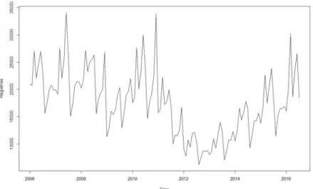
Figure 3 – Historical Time Series of total vehicle sales

The data gathered for this study revealed a very interesting period on automotive sales history as it can be observed in the figure above, between 2006 and 2009 there is a slight downward trend with occasional peaks before further reduction of sales. After 2011 and until 2013 the number of sales has plundered to numbers almost half of the previous years. Only after 2013 it is possible to see some recovery and a significant upward trend in the latter years.

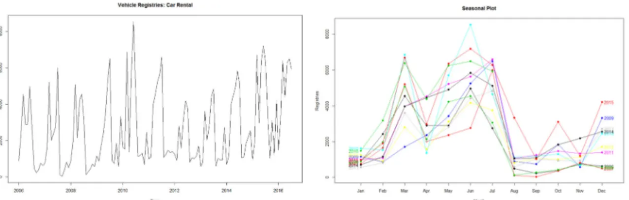
12 Regarding seasonality, the series shows a pronounced seasonal behavior. Each quarter has upward trends, with different levels, being the second quarter the one with highest slope and the third with the lowest. This behavior is intimately related with the way sales objectives/goals of the major brands are specified.

Another way to analyze data is though heat maps, using different vehicle characteristics to extract further knowledge. For this analysis it was chosen to segregate by type, brand, segment, displacement and fuel type.

4.1.1. Passenger Market

Figure 5 – Relative percentage of passenger vehicle sales, per brand (red is higher)

Comparing different passenger brands, it is interesting to see that before 2010 most of them had similar sales seasonality, reaching yearly highs around the middle of the year. However, after major sales drop during 2011-13 some brands haven’t recovered fully, with their sales dropping significantly. In recent years there has been some stabilization by the major players as the sales keep trending upward.

Figure 6 – Relative percentage of passenger vehicle sales, per segment

(A – Económico; B – Inferior; C - Médio-Inferior; D - Médio-Superior; E – Superior; F –Luxo; G – SUV; H – Monovolume)

Figure 7 – Relative percentage of passenger vehicle sales, per displacement

13 Comparing segment and displacement in the latter years, there is a tendency to choose vehicles with smaller displacement and lower segments. It should also be noted that there is an increasing preference of SUV’s (Segment G) and electrical/hybrid vehicles are starting accelerate in sales, even though their market share is still very small.

4.1.2. Commercial Market

Figure 9 – Relative percentage of commercial vehicle sales, per brand

Figure 10 – Relative percentage of commercial vehicle sales, per segment

(C -Chassis-Cabina; DTS - Derivado Tecto Sobreelevado; DV - Derivado Van; FM - Furgão de Mercadorias; FP - Furgão Passageiros; P4x2 - Pick-Up 4x2; P4x4 - Pick-Up 4x4)

Figure 11 – Relative percentage of commercial vehicle sales, per displacement

Figure 12 – Relative percentage of commercial vehicle sales, per fuel type

Observing commercial market, similar commentary as the passenger market can be concluded. In this case sales have diminished significantly after 2012 and smaller displacement engines are the preferred choice for newer vehicles. Also to be noted the downward trend for gasoline fuel source and an upward trend on bi-fuel and electrical, even though diesel is still prevailing as the main fuel source.

After this preliminary analysis and acquaintance of the market and the data, it is possible to start modelling.

14

4.2. M

F

-

T

S

For the purpose of modelling the time series it will be analysed the time series of vehicle sales as a whole as first approximation. It is necessary to contemplate transformations to accommodate the initial conditions for ARIMA models. Such conditions/hypothesis consists in checking stationarity and heteroscedacity.

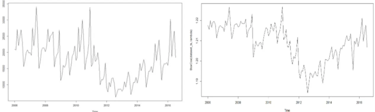
Following Guerrero (1993) methodology to test hetersocedacity, the time series will need a Box-Cox Transformation.

Figure 13 – Original series (left) vs Box-Cox Transformation (right)

To test for stationarity, it was used both Augmented Dickey-Fuller Test and KPSS Test for double validation.

Null hypothesis p-value

ADF Test Series in non-stacionary 0,8432

KPSS Test Series is stacionary 0,0100

Both tests confirm non-stacionarity and the need (and latter analysis the suficiency) for a first order differenciation.

Figure 14 – Time series first order differentiation

Though these transformations, it is possible to evidence a few outliers, which will be considered later on in the modelling process.

15 Onward and on other modelling applications, these transformations were applied whenever it was deemed necessary.

4.2.1. ARIMA Estimation and Order Selection

To proceed with order estimation, auto-correlation graphs were created for the time series.

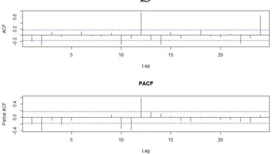
Figure 15 – Auto-Correlation Functions for total sales

The analysis of the auto-correlation functions shows evidence of high correlation of the second order on both ACF and PACF which in turn incline to a probable ARIMA model with (2,1,2) order as first approximation.

To determine the best model while having in account the preliminary ARIMA orders obtained through the auto-correlation graphs, it was calculated various models with permutations of the parameter orders based on the initial estimation. The process consisted on calculating models with parameters as permutations of orders in the neighborhood of the initial estimation.

The choice of the best model was done by choosing the top 10 models that minimize the Akaike Information Criteria (AIC) with general consensus of the other information criteria values (AICc and BIC) while also minimizing a 4-fold cross-validation error, having in account the values of unit root test for the residuals on different lags.

16

Table 2 – ARIMA models overview – Total Sales

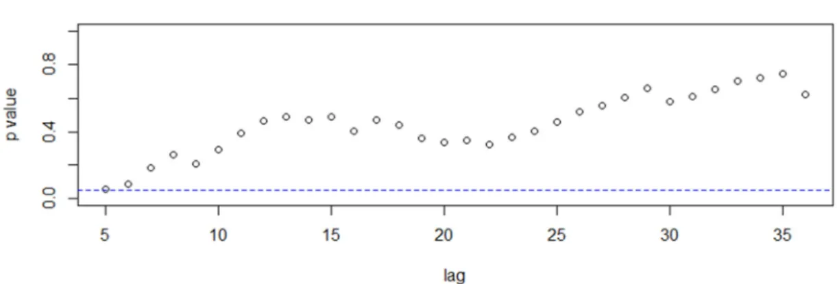
After choosing the best adequate model though this process, extensive analysis was done to ensure the validity and correctness of the model. This includes (1) the predicted values, (2) the values of the residuals, (3) histogram of the residuals, (4, 5) ACF and PACF of the residuals, (6) Q-Q Plot and finally (7) unit root test – Ljung-Box statistics – over the residuals. In this latter test is important to remind the null hipothesis states that the data is independently distributed, i.e. there is no serial correlation in the observation.

(1) (2) ₍₃₎

17 As all the validation tests have passed, the ARIMA (0,1,1)(1,0,2) model is considered viable as a forecasting model.

4.3. F

T

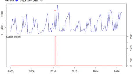
S

As it was mentioned before, there are outliers present on the window timeframe. Some are easily perceived, others are clearer after posterior transformations. To evidence the outliers in existence it was applied automatic outliers detection methodologies described by Cryer, J., Chan, K. (2012). Residuals are identified by fitting a loess curve for non-seasonal data and via a periodic STL decomposition for seasonal data. Residuals are labelled as outliers if they lie outside a specified quantile range of the residuals.

Figure 16 – Outlier detection - Total Sales

(7)

18 From the results of the outlier detection it is possible to summary the findings:

Date Type Observations

AO18 Jun 2007 Additive

Increase over CO2 emission tax +

Increase on vehicle tax on July 2007

AO36 Dec 2008 Additive Increase over CO2 emission tax on

January 2009

LS37 Jan 2009 Level Shift Increase over CO2 emission tax

AO51 Mar 2010 Additive Tax incentive to end-of-life vehicle

on April 2010

AO54 Jun 2010 Additive VAT increase from 20% to 21% on

July 2010

AO60 Dec 2010 Additive VAT increase from 21% to 23% on

Jan 2011

AO123 Mar 2016 Additive Increase on vehicle tax on April

2016

Table 3 – Outliers – Total Sales

It is interesting to find that most outliers detected coincide with major economic events, mostly related with automotive incentives or taxation. There is a pattern that every time an increase of taxation or incentive is applied, the previous month has a substantial sales increase. Such events normally appear in the broadcast news and the general public takes action, sometimes anticipating their purchases. Also these events are many times exploited by automotive stands to further entice the sales.

To determine if it is possible to create a better model for forecasting in the light of this new information, a multiple linear regression was applied and analysed the significance of the different coefficients. Dummy variables were created to accommodate these outliers.

For this approach, the following regression equation was analysed and the correspondent coefficients calculated.

yt = β0 + β1 AO18t + β2 AO36 t + β3 LS37 t + β4 AO51 t + β5 AO54 t + β6 AO60 t + β7 AO123 t + ϵt (1)

β sβ t value Pr(>|t|) Significance β0 21683,1 754,2 28,751 2,00E-16 *** AO18 12418,9 4461,8 2,783 6,26E-03 ** AO36 5208,9 4461,8 1,167 2,45E-01 LS37 -6706,7 889,4 -7,541 1,02E-11 *** AO51 12742,6 4422,8 2,881 4,70E-03 ** AO54 15100,6 4422,8 3,414 8,75E-04 *** AO60 18904,6 4422,8 4,274 3,89E-05 *** AO123 15300,6 4422,8 3,460 7,52E-04 ***

Table 4 – Regression coefficients – Total Sales with outliers Significance codes: 0 ‘***’ 0.001 ‘**’ 0.01 ‘*’ 0.05 ‘.’ 0.1 ‘ ’ 1

19 As per the table above, not all the outliers are significant for the regression equation. To maximize the model quality and optimize the number of significant regressors, an all subset model selection algorithm by Calcagno and Mazancourt (2010) was applied, which selects the best equations maximizing the significance of the included variables and information criteria.

Since the exhaustive screening of all variable permutations is extremely computational demanding, the best equation candidates were selected through genetic algorithm. Even though is a sub-optimal method, it can bring overall good results.

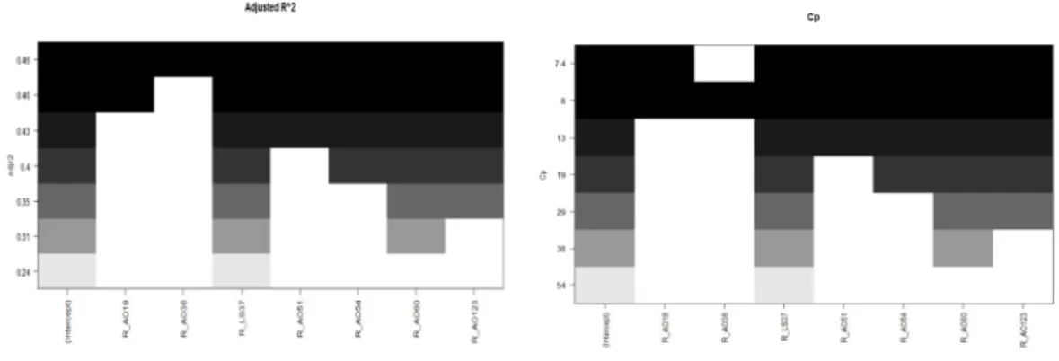
Aside from information criteria, another way to check the importance of each variable is with a graphical representation of each model and its importance over the model adjusted R2 and Mallow’s Cp. Each row represents a model and each dark colored block represents the inclusion of such

variable in the model. The objective is the find a model that maximizes R2 and minimizes Cp. A

variable that is more persistent over the various models should be preferred over a less persistent one.

Figure 17 – Subset Model diagrams – Adjusted R2 and Mallow’s Cp for Total Sales

Having in account the various criteria for variable selection, the best overall variables are comprised in the follow regression equation.

yt = β0 + β1 AO18t + β2 AO51t + β3 AO54t + β4 AO60t + β5 AO123t + ϵt (2)

β sβ t value Pr(>|t|) Significance β0 16943,4 487,3 34,793 2,00E-16 *** AO18 17159,0 5401,1 3,177 1,89E-03 ** AO51 10776,1 5401,5 1,995 4,83E-02 * AO54 13134,5 5401,3 2,432 1,65E-02 * AO60 16938,7 5401,7 3,136 2,15E-03 ** AO123 13334,5 5401,2 2,469 1,50E-02 *

20 Once the regression model has been selected, it is estimated the orders of the ARIMA parameters, this time regarding the residuals of the regression model, and subsequently calculated the various permutations around the preliminary parameters.

Table 6 – ARIMA models overview – Total Sales with outliers

This development has conducted into better accuracy results compared to the first ARIMA estimation, without outliers.

4.4. F

T

S

E

F

To have a better understanding on the influences of external factors over Portuguese vehicle sales, it was applied cross-correlation function to determine if there is any relationship at a lagged time and thus see it is a useful predictor of sales.

Since the direct application of CCF methodologies are affected by the time series structures and any “in common” trends that both series may have over time. It was needed to apply methodologies to minimize these disturbances such as pre-whitening.

As consequence of this process, the correlation values become much more subtle, without any high correlation values, which imply a much more careful observation and choice to not be confounded with not correlated factors.

21

4.4.1. Factors with some evidence of Correlation

From the various factors analysed, the ones that has shown higher correlation value (positive correlation in grades of red, negative correlation in grades of blue) are summarized below.

Factors Lags t-12 t-11 t-10 t-9 t-8 t-7 t-6 t-5 t-4 t-3 t-2 t-1 t R1 0,06 -0,02 -0,09 -0,07 -0,05 -0,26 -0,21 -0,11 -0,22 -0,24 -0,27 -0,09 -0,1 R2 -0,22 -0,11 -0,05 -0,01 0,04 0,02 0,04 0,04 0,08 0,14 0,21 0,25 0,24 R3 -0,03 -0,03 0,06 0,11 0,12 0,04 -0,06 -0,02 0,01 0,17 0,18 0,22 0,27 R4 0,06 -0,07 -0,02 0,15 -0,08 -0,11 0,04 0,07 -0,02 -0,06 0,01 -0,17 -0,25 R5 -0,19 0 -0,11 -0,09 0,04 0,12 -0,01 -0,21 -0,19 0,06 -0,04 0,04 0,17 R6 -0,03 0,01 -0,01 -0,16 -0,06 0,06 -0,06 0,04 0,11 -0,01 0,11 0,06 -0,24 R7 0,04 -0,03 -0,11 -0,28 -0,05 -0,02 -0,09 -0,01 0,11 0,13 0,03 0,02 -0,08 R10 -0,09 0,09 -0,03 -0,02 0,01 0,05 -0,05 -0,21 -0,2 0,08 0,09 0,25 0,16 R11 -0,14 0,01 0,00 -0,01 -0,03 0,02 0,2 0,15 0,18 0,28 0,33 0,33 0,22 R15 -0,05 0,12 -0,08 -0,05 0,08 0,01 0,05 -0,19 -0,04 -0,01 0,06 -0,09 0,2 R16 -0,1 0,1 -0,08 0,07 0,18 -0,13 -0,04 -0,03 -0,05 -0,06 0,09 -0,03 0,04 R17 0,01 0,07 0,11 0,11 0,1 -0,07 -0,08 -0,01 -0,08 0,19 0,05 0,35 0,05 R18 0,11 -0,08 0,20 -0,11 -0,07 0,01 0,04 -0,12 0,10 0,06 -0,11 -0,05 0,21 R19 -0,03 0,13 -0,28 0,13 0,10 -0,13 0,06 0,10 -0,17 0,10 0,04 -0,21 0,18

R1 - Unemployment rate; R2 - Private Consumption Indicator; R3 - Economic Climate Indicator; R4 - Expectations of unemployment over next 12 months; R5 - Expectations on economic

climate over the next 12 months; R6 - Consumer price index; R7 - Crude Oil price; R10 - Appreciation on economic climate of the last 12 months; R11 - Economic Activity Indicator; R15 - Savings Opportunity; R16 - Expectation of equipment good acquisition in the next 12 months; R17 - Expectation on sales prices over the next 3 months; R18 - Number of weekday holidays per month; R19 - Number of workdays per month

Figure 18 – Cross Correlation table – Total Sales

Observing the different factors, it is interesting to note that most of these are factors that indicate the economic status of the country. The only social factor present in unemployment rate which is most correlated at lag 2. Also to be noted is how oil prices affect vehicle sales 9 months earlier.

4.4.2. Spurious Correlations

While analysing the CCF table, there are some factors featured as high positive correlative values such as R17 - expectations on sales prices. Intuitively and empirically it is not expected for automotive sales to go up when sales prices are going up, therefore this correlation will be considered as spurious.

22

4.5. M

F

R

A

E

From the factors that has shown the highest correlation, a regression model was created using them as predictors at respective lags.

β sβ t value Pr(>|t|) Significance β0 68102,6 146393,4 0,465 6,43E-01 R1_lag7 -7874,1 2630,0 -2,994 3,49E-03 ** R2_lag1 353,0 145,4 2,427 1,70E-02 * R3_lag1 270,8 440,9 0,614 5,40E-01 R4_lag0 4333,7 3579,3 1,211 2,29E-01 R5_lag3 14651,3 13104,1 1,118 2,66E-01 R6_lag0 9,2 3,1 2,986 3,58E-03 ** R7_lag9 -60,3 20,0 -3,015 3,28E-03 ** R10_lag1 12718,2 12995,9 0,979 3,30E-01 R11_lag2 117405,1 216340,5 0,543 5,89E-01 R15_lag0 28627,5 22800,2 1,256 2,12E-01 R16_lag8 27633,1 24106,2 1,146 2,54E-01 R18_lag0 701,8 432,2 1,624 1,08E-01 R19_lag0 15,5 14,0 1,109 2,70E-01 AO18 12758,0 3264,6 3,908 1,72E-04 *** AO36 3090,4 3348,5 0,923 3,58E-01 LS37 -2000,8 1300,5 -1,538 1,27E-01 AO51 8248,1 3281,9 2,513 1,36E-02 * AO54 10260,9 3215,9 3,191 1,91E-03 ** AO60 14439,2 3351,8 4,308 3,95E-05 *** AO123 9351,3 3256,2 2,872 5,01E-03 **

Table 7 –Regression coefficients – Total Sales with outliers and external factors

From this initial regression equation, it is possible to see that many on these factors are not significant for the model.

23 β sβ t value Pr(>|t|) Significance β0 40481,1 20169,4 2,007 4,98E-02 * R1_lag7 -11496,2 2635,7 -4,362 3,05E-05 *** R3_lag1 1682,9 294,7 5,711 1,07E-07 *** R4_lag0 10708,4 2827,1 3,788 2,55E-04 *** R6_lag0 7,2 2,2 3,301 1,32E-03 ** R7_lag9 -82,4 19,0 -4,339 3,32E-05 *** R16_lag8 55650,2 21655,1 2,570 1,16E-02 * AO18 10997,7 3052,4 3,603 4,84E-04 *** AO36 6078,1 3063,4 1,984 4,99E-02 * AO51 8375,3 3041,1 2,754 6,95E-03 ** AO54 11594,0 3014,1 3,847 2,07E-04 *** AO60 16685,7 3032,8 5,502 2,71E-07 *** AO123 10191,6 3087,1 3,301 1,32E-03 **

Table 8 –Final Regression coefficients – Total Sales with outliers and external factors

yt = β0 + β1 R1t-7 + β2 R3t-1 + β3 R4t + β4 R6t + β5 R7t-9 + β6 R16t-8 + β7 AO18t +β8 AO36 t +

β9AO51 t + β10 AO54 t + β11 AO60 t + β12 AO123 t + ϵt ₍₃₎

From this general model it is possible to observe the inverse relationship towards employment rates and oil prices; and the direct relationship on economic climate, employment expectations of the following year and expectation on equipment acquisition. There is also some effect on consumer prices but its effect is very small when compared with other factors. This may be due to the slow changing behaviour of this factor. The model above was used to create the forecasting model and was chosen the top 10 models that minimized the Akaike Information Criteria and sorted by lowest MAPE.

Table 9 – ARIMA models overview – Total Sales with outliers and external factors

Through the analysis of the previous table it can be observed that there is an increase in accuracy compared with both previous models.

24

5. HIERARCHICAL FORECASTING - VEHICLE MARKET AS A SUM OF PARTS

To test the initial hypothesis that forecasting multiple subsets of the data has better accuracy than forecasting the data as a whole; this chapter will focus on the analysis of different segments of the automotive market.

5.1. F

T

S

L

H

:

C

R

+

F

M

The first level split to be analysed will be between Car Rental vehicle acquisition and the Free Market which is comprised by the general public and companies.

Figure 20 – One level hierarchical forecasting: Car Rental + Free Market

5.1.1. Forecasting Car Rental

As commented in the first chapter, Portuguese car rental market represents 20% of the total market and over the years has shown a rather coherent and predictable seasonality. Such behaviour can be favourable for forecasting models as its accuracy should be much higher.

25

Figure 22 – Outlier detection – Car Rental

Date Type Observations

AO51 Mar 2010 Additive Tax incentive to end-of-life

vehicle on April 2010

Table 10 – Outliers – Car Rental

Regarding major outliers, the only significant outlier detected coincides with the government announcement of tax incentives to end-to-life vehicles. This market normally is a high volume fleet acquisition with established contracts and dates so it is to be expected not to have any major and unexpected fluctuations as with the general public.

Best regression model with outliers

yt = β0 + β1 AO51t + ϵt (4)

β sβ t value Pr(>|t|) Significance

β0 2592,7 178,8 14,502 2,00E-16 ***

AO51 4267,3 2014,8 2,118 3,62E-02 *

Table 11 – Regression model - Car Rental with outliers

Regarding to external factors, the ones that show higher correlation are in fact the ones related with tourism anddemand on service activities.

26

External Factor Evaluation

Factors Lags t-12 t-11 t-10 t-9 t-8 t-7 t-6 t-5 t-4 t-3 t-2 t-1 t R8 0,00 -0,14 -0,06 -0,17 -0,10 -0,07 -0,05 0,06 0,16 0,20 0,32 0,19 0,12 R9 0,08 -0,03 -0,02 -0,20 -0,22 -0,10 -0,17 0,00 0,14 0,23 0,28 0,15 0,19 R20 -0,08 -0,10 -0,07 0,00 -0,03 -0,02 0,00 -0,04 0,09 0,15 0,25 0,37 0,32

R8 - Nights spent at tourist accommodation establishments – Residents; R9 - Nights spent at tourist accommodation establishments - Non-Residents; R20 – Expectations on demand on

services over the next 3 months

Table 12 – Cross Correlation table – Car Rental

It is interesting to observe that the tourism anticipates sales of car rental, especially resident tourists. Quite possibly it refers to sales of next touristic season and not direct reaction of the increase in tourism rate. More interesting is the expectation on the increase of activity in the service sector and vehicle acquisition may be a way of preparation for this expected increase. There is no evidence any social factors correlated with this data.

Best regression model with outliers and external factors

yt = β0 + β1 R8t-2 + β2 R20t-1 + β3 AO51 t + ϵt (5) β sβ t value Pr(>|t|) Significance β0 -19115,3 8821,1 -2,167 3,22E-02 * R8_lag2 3479,7 1122,6 3,100 2,41E-03 ** R20_lag1 6726,9 540,2 12,453 2,00E-16 *** AO51 3410,3 1365,3 2,498 1,38E-02 *

Table 13 – Regression model - Car Rental with outliers and external factors

It would be expected that non-resident tourism would have higher impact on car rental sales but is actually the residents that are significant.

Forecast Evaluation

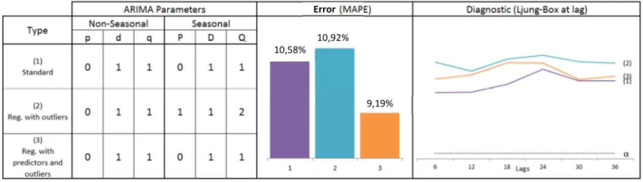
Below are summarized the three best models of each criterion: standard ARIMA, regression model with ARIMA errors with outliers as predictors and regression model with ARIMA errors with outliers and external factors as predictors.

27

Table 14 – ARIMA models overview – Car Rental

From these three models the one with external factors show higher accuracy.

5.1.2. Forecasting Free Market

The free market, comprised the general public and enterprises, normally does not have scheduled planning as the car rental agreements so its trends tend to be much more unexpected and therefore more difficult to forecast.

Figure 23 – Free Market time series Figure 24 – Outlier detection – Free Market

Date Type Observations

AO18 Jun 2007 Additive Changes on CO2 emission tax + Increase

on vehicle tax on July 2007

AO31 Jul 2008 Additive VAT decrease from 21% to 20% on July

2008

AO36 Dec 2008 Additive Alteration over CO2 emission tax on

January 2009

LS37 Jan 2009 Level Shift Alteration over CO2 emission tax

AO60 Dec 2010 Additive VAT increase from 21% to 23% on Jan

2011

LS64 Apr 2011 Level Shift Portugal announces arrangement for

monetary aid from IMF

AO72 Dec 2011 Additive Increase on vehicle tax on Jan 2012

AO123 Mar 2016 Additive Increase on vehicle tax on April 2016

Table 15 – Outliers – Free Market

10,58% 10,92%

9,19%

Error

28 Through the outlier detection it is possible to observe that the general public is much more susceptible to announcements and changes of economic policies. As appeared in the outlier detection of the total sales data, every time there would be an increase on taxes, the previous month is subjected to an overgrowth in sales. It is also interesting in this series the capture of other outliers such as decrease of taxes and specially, in April 2011, the coincidence with the announcement of the monetary aid from IMF. This surely implies that any major economic news is indeed influencer of vehicle sales.

Best regression model with outliers

yt = β0 + β1 AO18t + β2 AO36 t + β3 LS37 t + β4 AO60 t + β5 LS64 t + β6 AO123 t + ϵt (6)

β sβ t value Pr(>|t|) Significance β0 19710,5 511,0 38,574 2,00E-16 *** AO18 11613,5 3023,0 3,842 1,97E-04 *** AO36 6633,5 3023,0 2,194 3,01E-02 * LS37 -3547,4 776,2 -4,570 1,19E-05 *** AO60 15250,9 3036,3 5,023 1,79E-06 *** LS64 -5271,0 694,5 -7,589 7,64E-12 *** AO123 13003,9 3003,1 4,330 3,11E-05 ***

Table 16 – Regression model – Free Market with outliers

External Factor evaluation

Taking in consideration external factor contribution, the ones that have major effect over the free market as described on the following table.

Factors Lags t-12 t-11 t-10 t-9 t-8 t-7 t-6 t-5 t-4 t-3 t-2 t-1 t R1 -0,07 -0,04 0,00 -0,06 -0,19 -0,32 -0,29 -0,22 -0,23 -0,22 -0,26 -0,19 -0,11 R2 -0,24 -0,18 -0,14 -0,09 -0,03 0,00 0,05 0,07 0,13 0,17 0,22 0,26 0,25 R11 -0,16 -0,02 -0,04 -0,02 0,02 0,08 0,19 0,19 0,23 0,31 0,35 0,32 0,28 R14 0,05 0,01 0,02 0,10 0,15 0,20 0,24 0,32 0,23 0,12 0,04 -0,01 0,11 R24 0,26 -0,05 -0,25 0,04 0,07 0,11 0,23 0,14 -0,18 -0,24 -0,02 0,20 0,32

R1 - Unemployment rate; R2 - Private Consumption Indicator; R11 - Economic Activity Indicator; R14 - Employment Index on Service Sector; R24 – Salary index on Service Sector

Table 17 – Cross Correlation table – Free Market

Best regression model with outliers and external factors

29 β sβ t value Pr(>|t|) Significance β0 _{-15710,0 2443,0 -6,433 3,04E-09 ***} R2_lag1 457,3 38,6 11,836 2,00E-16 *** AO18 12150,0 2492,0 4,878 3,51E-06 *** AO60 15750,0 2478,0 6,354 4,45E-09 *** AO72 7252,0 2540,0 2,855 5,12E-03 ** AO123 10250,0 2487,0 4,121 7,18E-05 ***

Table 18 – Regression model – Free Market with outliers and external factors

For the model above, the factor that influences the most is the private consumption indicator in a positive relationship.

Forecast Evaluation

Table 19 – ARIMA models overview – Free Market

As expected, there is an increase of accuracy when adding outliers and, furthermore, when adding external factors, even though very slightly. Analyzing the error itself, it was expected to be higher that car rental. Also it has to be considered that the Free Market series is comprised by two subsets, passenger and commercial, with different behaviors.

5.1.3. Results

Table 20 – Forecast aggregation: Car Rental + Free Market

16,13% 11,52% 10,93% Error horizon t-3 t-2 t-1 t

30 Aggregating the best forecasting models for car rental and free market into a one level hierarchy has a MAPE of 8,029% which is slightly better when compared with the original forecast on vehicle sales as a whole.

5.2. F

T

S

O

L

H

:

P

+

C

Another type of hierarchical split that can be analysed is, naturally, between passenger and commercial vehicles. Passenger vehicles are normally associated with the general public while commercial with business to business acquisitions and both are expected to have different trends.

Figure 25 – One level hierarchical forecasting: Passenger + Commercial vehicles

5.2.1. Forecasting Passenger Market

Passenger marker is comprised by approximately 80% of total vehicle sales and, as mentioned before, targets the public in general. In the latter years there has been an upward trend in sales with consistent seasonal behaviour which will favour the forecast models.

Figure 26 – Passenger Market time series

Figure 27 – Outlier detection – Passenger Market

31

Date Type Observations

AO36 Dec 2008 Additive Increase over CO2 emission tax on

January 2009

LS37 Jan 2009 Level Shift Increase over CO2 emission tax

AO51 Mar 2010 Additive Tax incentive to end-of-life vehicle on

April 2010

AO54 Jun 2010 Additive VAT increase from 20% to 21% on July

2010

AO60 Dec 2010 Additive VAT increase from 21% to 23% on Jan

2011

AO123 Mar 2016 Additive Increase on vehicle tax on April 2016

Table 21 – Outliers – Passenger Market

From the outliers detection it is also clear that passenger vehicle sales are sensitive to vehicle taxation and incentives. These outliers are similar from the ones that were captured previously.

Best regression model with outliers

yt = β0 + β1 LS37 t + β2 AO51t + β3 AO54 t + β4 AO60 t + β5 AO123t + ϵt (8)

β sβ t value Pr(>|t|) Significance β0 16941,9 641,2 26,421 2,00E-16 *** LS37 -4409,2 762,4 -5,783 5,86E-08 *** AO51 11303,4 3869,4 2,921 4,16E-03 ** AO54 13496,4 3869,4 3,488 6,79E-04 *** AO60 15585,4 3869,4 4,028 9,86E-05 *** AO123 13926,4 3869,4 3,599 4,64E-04 ***

Table 22 – Regression model – Passenger Market with outliers

External Factor evaluation

Factors Lags t-12 t-11 t-10 t-9 t-8 t-7 t-6 t-5 t-4 t-3 t-2 t-1 t R1 0,02 -0,04 -0,09 -0,07 -0,07 -0,31 -0,20 -0,15 -0,23 -0,24 -0,29 -0,12 -0,09 R3 -0,04 -0,02 0,06 0,10 0,10 0,02 -0,03 0,00 0,08 0,21 0,26 0,26 0,32 R18 0,11 -0,08 0,20 -0,11 -0,07 0,01 0,04 -0,12 0,10 0,06 -0,11 -0,05 0,21

R1 - Unemployment rate; R3 -Economic Climate Indicator; R18 – Number of weekday holidays per month

Table 23 – Cross Correlation table – Passenger Market

Best regression model with outliers and external factors

yt = β0 + β1 R3t-1 + β2 R18 t + β3 AO51t + β4 AO54 t + β5 AO60 t + β6 AO123 t + ϵt

32 β sβ t value Pr(>|t|) Significance β0 38818,1 6062,4 6,403 3,77E-09 *** R3_lag1 871,9 137,0 6,366 4,50E-09 *** R18_lag0 720,4 326,4 2,207 2,94E-02 * AO51 8883,9 3053,0 2,910 4,37E-03 ** AO54 10380,9 3054,0 3,399 9,40E-04 *** AO60 12526,6 3053,6 4,102 7,83E-05 *** AO123 11447,1 3031,9 3,776 2,58E-04 ***

Table 24 – Regression model – Passenger Market with outliers and external factors

From this model, it seems that even though unemployment rate is positively correlated with passenger vehicle sales, it was not significant for the regression model, which can be concluded that passenger market is mainly influenced by economic factors.

Forecast Evaluation

Table 25 – ARIMA models overview – Passenger Market

From this summary of models, similar deduction as the previous models can be extracted. Models with outliers and external factors tend to have higher accuracy than a standard ARIMA approach.

5.2.2. Forecasting Commercial Market

Commercial market complements the previous study, with 20% of the total market.

Figure 28 – Commercial Market time series Figure 29 – Outlier detection – Commercial Market

13,71%

9,10% _8,65%

Error

33

Date Type Observations

TC15 Mar 2007 Temp. Change

TC17 May 2007 Temp. Change Antecipation on tax increase

AO18 Jun 2007 Additive

Increase on CO2 emission tax + Increase on vehicle tax on July 2007

LS37 Jan 2009 Level Shift Alteration over CO2 emission tax

AO60 Dec 2010 Additive VAT increase from 21% to 23% on

Jan 2011

AO72 Dec 2011 Additive Increase on vehicle tax on Jan

2012

LS74 Fev 2012 Level Shift

AO96 Dec 2013 Additive

AO123 Mar 2016 Additive Increase on vehicle tax on April

2016

Table 26 – Outliers – Commercial Market

Again, most of the outliers detected are influenced by economic events.

Best regression model with outliers

yt = β0 + β1 AO18 t + β2 LS37 t + β3 AO60t + β4 AO72 t + β5 LS74t + β6 AO123t + ϵt (10)

β sβ t value Pr(>|t|) Significance β0 5063,8 130,4 38,831 2,00E-16 *** AO18 6016,2 782,4 7,689 4,54E-12 *** LS37 -1912,2 184,4 -10,369 2,00E-16 *** AO60 2611,4 782,4 3,338 1,13E-03 ** AO72 2358,4 782,4 3,014 3,14E-03 ** LS74 -1175,7 168,0 -6,997 1,61E-10 *** AO123 1842,1 778,7 2,366 1,96E-02 *

Table 27 – Regression model – Commercial Market with outliers

On the analysis of cross-correlations with the different external factors, it was found that there was no significant correlation with any factor which implies that the outlier analysis is rather enough or there were other external factors that were not taken in account. Having in account the accuracy of the prediction model using only outliers, it can be considered that this model is rather good and viable.

34

Forecast Evaluation

Table 28 – ARIMA models overview – Commercial Market

Having a more predictable behavior, the forecasting accuracy has greatly increased when compared with the previous subsets.

5.2.3. Results

Table 29 – Forecast aggregation: Passenger + Commercial Market

Compared with the previous hierarchical aggregation, this one provides a better average accuracy. Partially due to Free Market encompassing two different behaviors, which in this model are separated. In the light of this information it is compelling to determine if car rental separated from the passenger and commercial market would bring even better results.

8,29% 5,48% Error t-3 t-2 t-1 t horizon

35

5.3.

F

T

S

L

H

To further enhance the study, it will be analyzed if a two level hierarchy will bring significant accuracy improvement when compared with the previous models. For the second level split it will be considered between passenger car rental and passenger free market as an attempt of bringing together the knowledge acquired before. From the commercial category, there is no significant sales on car rental, thus it will be considered the same model as previously.

Figure 30 – Two levels hierarchical forecasting

5.3.1. Forecasting Passenger Car Rental

From the car rental standpoint, passenger vehicles comprise the majority of the sales, so it is expected for this subset to behave in terms of forecasting to the car rental market.

Figure 31 – Passenger Car Rental time series

Figure 32 – Outlier detection – Passenger Car Rental

36

Date Type Observations

AO54 Jun 2010 Additive VAT increase from 20% to 21%

on July 2010

LS100 Apr 2014 Level Shift

Table 30 – Outliers – Passenger Car Rental

Best regression model with outliers

yt = β0 + β1 AO54 t + β2 LS100t + ϵt (11)

β sβ t value Pr(>|t|) Significance

β0 1979,3 178,3 11,101 2,00E-16 ***

AO54 5911,7 1774,1 3,332 1,14E-03 **

LS100 1613,8 378,2 4,267 3,90E-05 ***

Table 31 – Regression model – Passenger Car Rental with outliers

As the data is subset further and further, there are less outliers detected that have significant impact over the series.

External Factor evaluation

Factors

Lags

t-12 t-11 t-10 t-9 t-8 t-7 t-6 t-5 t-4 t-3 t-2 t-1 t

R8 0,01 -0,14 -0,06 -0,18 -0,10 -0,07 -0,04 0,06 0,15 0,20 0,32 0,20 0,12

R8 – Nights spent at tourist accommodation establishments - Residents

Table 32 – Cross Correlation table – Passenger Car Rental

Best regression model with outliers and external factors

yt = β0 + β1 R8t-2 + β2 AO54 + β3 LS100t + ϵt (12) β sβ t value Pr(>|t|) Significance β0 150,9 13,4 11,287 2,00E-16 *** R8_lag2 -0,1 0,0 -5,460 2,58E-07 *** AO54 97,0 34,7 2,794 6,05E-03 ** LS100 35,9 7,4 4,837 3,92E-06 ***

37

Table 34 – ARIMA models overview – Passenger Car Rental

As expected, the forecast accuracy is very high when forecasting with the regression aggregated with outliers and external factors.

5.3.2. Forecasting Passenger Free Market

The Passenger free market has the biggest weight in this split, in terms of volume, and also has the less consistent behavior, so it would be expected to have lower prediction accuracy.

Figure 33 – Passenger Free Market time series Figure 34 – Outlier detection – Passenger Free Market

Date Type Observations

AO18 Jun 2007 Additive

Increase on CO2 emission tax + Increase on vehicle tax on July 2007

AO36 Dec 2008 Additive Increase over CO2 emission tax on

January 2009

LS37 Jan 2009 Level Shift Increase over CO2 emission tax

LS44 Aug 2009 Level Shift

TC59 Nov 2011 Temp. Change Antecipation on VAT increase

AO60 Dec 2011 Additive VAT increase from 21% to 23% on

Jan 2011

AO123 Mar 2016 Additive Changes on vehicle tax on April

2016

Table 35 – Outliers – Passenger Free Market

11,10%

6,31%

3,31%

Error