RBRH, Porto Alegre, v. 23, e52, 2018 Scientific/Technical Article
https://doi.org/10.1590/2318-0331.231820180013
Manning’s roughness coefficient for the Doce River
Coeficiente de rugosidade de Manning para o Rio Doce
Emmanuel Kennedy da Costa Teixeira1, Márcia Maria Lara Pinto Coelho2, Eber José de Andrade Pinto2,
Jéssica Guimarães Diniz1 and Aloysio Portugal Maia Saliba2
1Universidade Federal de São João del-Rei, Ouro Branco, MG, Brasil 2Universidade Federal Minas Gerais, Belo Horizonte, MG, Brasil
E-mails: [email protected] (EKCT), [email protected] (MMLPC), [email protected] (EJAP), [email protected] (JGD), [email protected] (APMS)
Received: January 31, 2018 - Revised: July 25, 2018 - Accepted: September 11, 2018
ABSTRACT
The Manning’s roughness coefficient is used for various hydraulic modeling. However, the decision on what value to adopt is a complex task, especially when dealing with natural water courses due to the various factors that affect this coefficient. For this reason,
most of the studies carried out on the subject adopt a local approach, such as this proposal for the Doce River. Due to the regional
importance of this river in Brazil, the objective of this article was to estimate the roughness coefficient of Manning along the river, in
order to aid in hydraulic simulations, as well as to discuss the uncertainties and variations associated with this value. For this purpose,
information on flow rates and water depths were collected at river flow stations along the river. With this information, the coefficients
were calculated using the Manning equation, using the software Canal, and their space-time variations were observed. In addition, it
was observed that the uncertainties in flow and depth measurements affect the value of the Manning coefficient in the case studied.
Keywords: Uncertainties in the roughness coefficient; Hydraulic modeling; Monte Carlo simulation.
RESUMO
O coeficiente de rugosidade Manning é utilizado em várias modelagens hidráulicas. Entretanto, a decisão sobre qual valor será adotado é uma tarefa complexa, principalmente se tratando de cursos d’água naturais, devido aos vários fatores que afetam esse coeficiente.
Por isso, na maioria dos estudos realizados sobre o tema se adota uma abordagem local, como a proposta para o Rio Doce. Devido à importância regional deste rio no Brasil, o objetivo deste artigo foi estimar a rugosidade de Manning ao longo do Rio Doce, de forma
a auxiliar em simulações hidráulicas, e também discutir as incertezas e as variações associadas a esse valor. Para isso, foram levantadas informações de vazões e profundidades da água em estações fluviométricas ao longo do rio. De posse dessas informações, calcularam‑se
os referidos coeficientes utilizando‑se a equação de Manning, sendo que para isso utilizou‑se o software Canal, e foram observadas suas
variações espaço‑temporal. Além disso, foi observado como as incertezas nas medições de vazões e de profundidades afetam o valor do coeficiente de Manning no caso estudado.
INTRODUCTION
One of the most widely used equations for calculating
the flow rate in open channel in uniform flow is Manning’s
(PARSAIE et al., 2017). This expression defines the balance
between motive force (gravity) and the flow resistance, being this resistance expressed through Manning’s roughness coefficient “n”.
This roughness coefficient is commonly used in numerical
modelings to study rivers hydraulic behavior (KIM et al., 2013),
as well as to generate simulations in order to construct flooding
maps, hydraulic structures projects, like bridges and dams, among other applications. Kopecki, Schneider and Tuhtan (2017) presents that regardless the dimensionality (1D, 2D, etc) of the hydraulic model used, all of them must be calibrated adjusting one value to
the Manning’s coefficient, in order to reproduce the water surface elevations that have a close value to the field measurements.
However, the adoption of an appropriate coefficient can
be challenging, involving practical experience and individual and local judgements, which could result in obtaining different values in the analysis of the same channel (ZINK; JENNINGS, 2014; AYVAZ, 2013). This happens due to the fact that the roughness
coefficient has its value influenced by numerous factors, since the flow of the rivers happens in diverse and complex conditions
(FARD; HEIDARNEJAD; ZOHRABI, 2013; CALO et al., 2013).
Chow (1959) presents that various interfering factors can affect the
coefficient, such as the surface roughness, channel irregularities
and alignment, vegetation effects, changes on the channel bed geomorphology due to deposit or degradation of materials and the transport of suspended and/or bottom sediments. In addition,
the author presents that the roughness coefficient varies in the
cross section due to the variation in water levels, the lower the
water depth, the higher the coefficient value, since the effects of
the irregularities of the canal bottom are more evident.
Nimnim and Farhan (2015) presented that the roughness
coefficient also varies due to the bottom slope of the channel. That is why they varied the flow rate and the bottom slope of
trapezoidal and semicircular canals, which were built in the laboratory.
The slopes tested were 0.002, 0.003 and 0.004 m/m. For each slope, the flow rate varied between 2 and 10 L/s, obtaining the variation of the roughness coefficient, which was always around 5% for
the three slopes, that is, the differences between the roughnesses
for the flows of 2 to 10 L/s were approximately 5%.
Due to the importance and the difficulty in determining the roughness coefficient, several authors presented equations
to quantify this value, which are presented in the specialized literature. Prajapati, Vadher and Yadav (2016) found roughness
coefficients using Manning’s Equation, the empirical relations of
Limerinous, Strickler, Meyer-Peter and Muller and from the Cowan table. The results were compared to the value observed at the Garudeshwar station in the Purna River, in India. They concluded
that the roughness coefficient calculated through Manning’s
equation is the one closest to the one observed, with an error of almost zero percent.
In the literature, there are softwares that calculate the
roughness coefficient from the Manning equation. One of them is
the program Canal (PRUSKI et al., 2006), which was developed by
the Research Group on Water Resources of the Federal University
of Viçosa (UFV, 2018), and used in this work, as will be explained in the following item.
In addition to the classical methods, in the present days, some authors have proposed other means to determine the roughness
coefficient. Mtamba et al. (2015) used Radarsat-2 and Landsat TM
for spatial estimation of Manning’s roughness coefficient. Using
the FLO-2D hydrodynamic model, the authors compared the
water level found when using the roughness coefficient obtained with field information, to the one obtained using the roughness
estimated from images, being that the two methods presented similar results.
However, even with the recent and old methodologies,
uncertainties remain in estimating the roughness coefficient, since
methods were developed according to local characteristics and may
not fit other situations. Therefore, it is important that research at
local levels, as proposed here, continue to be developed, in order to assist in hydraulic modeling. Therefore, several authors researched
the behavior of the local roughness coefficient.
Zink and Jennings (2014) estimated the roughness coefficient
in mountain rivers in North Carolina. Fard, Heidarnejad and Zohrabi (2013) determined an equation for the roughness coefficient of the Karum River. Parhi, Sankhua and Roy (2012) calibrated the
value of the Manning coefficient to the Mahanadi River through flood simulation using the Hydrologic Engineering Center’s
River Analysis System (HEC-RAS). Matos et al. (2011) based their research on theoretical and practical studies to determine
the roughness coefficient of the Sapucaí River in Minas Gerais.
Lyra et al. (2010) determined the roughness coefficient for the Paracatu River as a function of the geometric characteristics of
the channel and the series of daily flow rates from river stations
existing along the river.
Other authors besides estimating the Manning’s coefficient,
also promoted discussion about the uncertainty associated to
it. Kim, Kim and Woo (1995) presented the range of the Han
River roughness coefficient and showed that a 20% change in its value can cause the calculated flood peak to vary by up to
10%. Kim et al. (2010) show that due to errors of measuring
water flow and water depth, the estimated roughness coefficient based on field data presents uncertainties. Using the Monte Carlo
simulation, the authors determined the variation of the roughness
coefficient when there is a variation of 5 and 10% in the flow rate, with a roughness variation of 6 to 14%. In addition, for the
roughness values obtained via Monte Carlo, they observed how this uncertainty impacts the values of estimated depths, obtaining
a variation of approximately 2 to 4%. Golshan, Jahanshahi and
Afzali (2016) defined the flood areas for the return periods of 2, 5, 10, 25, 50, 100 and 200 years for the Safarood drainage basin, using HEC-RAS. By doubling the value of the roughness
coefficient, the authors obtained that, for the periods of return from 2 to 200 years, the flood zone increased by 8.8% to 15.7%,
respectively.
A river of great importance in the national scenario is the Doce, also, there are several hydroelectric projects, from which, at the moment, four of them are hydroelectric plants (UHE) of greater size, and there are plans to install three more. It occurs that during the design and operation phases of these UHEs, numerical modeling is necessary for predictions of the behavior of the water line and the silting process of the reservoir. For cities with
flooding problems, hydraulic simulations are also needed, such
flood spots for parts of the Doce River located in Governador
Valadares-MG and Colatina-ES, respectively.
To implement these modelings one of the necessary input
parameters is the Manning coefficient. However, there are no studies
in the literature that have proposed to study the range of values and the behavior of Manning for this river. Therefore, studies such as the one proposed here are needed, so it can assist in future hydraulic simulations. The objective of this article is, therefore, to estimate the Manning’s roughness along the Doce River, in order to compose a database that can help in future hydraulic simulations. In addition, it is discussed how the uncertainties in
the Manning value can influence the final result of a hydraulic
simulation, being also presented the spatio-temporal variations
that occur with this coefficient.
MATERIAL AND METHODS Study area
The Doce River drainage basin covers a total of 230 municipalities, in which more than 3.5 million inhabitants
live. It has a drainage area of approximately 83,400 km2, with 86%
of the basin being in Minas Gerais (MG) and 14% in the state
of Espírito Santo (ES) (CBH-DOCE, 2013). Located between
the parallels 17º45 ‘and 21º15’S and the meridians 39º30’ and 43º45’W, the basin integrates the hydrographic region of the
Southeast Atlantic.
Its main river is the Doce, and its springs are found in the mountains of Mantiqueira and Espinhaço, in MG. Its formation takes place through the meeting of the Piranga River with Ribeirão
do Carmo. It is approximately 850 km long and flows into the
Atlantic Ocean, in Regência, ES (CBH-DOCE, 2013).
A characteristic that allows the determination of the values of Manning for the Doce River is the fact that, along the river,
there are river flow stations that have historical series with the necessary data for the calculation of this coefficient. As described
next, seven stations were used, which are distributed along the extension of 525 km of the river.
Determination of Manning’s roughness along the Doce River
When making hydraulic simulations, the values of the Manning’s roughness coefficient “n” are required. Therefore, in order to estimate these values along the Doce River, the river flow
stations that presented data series of cross‑section, daily “Q” flows and water level quotas were surveyed on the HidroWeb website of the National Water Agency (ANA), and from the differences
between the water levels and the smallest quotas of each cross
section, the water depths “y” were obtained. Seven stations were
found, which are presented in Table 1 and in Figure 1.
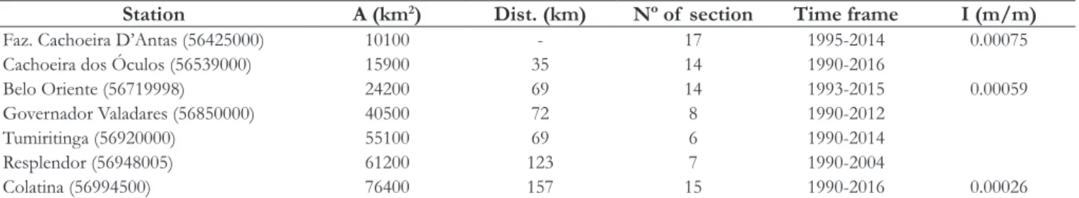
Table 1 shows the drainage area (A) for the seven river
flow stations, the distances between one station and the next, the
number of cross sections of each station, the period comprised of the measurements and the average slope.
The cross sections were surveyed only one time per year, not necessarily every year, which explains why section numbers differ between stations and why they are different from the number of years in the analyzed period. For example, for the station 56920000
there are cross section profiles comprised between 1990 and 2014
(Table 1). However, in this period only six sections were surveyed,
which are from 1990, 1996, 2011, 2012, 2013 and 2014.
It should be emphasized that there is no specific month
to carry out the surveys, so, there are cross sections obtained for months that vary from April to November, and there is no
station that has a cross section profile surveyed from December to March, which are the main months for floods.
As done in Lyra et al. (2010) and Golshan, Jahanshahi and Afzali (2016), the slope of the water line was considered
approximate to the slope “I” of the bottom of the river. According
to CBH-DOCE (2005), the approximate mean slopes of the main channel of the river are 0.00075 m/m at the high, 0.00059 m/m at the medium and 0.00026 m/m at the low Doce. These slopes were attributed to the stretches where the cross sections presented in Table 1 are, according to the location of the station.
For each cross section profile and the values of “Q” and “y” measured on the day of the section survey, the values of “n” were
calculated using the Manning equation, with the assistance of the
software Canal. Thus, for each river flow station an amount of “n” values equal to the number of cross sections was obtained.
The software Canal uses the Manning equation (Equation 1) for the design of open channels. One must enter the slope of the river stretch, the coordinates of the cross-sections of interest, and, from the water depth value informed to the software, it calculates
the wetted area and perimeter of the section. The flow rate should
also be inserted, so that the only unknown in Manning’s equation
will be the roughness coefficient. The great advantage of using
this software is that it calculates wetted areas and perimeters of irregular cross sections and that no iterative process for determining
“n” is needed, as in other softwares, such as HEC‑RAS. Further
details on the software Canal can be found in Pruski et al. (2006).
Table 1. River flow stations with bathymetry of cross sections.
Station A (km2) Dist. (km) Nº of section Time frame I (m/m)
Faz. Cachoeira D’Antas (56425000) 10100 - 17 1995‑2014 0.00075
Cachoeira dos Óculos (56539000) 15900 35 14 1990-2016
Belo Oriente (56719998) 24200 69 14 1993-2015 0.00059
Governador Valadares (56850000) 40500 72 8 1990-2012
Tumiritinga (56920000) 55100 69 6 1990‑2014
Resplendor (56948005) 61200 123 7 1990‑2004
/ /
1 2 2 3I
Q AR
n
= (1)
where: “Q” is the flow rate (m3/s), “A” is the Flow Area of the
cross section (m2), “R” is the Hydraulic Radius (m), “I” is the
bottom slope of the Doce River (m/m) and “n” is Manning’s Roughness Coefficient, which value may vary between the main bed and the floodplain, so it has been assumed here that the value
found is equivalent for the whole cross section.
Relation between water depth and Manning’s Coefficient
As presented by Chow (1959), there are several interferers
in the value of “n”. However, in this work, only the interference
of the water depth (y) variation in the Manning value was studied, since no other local data was available, such as vegetation, temporal variation of the slope of the water line and alteration of the bed by erosion and/or deposition of sediment. In order to verify the relation between these two variables, using the Canal software,
values of “y” were varied and “n” were calculated, and for each “y” its corresponding flow rate was used. This procedure was done for all cross sections of all seven river flow stations, shown
in Table 1.
However, before performing the procedure described in the
previous paragraph, it was verified whether there were significant differences in the values of “n” when they were calculated using two different procedures. In the first one, during the month in
which the bathymetry of the cross section was surveyed, the daily
values of “y” and “Q” were varied and, for each pair of these values, the respective “n” was calculated, finding, later, an average
for these Manning (ndaily). In the second, for the month referring to the bathymetry of the cross-section, only one Manning value (nmonthly) was found, which was obtained from the average “y” and
“Q” values of the month in question. The two procedures were done for all sections of all river flow stations. Thus, for each station, a set of “ndaily” values and another of “nmonthly” was obtained, the
sizes of these sets being equal to the number of cross sections
surveyed in the station. The verification of whether there was a significant difference between the two sets was made by applying Student’s t‑test to two means at a significance level of 5%.
One of the premises of this test is that the dataset being
tested follows Normal distribution. Therefore, the Shapiro‑Wilk test, at 5% of significance, was used for each set of the station to verify the normality of the “n” data.
“y” and “Q”, the difference was not significant. Thus, the second
procedure was chosen (nmonthly).
As a consequence of the large floods, which degrade the river bed and of the low flows, which allow the deposition of solid
materials, it is possible that a cross section can change from one year to the next or during the same hydrological year. However, as there were not various cross-sections per year, since, as previously shown, only one annual survey occurs, it was assumed that the cross section remained unchanged throughout a hydrological
year, which was defined, for the Doce River, as being between October and September of the following year, and this definition was made observing the data of the historical series of daily flow
rates of the stations used.
For the monthly mean values of “y” and “Q”, the value of “n” was calculated using the software Canal, so that 12 “n” values were calculated for each cross section of each river flow station.
In the end, since there are a total of 83 cross-sections (Table 1)
and 12 values of “n” for each section, there were 996 “n” values. The ratio between “y” and “n” was then graphically
observed, as seen in Figure 2b (in the Results item). For this, the
values of “n” and “y” of each cross section were plotted to verify
the behavior during a hydrological year, being this procedure
done for the 83 sections, that is, 83 graphs “y” versus “n” were
constructed.
Posteriorly, for the sections of each river flow station, we found an average annual “n” value (mean of the monthly “n”) and the average annual “y”. These values were plotted into
a graph (as shown in Figure 3, in the Results item), in order to verify the behavior between the two variables over several years. Thus, seven graphs were constructed, one for each of the seven stations, and the number of points in each graph represent the number of cross sections of the station.
Uncertainties associated with Manning coefficient values
Once the roughness coefficient has effects on the analysis of the flow of a river, such as for predicting the water level during the floods, it was analyzed how errors in the measurements of “Q” flows and water depths “y” can vary the values found for “n”. Furthermore, it has been verified that this variation of “n” can interfere with the value of “y” in a hydraulic simulation.
The uncertainty analysis was done for three fluviometric
stations, one in each region of the Doce River basin, Fazenda
Cachoeira D’Antas (56425000) at the higher, Governador Valadares (56850000) at the medium and Colatina (56994500) at the lower
Doce. For each of these stations, its more regular cross section
was identified, so that the calculation of its wetted area and
perimeter could be approximated to a regular geometry, such as the trapezoidal. This was necessary because of the calculation
routine created in a spreadsheet, since thousands of “n” values
were generated, as described next, a very irregular cross section
would increase the degree of difficulty of the calculations.
The dimensions of the trapezoidal sections were established in such a way that the areas and the wetted perimeters found for this regular section were practically the same as the real ones, being
these areas and perimeters referring to the depths and the flow
rates shown in Table 2.
For each of the three stations, for the day that the chosen
cross‑section was surveyed, the values of “Q” and “y” were identified in their series of data obtained from in situ measurements
campaigns, and the results are presented in Table 2.
Using the Monte Carlo Simulation (SMC), the uncertainties
in the values of “n” were evaluated for variations of 5 and 10% in the “Q” and “y” values of each station, and these levels of uncertainties were assigned to possible inaccuracies in “Q” and
“y” measurements, as presented by Kim et al. (2010).
Assuming a Uniform distribution, that is, that the probability of making a measurement error is equal to any value within a range,
Figure 2. (a) Cross section of the year 2014 of Fazenda Cachoeira D’Antas station; (b) Relation between “n” and “y” for the hydrological year of 2014.
Figure 3. Relation between “n” and “y” over the years for the
station of Fazenda Cachoeira D’Antas.
Table 2. Flow rates and depths field‑measured for three river
flow stations of the Doce River.
Station Date Q (m3/s) y (m)
(56425000) 21/08/2015 37.15 1.89
(56850000) 17/06/2012 418.70 3.33
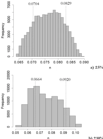
1000 depth values were generated, which varied between the measured depth value (Table 2) and ± 5% of this value, and another 1000 values
varying between the measured value and ± 10% of this value, being
this procedure done for the three stations. For example, for station
56425000, 1000 values were generated between 1.80 m and 1.98 m (‑5% and + 5% of 1.89 m, respectively) and 1000 values between 1.70 m and 2.08 m (‑10% and + 10% of 1.89 m, respectively).
For the generation of “Q” values, the same procedure
was used, that is, Uniform distribution was assumed and values
ranging from ± 5% to ± 10% in the measured “Q” value were
generated (Table 2). 1000 values of “Q” were generated for each
one of the generated “y” values. Thus, for each percentage of variation (5% and 10%), one million flow rates were generated (1000 flow rates times 1000 depths). This same amount of values
was generated for the three stations studied.
Each time a “y” was generated, 1000 values of “Q” were generated, and then a “n” was calculated for each one, that is, 1000 values of “n” were calculated for the generated “y”, and in
this calculation the regular cross section chosen for the station in question was used.
In the end, for each station, one million “n” were generated, via SMC, for the uncertainty of ± 5% and one million to ± 10%.
Then, for each station, the mean, maximum and minimum of these values were found, and it was observed how much they
deviated from the real “n”, which was calculated from the data of “Q” and “y” obtained in the field (Table 2). Using the deviations
of the found “n”, and their respective cross‑sections and “Q”
(Table 2), it was estimated how much these deviations can cause
variations of “y”.
RESULTS AND DISCUSSIONS
Determination of Manning’s roughness along the Doce River
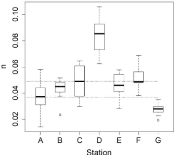
The values of “n” found for the seven Doce River river flow stations, which had bathymetry of their cross sections, are
presented in Figure 4. The medians of “n” of each season, in the order as presented in Figure 4, were: A) Fazenda Cachoeira
D’Antas (56425000) ‑ 0.037; B) Cachoeira dos Óculos (56539000) ‑ 0.045; C) Belo Oriente (56719998) ‑ 0.049; D) Governador Valadares (56850000) ‑ 0.085; E) Tumiritinga (56920000) ‑ 0.046; F) Resplendor (56948005) ‑ 0.049; G) Colatina (56994500) ‑ 0.028.
It is observed that the values of “n” undergo spatial
variation, since the medians are not equal among the stations,
with the median “n” of stations A, B, C, E, F being between
0.037 and 0.049 (dashed lines in Figure 4). On the other hand,
stations D and G, respectively, Governador Valadares and Colatina, are the ones that present more discrepant values.
This spatial variation of “n” was also observed by Zink and
Jennings (2014), who estimated values between 0.039 and 0.064 for five sections along a river in North Carolina, being those values
in the order of magnitude of those found by Matos et al. (2011), who estimated values ranging from approximately 0.030 to 0.070
for 36 sections along the Sapucaí River.
In the river flow station of Governador Valadares, the
median value of 0.085 was high, compared to the others. However,
it is in the same order of magnitude as that obtained by CPRM
(2004), which, for the definition of the floodplain of the city
homonymous to the station, based on hydraulic modeling made in HEC-RAS, allowed maximum values between 0.060 and 0.080 in all the cross sections used in the simulations. As the bottom of all cross sections of this station is very irregular, this may be
raising the value of “n”.
For Colatina, the median value of 0.028 was lower than the other stations, but it is close to that obtained by Coutinho (2015), who simulated flood spots in the city of Colatina using
HEC‑RAS, and defined Manning values for sections of the main
channel varying between 0.028 and 0.033. As this section of the Doce River is very silted, with the roughness of the sand in the
order of 0.016, this may have caused a decrease in the value of “n”.
Both the work of CPRM (2004) and Coutinho (2015)
used HEC‑RAS to calibrate the values of “n”, being in the same
order of magnitude as those obtained in this article. It is observed, then, that the methodology used in this study presented results
compatible with the studies that used HEC‑RAS to calibrate “n”. Figure 4 shows that, for the same river flow station, the variation of “n” occurs over time, which was also observed by
Lyra et al. (2010) for the Paracatu River, and these authors showed
that the roughness coefficients varied significantly among the
seasons. Some stations, such as Belo Oriente (C), presented large deviations from the values, whereas in Colatina (G) all values found are close to the median. Thus, in a hydraulic modeling over a long period of time, care must be taken when adopting a single Manning for the entire modeling period.
Relation between water depth and Manning coefficient
Table 3 shows the p-value found when applying the
Shapiro‑Wilk test for the seven stations. It has been shown that all p‑values were higher than 0.05 (level of significance), both for the
Figure 4. Spatio-temporal variation of Manning’s roughness
case where Manning (ndaily) was found using daily data of “y” and
“Q”, as for the case where we worked with monthly mean values of “y” and “Q” to calculate Manning (nmonthly). Thus, the two sets with
values of “n” follow Normal distribution, following the premise for the use of Student’s t‑test. For example, for station 56425000 a
p-value of 0.52 (ndaily) was obtained for the set of Manning values
found using daily data of “y” and “Q” and 0.44 (nmonthly) for the
set obtained from monthly mean values of “y” and “Q”. As these values are greater than the level of significance, it is known that these roughness coefficients are normally distributed.
Also in Table 3, there is no significant difference between the
“n” values found by the two procedures used (“ndaily” e “nmonthly”),
since all p-values found in the application of Student’s t-test
were greater than 0.05. For example, for station 56425000, the “n” values found by the two procedures were 0.0421 and 0.0427,
and since the p-value was 0.16 (Table 3), statistically there was no difference between them.
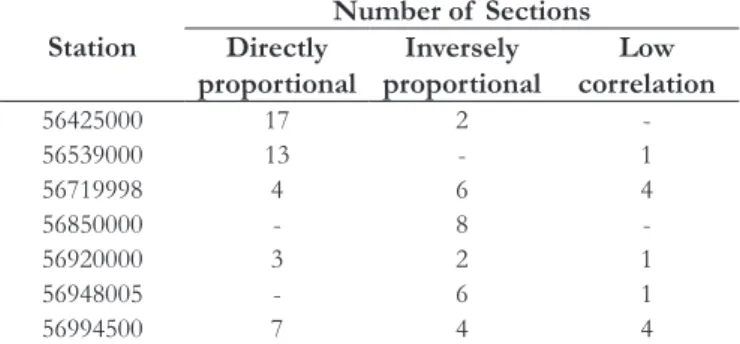
Table 4 shows the behavior of the variation of “n” (for each station) due to the variation of “y” along the hydrological year of each cross section. For example, for station 56425000, of the 19 cross‑sections analyzed, it is found that by varying “y” and calculating “n”, in 17 profiles the relation between these
variables was directly proportional, while in two it was inversely proportional . It can be observed that for most stations there is not only one behavior, that is, in some sections the relation between these variables was directly proportional throughout the year, corroborating with Lyra et al. (2010), while in others it was inversely proportional, as observed by Zink and Jennings
(2014), Fathi and Drikvandi (2012), Matos et al. (2011), Kim et al.
(2010) and Chow (1959). There were also sections where it was not possible to observe any correlation between the two variables.
One explanation for not having a single rule for the relation between these two variables is the cross section format and the
range of “y” in this section. Observing the relation between these
variables, for each cross section of each station, it was noticed
that when the section tends to have two defined beds, one bigger
and one smaller, the relation between the variables tends to be
directly proportional when the flow occurs in the higher bed and inversely proportional when the flow is at the lowest, as expected. This happens because the larger bed may be the floodplain, where
there are several materials, such as vegetation, gravel, among others, which increases the value of Manning (PARSAIE et al., 2017).
While in the lower bed, where consequently the flow has a lower
depth, the effects of canal bottom irregularities are more evident, which increases Manning’s value (CHOW, 1959).
An example that illustrates the previous assertion is in Figure 2, where it is presented in (a) the cross section of the
year 2014 of the river flow station Fazenda Cachoeira D’Antas
(56425000). In Figure 2b is the curve representing the variation
between “n” and “y” along the hydrological year of 2014 and also
the regression equation of this curve is presented. It is observed in Figure 2a that for depths smaller than approximately 2.00 m
the flow is in the smaller channel of the river. In Figure 2b, it is
observed that for “y” up to approximately 2.20 m, the variation of “n” is inversely proportional to “y”, while for “y” the relation
becomes directly proportional. In general, in other stations the behavior was the same occurred in Fazenda Cachoeira D’Antas.
Observing Table 4, it can be noted that only in the
Governador Valadares (56850000) and Resplendor (56948005) stations the relation between “n” and “y” was always inversely
proportional, and the possible reason for this to happen is the fact that all the cross sections of these stations do not clearly show the existence of two beds, as observed in Figure 2a.
For each station, when all the annual mean values of
“n” and their respective annual “y” values were plotted, it was
observed that in none of them there was correlation between these variables over the years. Figure 3 shows the behavior between
these variables for Fazenda Cachoeira D’Antas station (56425000),
which represents the other stations, since the behavior is the same, and the number of points in the graph indicates the number of cross sections that existed for the station, that is, each point is an
annual average “n” and “y” value of a section.
It is noticed that there is no possibility of only one equation
to relate these variables, since it cannot explain the behavior of “n” over the years. One reason for such a random behavior between “n” and “y” is the fact that the constant change of the cross‑sections,
as shown in Figure 5, in which is presented the change occurred
in the cross section between the years of 2013 and 2014, in the station Fazenda Cachoeira D’Antas (56425000). It is noteworthy
that this change in the cross sections occurred for the seven river
flow stations studied. Thus, the roughness of a given year has no
correlation with that of a subsequent year and/or later.
In order to confirm the lack of autocorrelation between
the values of “n” over the years, the correlogram (Figure 6) was
constructed for the roughness of Fazenda Cachoeira D’Antas, which was presented in Figure 3. In this correlogram, it is noted
that there is no significant autocorrelation (ACF) for any Lag, since they are all within the limits of confidence (dashed lines).
Table 4. Relation between the variation of Manning coefficient
and water depth.
Station Directly Number of Sections
proportional proportionalInversely correlationLow
56425000 17 2
-56539000 13 - 1
56719998 4 6 4
56850000 - 8
-56920000 3 2 1
56948005 - 6 1
56994500 7 4 4
Table 3. p-values for the applied statistical tests.
Station
Shapiro-Wilk Student’s
T-test p-value
p-value
ndaily nmonthly
56425000 0.52 0.44 0.16
56539000 0.69 0.73 0.18
56719998 0.36 0.45 0.30
56850000 0.86 0.88 0.18
56920000 0.52 0.44 0.17
56948005 0.71 0.69 0.35
Uncertainties associated with Manning coefficient values
Figures 7 to 9 show the values of “n” generated from the Monte Carlo Simulation (SMC). The dashed lines indicate the
quartiles of probability, being the 25% quartile the first line and the 75% quartile the second. Although the values of flows and depths, which originated the values of “n”, follow the Uniform distribution, it can be seen from the figures that “n” does not
tend to follow the same probability distribution.
Table 5 shows the uncertainties associated with the
values of “n” due to errors of ± 5 and ± 10% in the flow rate measurement (Qreal) and depth (yreal). Considering as the correct Manning (nreal) the one calculated from the data measured in the
field, which are recorded in the historical series of the stations, it is observed that an error of ± 5% causes the greatest uncertainty,
Figure 5. Alteration of the cross section of Fazenda Cachoeira
D’Antas between the years of 2013 and 2014.
Figure 6. Correlogram for the average annual roughness of
Fazenda Cachoeira D’Antas.
Figure 7. Manning’s Roughness coefficient via SMC for Fazenda
Cachoeira D’Antas.
Figure 8. Manning’s Roughness coefficient via SMC for Governador
of 1.72%, in the value of the average “n” of Fazenda Cachoeira D’Antas station (56425000) and the lowest uncertainty of 0.99% for Governador Valadares (56850000). For an error of ± 10%, the highest uncertainty for the mean “n” is 1.72% for Colatina (56994500) and the lowest, of 1.01%, for Governador Valadares
(56850000).
Figure 9. Manning’s Roughness coefficient via SMC for Colatina
station (56994500).
Table 5. Uncertainties associated to the values of the Manning coefficient due to errors of ± 5 and ± 10% in the flow values of
depths measured in the field.
Station Qreal
(m3/s) yreal (m)
Error (%)
n
nreal Uncertainties of n (%)
Max Average Min Max Average Min
(56425000) 37.15 1.89 5 0.0748 0.0589 0.0444 0.0579 29.21 1.72 23.23
10 0.0927 0.0590 0.0312 60.06 1.38 46.05
(56850000) 418.7 3.33 5 0.0891 0.0764 0.0642 0.0757 17.65 0.99 15.19
10 0.1047 0.0749 0.0537 38.30 1.01 29.04
(56994500) 446.8 2.45 5 0.0349 0.0275 0.0217 0.0279 25.28 1.29 21.99
10 0.0432 0.0283 0.0166 54.75 1.72 40.52
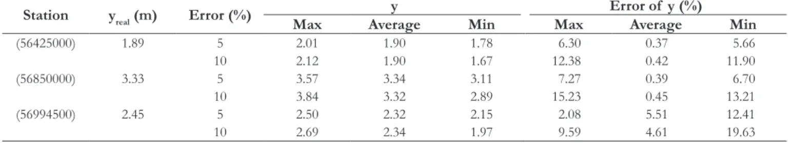
Table 6. Uncertainties associated to the simulated depths with the values of “n” obtained via SMC.
Station yreal (m) Error (%) y Error of y (%)
Max Average Min Max Average Min
(56425000) 1.89 5 2.01 1.90 1.78 6.30 0.37 5.66
10 2.12 1.90 1.67 12.38 0.42 11.90
(56850000) 3.33 5 3.57 3.34 3.11 7.27 0.39 6.70
10 3.84 3.32 2.89 15.23 0.45 13.21
(56994500) 2.45 5 2.50 2.32 2.15 2.08 5.51 12.41
10 2.69 2.34 1.97 9.59 4.61 19.63
When comparing the “nreal” with the maximum “n” values
obtained, for ± 5% of variation, it is noticed that the greatest
uncertainty occurs in the Fazenda Cachoeira D’Antas station
(56425000), where the maximum value found (0.0748) deviates from the real value (0.0579) in 29.21%. For ± 10% variation, the
highest uncertainty occurs at the same station, where the difference between the maximum value (0.0927) and the real value (0.0579)
was 60.06%.
In the case of comparing the “nreal” with the minimum
“n” values, for ± 5% of variation, the greatest uncertainty was obtained for Fazenda Cachoeira D’Antas station (56425000), since the difference between the minimum value found (0.0444) and the real value (0.0579) was 23.23%. For ± 10%, again the greatest uncertainty, which was 46.05%, occurred at Fazenda Cachoeira D’Antas station (56425000).
Thereby, it can be seen that the greatest uncertainties, both for the maximum and the minimum, were for the station with the
lowest flow rate and depth, corresponding to Fazenda Cachoeira D’Antas, showing that errors in low values of “Q” and “y” may cause greater uncertainties in the “n” values.
Table 6 shows the values of “y” obtained from the Manning
coefficients generated by SMC (maximum, average and minimum
presented in Table 5). It is also shown how much these “y”
distanced themselves from the depth (yreal) measured in the field. For ± 5 and ± 10%, using the average “n” value generated
by SMC to simulate the values of “y”, in Table 6, it is noticed
that the largest error in the calculated “y” was for the station of Colatina (56994500), when the variation was ± 5%, and this error was 5.51%. The lowest error was 0.37% for a variation of ± 5%
in Fazenda Cachoeira D’Antas station (56425000). Kim et al.
(2010) found maximum error of 4.2% in the value of “y”, for
10% of variation, and minimum of 2.3%, for 5% of variation.
Thus, it is observed that even if there are uncertainties in the
mean “n” values, the impact caused by the “y” value was small
stations studied, so that the variation of “y” is small, and in case of narrow channels the uncertainty in the value of “n” may cause greater variation in the simulated “y” value.
When the extreme values of “n” (maximum and minimum
of Table 5) were used to calculate “y”, it was obtained that the
simulated depths were more distant from the real ones. When using the maximum “n” from Table 6, it is noticed that the largest
error in the simulated “y” value was 15.23% in the Governador Valadares station (56850000), for a variation of ± 10%, being this error the difference between the simulated depth, 3.84 m, and the actual depth, 3.33 m. In regarding to the minimum “n”,
the simulated depth of 1.97 m was the most distant from the real
one, 2.45 m, a fact observed in the Colatina station (56994500), being this error of 19.63% obtained for the variation of ± 10%. It is observed, then, that the extreme “n” caused a maximum
variation of ± 0.5 m in the water depth. Again, it is emphasized that in narrow channels the variation in water depth may be greater.
CONCLUSION
Manning’s roughness coefficients were estimated for seven river flow stations installed along the Doce River. From these
values, we have that:
• The Manning coefficient values undergo spatial‑temporal
variation along the Doce River, and the median values
for the stations Fazenda Cachoeira D’Antas (56425000),
Cachoeira dos Óculos (56539000), Belo Oriente (56719998),
Tumiritinga (56920000) and Resplendor (56948005) are
within the same range of values. On the other hand, the stations Governador Valadares (56850000) and Colatina
(56994500) present median values that differ from the others. However, it should be noted that the median values of “n”
of the stations may not represent the period of maximum
river flow rates, since, as presented in the methodology, in no station there was a determined cross section profile
in the rainy season, so that the Manning values that were
found are all referring to the flow rates between April and
November. Because the Manning values undergo temporal variation, it is suggested that hydraulic models, for the Doce River, can be made separated by shorter periods of time,
so that each period uses a different Manning coefficient.
• There is not a single relation between Manning’s values and water depth, which means that there are cases in which this relation is directly and other cases in which it is inversely proportional, for the same station. This is due to the shape of the cross section, being that when there are two beds, a bigger and a smaller one, the tendency is that the relation between these variables is inversely proportional in the smaller bed and directly proportional in the larger one. Thus, for the Doce River, attention should be paid when using some equation from literature that relates exclusively
water depth to the Manning coefficient, since this relation
is variable in time.
• The historical series of flow rates and water levels were
known, however, this does not mean that there are not inaccuracies in their values. As these series were used for
determining the roughness, inaccuracies in the “n” values
could consequently occur. Thus, these uncertainties were analyzed. For this, three river stations were studied, one for each region of the Doce River, and it was obtained that
errors of ± 5 and ± 10% in the value of the flow rate and of
water depth originated low percentages of uncertainties in the average values of Manning. However, there were extreme point values (maximums and minimums) that distanced
themselves more from the real value of Manning. When using the average values of “n” to simulate depth values, the simulated “y” values were close to those measured in the field, ie, this average value of “n” had little effect on the final result of the waterline simulations. However,
this conclusion can not be extended to all hydrodynamic models, since only one model was evaluated in this work (Canal software), which uses the Manning Equation to
simulate flow depths. When “y” was simulated using extreme “n” values, a greater variation was obtained between the simulated and the real “y”, with a maximum
variation of ± 0.5 m. However, it is noteworthy that the cross sections of the three stations were broad, and in narrower sections, which have greater water depth variation, the uncertainties in the Manning values may cause greater variation in the simulated depths.
Recently, the Doce River was highlighted because of everything that involved the dam collapse in Mariana (the position of this city in the Doce River basin is presented in Figure 1), which culminated in a large volume of tailings thrown into the
river. Because of this, in some places the roughness coefficient
may have been affected, since the mining tailings, which have a
specific weight greater than that of water, deposited at many points,
changing the material and shape of the cross-section. However, the cross sections topographies of immediately after the tailings
passage were not available, so that, in this work, the influence of
these tailings in the value of Manning was not analyzed. Thus, it is recommended to continue this study in order to evaluate the
probable changes in the Manning coefficients due to the dam
rupture in Mariana.
In the analysis of uncertainties, the influence of inaccuracies in the slope of the sections in the value of the roughness coefficient
was not evaluated, so that this should be done in future works, in
order to continue the verification of the behavior of the Manning coefficient of the Doce River.
ACKNOWLEDGEMENTS
To the Federal University of São João del‑Rei for financial
support and the postgraduate program in Sanitation, Environment
and Water Resources of the Federal University of Minas Gerais.
REFERENCES
CALO, V. M.; COLLIER, N.; GEHRE, M.; JIN, B.; RADWAN,
H.; SANTILLANA, M. Gradient-based estimation of Manning’s friction coefficient from noisy data. Journal of Computational and Applied Mathematics, v. 238, p. 1-13, 2013. http://dx.doi.org/10.1016/j.
cam.2012.08.004.
CBH-DOCE – COMITÊ DA BACIA HIDROGRÁFICA DO RIO DOCE. Diagnóstico consolidado da bacia do Rio Doce. Governador Valadares: CBH-DOCE, 2005.
CBH-DOCE – COMITÊ DA BACIA HIDROGRÁFICA DO RIO DOCE. Plano Integrado de Recursos Hídricos da Bacia do Rio Doce (PIRH). Governador Valadares: CBH-DOCE, 2013.
CHOW, V. T. Open channel hydraulics. New York: McGraw-Hill, 1959.
COUTINHO, M. M. Avaliação do desempenho da modelagem hidráulica unidimensional e bidimensional na simulação de eventos de inundação em Colatina/ES. 2015. 245 f. Dissertação (Mestrado em Saneamento,
Meio Ambiente e Recursos Hídricos) – Escola de Engenharia,
Universidade Federal de Minas Gerais, Belo Horizonte, 2015.
CPRM – SERVIÇO GEOLÓGICO DO BRASIL. Definição da planície de inundação da cidade de Governador Valadares: relatório técnico
final. Belo Horizonte: CPRM, 2004. p. 128.
FARD, R. S.; HEIDARNEJAD, M.; ZOHRABI, N. Study factors
influencing the hydraulic roughness coefficient of the Karun river (Iran). International Journal of Farming and Allied Sciences, v. 22, n. 2, p. 976-981, 2013.
FATHI, M. M.; DRIKVANDI, K. Manning roughness coefficient for rivers and flood plains with non-submerged vegetation. International Journal of Hydraulic Engineering, v. 1, n. 1, p. 1‑4, 2012.
GOLSHAN, M.; JAHANSHAHI, A.; AFZALI, A. Flood hazard zoning using HEC-RAS in GIS environment and impact of manning roughness coefficient changes on flood zones in Semi-arid climate. Desert, v. 21, n. 1, p. 24‑34, 2016.
KIM, J. S.; LEE, C. J.; KIM, W.; KIM, Y. J. Roughness coefficient and its uncertainty in gravel-bed river. Water Science and Engineering, v. 3, n. 2, p. 217-232, 2010.
KIM, W.; KIM, Y. S.; WOO, H. S. Estimation of channel roughness coefficients in the Han river using unsteady flow model. Hangug Sujaweon Haghoe Nonmunjib, v. 28, n. 6, p. 133‑146, 1995.
KIM, Y.; TACHIKAWA, Y.; SHIIBA, M.; KIM, S.; YOROZU,
K.; NOH, S. J. Simultaneous estimation of inflow and channel roughness using 2D hydraulic model and particle filters. Journal of Flood Risk Management, v. 6, n. 2, p. 112-123, 2013. http://dx.doi.
org/10.1111/j.1753‑318X.2012.01164.x.
KOPECKI, I.; SCHNEIDER, M.; TUHTAN, J. A. Depth-dependent hydraulic roughness and its impact on the assessment
of hydropeaking. The Science of the Total Environment, v. 575, n. 1, p. 1597-1605, 2017. http://dx.doi.org/10.1016/j.scitotenv.2016.10.110. PMid:27802885.
LYRA, G. B.; CECÍLIO, R. A.; ZANETTI, S. S.; LYRA, G. B.
Coeficiente de rugosidade de Manning para o Rio Paracatu. Revista Brasileira de Engenharia Agrícola e Ambiental, v. 14, n. 4, p. 343‑350, 2010. http://dx.doi.org/10.1590/S1415‑43662010000400001.
MATOS, A. J. S.; PIOLTINE, A.; MAUAD, F. F.; BARBOSA, A. A. Metodologia para a caracterização do coeficiente de Manning variando na seção transversal e ao longo do canal. Estudo de caso
bacia do Alto Sapucaí‑MG. RBRH: Revista Brasileira de Recursos
Hídricos, v. 16, n. 4, p. 21‑28, 2011. http://dx.doi.org/10.21168/
rbrh.v16n4.p21‑28.
MTAMBA, J.; VAN DER VELDE, R.; NDOMBA, P.; ZOLTÁN,
V.; MTALO, F. Use of Radarsat-2 and Landsat tm images for spatial parameterization of Manning’s roughness coefficient in hydraulic modeling. Remote Sensing, v. 7, n. 1, p. 836‑864, 2015. http://dx.doi.org/10.3390/rs70100836.
NIMNIM, H. T.; FARHAN, B. A. Evaluation of Manning’s coefficient of ferrocement trapezoidal and semicircle canals strengthened by CFRP sheets. International Journal of Energy and Environment, v. 6, n. 5, p. 461‑470, 2015.
PARHI, P. K.; SANKHUA, R. N.; ROY, G. P. Calibration of channel roughness for Mahanadi River (India), using HEC-RAS model. Journal of Water Resource and Protection, v. 4, n. 10, p. 847‑850, 2012. http://dx.doi.org/10.4236/jwarp.2012.410098.
PARSAIE, A.; NAJAFIAN, S.; OMID, M. H.; YONESI, H. Stage discharge prediction in heterogeneous compound open channel roughness. Journal of Hydraulic Engineering, v. 23, n. 1, p. 49‑56, 2017.
http://dx.doi.org/10.1080/09715010.2016.1235471.
PRAJAPATI, P. R.; VADHER, B. M.; YADAV, S. M. Comparative analysis of hydraulic roughness coefficient at Purna River sites. Global Research and Development Journal for Engineering, v. 1, n. 4, p.
574‑579, 2016.
PRUSKI, F. F.; SILVA, D. D.; TEIXEIRA, A.; CECÍLIO, R. A.; SILVA, J. M. A.; GRIEBELER, N. P. Hidros: dimensionamento
de sistema hidroagrícolas. Viçosa: Editora UFV, 2006. 259 p.
UFV – UNIVERSIDADE FEDERAL DE VIÇOSA. Grupo
de Pesquisa em Recursos Hídricos. Softwares. Viçosa: UFV, 2018.
Disponível em: <http://www.gprh.ufv.br/?area=softwares>.
Acesso em: 31 jan. 2018.
ZINK, J. M.; JENNINGS, G. D. Channel roughness in North
Authors contributions
Emmanuel Kennedy da Costa Teixeira: Work creator. Executor
of all work steps and article text writer.
Márcia Maria Lara Pinto Coelho: PhD advisor of the first author
of this paper. Guiding all stages of the work. Revision of the text of the article.
Eber José de Andrade Pinto: Guiding all stages of the work.
Reviewer of the text of the article.
Jéssica Guimarães Diniz: Executing the work. He effectively
participated in the tabulation of the thousands of data, as well as the simulations of the data made in the hydraulic program.