P
UBLIC DEBT AND THE LIMITS OF FISCAL POLICY TO
INCREASE ECONOMIC GROWTH
VLADIMIR KUHL TELES
CAIO CESAR MUSSOLINI
Novembro
de 2011
T
T
e
e
x
x
t
t
o
o
s
s
p
p
a
a
r
r
a
a
D
D
i
i
s
s
c
c
u
u
s
s
s
s
ã
ã
o
o
TEXTO PARA DISCUSSÃO 304•NOVEMBRO DE 2011• 1
Os artigos dos Textos para Discussão da Escola de Economia de São Paulo da Fundação Getulio Vargas são de inteira responsabilidade dos autores e não refletem necessariamente a opinião da
FGV-EESP. É permitida a reprodução total ou parcial dos artigos, desde que creditada a fonte.
Escola de Economia de São Paulo da Fundação Getulio Vargas FGV-EESP
Public Debt and the Limits of Fiscal Policy to Increase
Economic Growth
Vladimir K¨uhl Teles
∗Caio Cesar Mussolini
†October 27, 2011
Abstract
Research that seeks to estimate the effects of fiscal policies on economic growth has ignored the role of public debt in this relationship. This study proposes a theoretical model of endogenous growth, which demonstrates that the level of the public debt-to-gross domestic product (GDP) ratio should negatively impact the effect of fiscal policy on growth. This occurs because government indebtedness extracts part of the savings of the young to pay interest on the debts of the older generation, who are no longer saving. Therefore, the payment of debt interest assumes an allocation exchange role between generations that is similar to a pay-as-you-go pension system, which results in changes in the savings rate of the economy. The major conclusions of the theoretical model were tested using an econometric model to provide evidence for the validity of this conclusion. Our empirical analysis controls for time-invariant, country-specific heterogeneity in the growth rates. We also address endogeneity issues and allow for heterogeneity across countries in the model parameters and for cross-sectional dependence.
Key Words:Public Debt, Endogenous Growth, Fiscal Policy
JELs:O23, O41, O54.
1
Introduction
This article examines how the size of the public debt-to-GDP ratio limits the effects of productive
govern-ment expenditures on long-term growth. We conducted this analysis by proposing a model with
overlap-ping generations and endogenous growth, wherein the government can go into debt in order to increase
its productive expenditures. Various works present models where public expenditures affect growth via a
framework of endogenous growth (Barro, 1990; Chen, 2006; Devarajan et al., 1996; Glomm and
Raviku-mar, 1997), wherein the effect of these expenditures varies according to their nature, their composition,
and the size of the tax burden. Other works demonstrate that public debt can negatively affect growth
(Brauninger, 2005; Saint-Paul, 1992). In this article, we establish a link between these two classes of
models and demonstrate that the effect of productive expenditures on growth is limited not only by the
size of the tax burden and the rate of indebtedness, as predicted by these models, but also by the
debt-to-GDP ratio.
Similar to the models of Barro (1990) and Saint-Paul (1992), the model that we propose here
demon-strates that an increase in public expenditures can have three direct effects on growth. An increase in
public expenditure positively affects economic productivity but at the expense of the negative effects that
are associated with the increases in the tax burden and public indebtedness in order to finance the
expen-ditures, which result in a decrease in savings; however, in our approach, we demonstrate that there is an
additional indirect effect: an increase in productive expenditures results in an increase in the equilibrium
interest rate due to the increase in productivity. This results in an increase in expenditures for interest
rate on public debt and an additional reduction in savings. This occurs because government indebtedness
extracts part of the savings of the young to pay interest on the debts of the older generation, who are
no longer saving. Therefore, the payment of debt interest assumes an allocation exchange role between
generations that is similar to a pay-as-you-go pension system, which results in changes in the savings rate
of the economy.
In the second part of the article, we will estimate a growth equation using the specification proposed
by the theoretical model for a panel of countries to provide valid evidence for the conclusions of the
theoretical model. Our empirical analysis controls for time-invariant, country-specific heterogeneity in
the growth rates. We also address endogeneity issues and allow for heterogeneity across countries in the
model parameters and for cross-sectional dependence.
Various studies have found empirical evidence that the allocation of public funds towards education,
health, and infrastructure expenses positively impact economic growth (Aschauer, 1989; Easterly and
Rebelo, 1993; Gupta et al., 2005); however, there is no consensus regarding this issue, as many works find
insignificant results (Agell et al., 2006; Devarajan et al., 1996). We suggest that the disagreement among
these works can be reconciled by taking a closer look at the theory. We used a specified theoretical model
that clarifies the proper non-linear specification of our growth regression and allows us to demonstrate
that by disregarding the role of public debt in this relationship, the estimations that are used in previous
studies can result in omitted variable bias. In addition, we find evidence that the magnitude of the effect
2
Theoretical Model
In this section, a simple overlapping generations model of endogenous economic growth will be
devel-oped, wherein it is established that public expenditures can affect economic productivity. The model is
an extension of Barro (1990) and Glomm and Ravikumar (1997) in that the government can become
indebted in order to increase its productive expenditures.
2.1
Agents
If an overlapping generations model in which each generation lives for two periods and consists of a
continuum of identical individuals in the interval(0,1)is considered, the utility function of an agent who
is born in the periodt= 0,1, ...is defined by:
U =lnct
t+βlnc t
t+1 (1)
wherect
i is consumption in the periodiof the individual who is born intand0< β <1. The initial
gen-eration of older people is endowed withk0 units of capital. The following generations are each endowed
with one unit of labor. The youth from generationthave the following restrictions:
ct
t+stt ≤(1−τ)wt, (2)
ct
t+1≤(1 +rt+1)stt, (3)
(ctt, c t
t+1)≥0, (4)
wherest
t = kt+1+dt+1 is savings and dtare government bonds that are owned by private agents. Each
individual takes the wage rate,wt, the real interest rate, rt+1, and the tax rate, τ, as given. Clearly, one
unit of labor is inelastically supplied by each young individual and no old individual wishes to save.
2.2
Firms
There is a representative firm that attempts to maximize its profits in an environment of perfect
competi-tion, and it has the following production function:
yt=Az
1−α t k
α
t (5)
whereytis the output,ztare the productive government expenditures, that is, the expenditures that affect
the marginal product of capital, andktis the capital stock that is rented by the firm following the law of
accumulationkt+1 = (1−δ)kt+it, whereδis the depreciation rate anditis the level of investment. For
simplicity, let us assumeδ= 1. This production function is identical to Barro’s (1990) if we assume that
the quantity of productive expenditures as a part of the aggregate product.
zt=xyt (6)
wherexis the fraction of production that is designated for productive expenditures. Using (6) in (5), we
now have
yt =A
1 αx1−
α
α kt (7)
Therefore, the economy’s production function exhibits constant marginal returns for capital, despite
the fact that the returns for firms are decreasing. This is a result of the externality of productive
gov-ernment expenditures. The firm does not perceive that by increasing capital stock (and consequently the
product), there will be an increase in productive spending by the government, and this leads to an increase
in the marginal products of labor and capital.
2.3
Government
The government spends a fixed fraction0 < g < 1of the product on its consumption and also spends a
fractionxand charges a tax rateτ on the income of the agents. In addition, it borrows resources from the
private sector by issuing bondsdtthat pay a remuneration ofrt+1 in the following period, whered0 = 0.
Therefore, changes in government debt are expressed as the primary deficit(g+x)yt−τ wtadded to the
debt service paymentsrtdt.
dt+1−dt=rtdt+ (g+x)yt−τ wt (8)
In order for the government to meet its budgetary restrictions, we have to assume that some component
of the government budget is endogenous, serving as an adjusted variable. Thus, we will assume that the
government always adjusts its indebtedness to satisfy its budgetary restriction. This is relevant because
we are assuming that each time that the government decides to increase its expenditures, it also decides
to increase its indebtedness. For the case of study in this manuscript, specifically, productive government
expenditures, we observe that governments increase the product by raising productivity; however, their
increase results in a larger deficit, such that productive expenditures have a limited effect on the economy
because they are financed by increases in the public debt.
2.4
Competitive Equilibrium
Givenk0, a competitive equilibrium for this economy involves a sequence of allocations{kt+1, dt+1, yt,
ct
t,ctt+1,s
t t}
∞
t=0and prices{wt, rt} ∞
t=0, such that:
1. Given wt and rt+1, the allocation (ctt, ctt+1, stt) resolves the maximization problem for the young
2. Given wt and rt, the allocation (yt, kt) resolves the maximization problem for the representative
firm,
3. st
t=kt+1+dt+1,
4. yt=ctt+c t−1
t +kt+1+gyt+xyt.
The solution to the optimization problem for the younger generation in periodtyields:
st
t =β(1−τ)wt/(1 +β) (9)
The profit maximization of the firms leads to:
∂yt
∂kt
=αAz1−α t k
α−1 t =rt
Substituting (6) and (7) into this equation, we find
rt=αA
1
αx1−αα (10)
and, given that the technology exhibits constant returns to scale with the private factors, economic profit
does not exist; therefore,
yt−
∂yt
∂kt
kt = (1−α)Az
1−α t kα
−1 t =wt
and analogously
wt = (1−α)A
1 αx1−
α
α kt (11)
Therefore, because productive government expenditures affect the productivity of the economy, they
naturally also affect interest rates and wages. Since the present model is represented in the AK form,
savings affect long-term growth. Equation (9) demonstrates that shocks to the equilibrium wage lead to
greater savings, and equation (11) makes it clear that shocks to productive government expenditures(11)
increase the wage level. Therefore, increases in productive expenditures lead to permanent productivity
shocks and salary increases. This produces an increase in savings, investments, and subsequently, in
economic growth.
However, it is important to note that in (9), the savings increase depends negatively on τ, as this
decreases the net gain of the productivity increase. This result is consistent with that obtained by Barro
(1990), in that increases in productive expenditures depend in a non-linear way on the size of government.
Using (7), (8), (10), and (11) in equation (9) and a bit of algebra, the capital growth rate is given by:
kt+1−kt
kt
=−1+ β
1 +β(1−τ)(1−α)A 1 αx1
−α
α −[g+x−(1−α)τ]Aα1x1 −α
α −(1+αAα1x1 −α
α )dt kt
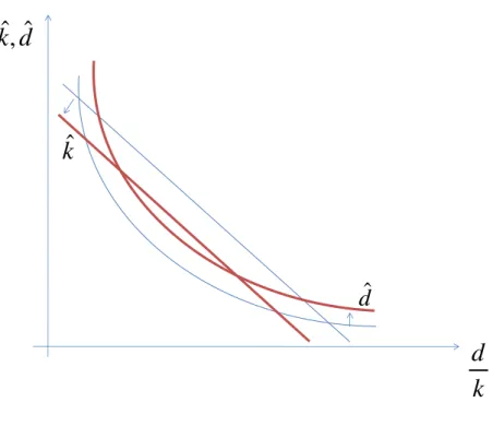
Figure 1:
k
ˆ
d
ˆ
k
d
d
k
ˆ
,
ˆ
Initially, we will assume that there is a stable equilibrium in the economy or that dt
kt is constant. In
this case, equation (12) demonstrates the dynamic equilibrium of capital and, consequently, that of the
product. There are three components in the right-hand side of the equation that show us the three paths
by which an increase in productive government expenditures can affect growth.
The first part of the equation demonstrates that an increase in productive expenditures increases
growth, which reflects their impact on the economy’s productivity by increasing aggregate savings and
economic growth; however, once again, the size of this effect decreases as the size of the tax burden
increases.
The second component of the equation will be zero if the primary deficit in relation to the GDP
[g +x−(1−α)τ] is zero. This component also shows that the marginal effect of productive govern-ment expenditures varies depending on the primary deficit. This demonstrates that when the governgovern-ment
increases its productive expenditures, such as in education, infrastructure, or health, there is a negative
effect on growth because it directly increases government indebtedness and reduces the savings that is
designated for private investment.
The third component of the equation reproduces the indirect impact that productive government
ex-penditures have on indebtedness and, therefore, on growth. Because increases inxraise the interest rate
and because the government pays interest rate on public debt, an increase in productive expenditures
impacts the costs of the debt, which indirectly raises the rate of government indebtedness. Thus, as the
public debt increases in size, this relationship becomes more perverse such that productive expenditures
Figure 2: Increase in Government Consumption (g)
d
k
ˆ
,
ˆ
k
ˆ
d
ˆ
k
d
Figure 3: Increase in Productive Expenditures (x)
ˆ ˆ
,
k d
d
k
ˆ
k
ˆ
Models with budgetary equilibrium, as found in Barro (1990); Glomm and Ravikumar (1997), only
provide results for the first part of the equation. The second component of the equation follows the same
logic as the models of debt and endogenous growth that are found in Saint-Paul (1992), wherein increases
in the public debt lead to greater indebtedness, which decreases the amount of savings that is allocated to
capital accumulation. In our approach, we find an additional effect (the third part of the equation) where
the size of the debt becomes relevant. We can understand this effect as being similar to a pay-as-you-go
pension system, in that a portion of the savings of the young is reallocated to pay the older generation
(through greater debt interest payments) instead of on the accumulation of capital, thereby diminishing
economic growth.
Thus, the magnitude of the impact of an increase in productive expenditures on economic growth
varies based on the size of the primary deficit and the public debt. In other words, it is more likely that
increases in infrastructure, education, and health expenditures, or any other productive expenditures, will
stimulate economic growth when the unproductive portion of the government and the debt-to-GDP ratio
are lower.
In order to verify and characterize whether there is asteady-stateequilibrium in the economy, we have
to examine the debt dynamics. Thus, by substituting (7),(10) and (11) in (8) and dividing bydt, we have:
dt+1−dt
dt
=αAα1x1 −α
α + [g+x−(1−α)τ]Aα1x1 −α α kt
dt
(13)
Thus, for the growth rates ofkt and dt to be constant, or rather, so that there is an equilibrium, the
ratiodt/ktneeds to be constant, such thatkt+1/kt=dt+1/dt. By setting equations (12) and (13) equal to
one another, we obtain a quadratic equation for the equilibrium debt-capital ratio, the solution to which is
defined by:
d
k =
n
β
1+β(1−τ)(1−α)−α−[g+x−(1−α)τ]
o
Aα1x1− α
α −1±√H
2[1 +αAα1x1− α α ]
H ≡ {[ β
1 +β(1−τ)(1−α)−α−[g+x−(1−α)τ]]A 1 αx1
−α α −1}2
−4(1 +αAα1x1 −α
α )) [g+x−(1−α)τ]Aα1x1 −α
α
Thus, if the solution above possesses at least one real positive root, there is asteady-stateequilibrium.
Naturally, the existence of an equilibrium depends on the values of the model parameters, and as
demon-strated exhaustively by Brauninger (2005), an equilibrium is not always obtained for plausible parameter
values.
In Figure 1, where ˆkanddˆare the capital and debt growth rates, equations (12) and (13) are plotted
in an example where we assume that the two roots are real and positive and[g+x−(1−α)τ]>0. In Figure 1, we have a result with two equilibriums: the first, which is characterized by a low
debt-capital ratio, a low debt-GDP ratio, and high economic growth, is locally stable, whereas the second,
In Figure 2, we evaluate a scenario in which an economy in equilibrium experiences an increase in
unproductive government expenditures (g). In this case, the capital growth curve shifts downwards and
the debt growth curve shifts upwards. If the economy is initially in a state of stable equilibrium with high
growth, this leads to a decline insteady-stateeconomic growth and an increase in the debt-to-GDP ratio.
In an extreme situation with an excessive increase in unproductive expenditures, the two curves no longer
intersect, meaning that the growth rate of debt would be larger than that of the economy and suggesting an
explosive increase in debt and an absolute collapse of the economy. This would be the case if there were
nosteady-stateequilibrium. This result is essentially the same as that obtained by Brauninger (2005).
However, the case that most interests us, and for which this article attempts to make a contribution,
is that of increases in productive government expenditures. This case is illustrated in Figure 3. With an
increase in productive expenditures (x), the slopes of the two curves change. In this example, where the
economy is in a stable steady-state, economic growth increases, as does the debt-to-GDP ratio. This
occurs because the fiscal cost of increasing this type of spending is still small in comparison to the
resulting productivity gains. Consequently, the economy still has the necessary fiscal strength, and this
type of policy is very successful; however, at an equilibrium with a high debt-to-GDP ratio, the effect
on growth and the increase in productive expenditures will be less substantial, and the effect on the
debt-capital ratio is uncertain because it will depend on the slopes of the curves, which are determined by other
model parameters.
There are at least two important conclusions that we can extract from this model. The first is that
con-trary to the models that have been developed thus far, such as those in Saint-Paul (1992) and Brauninger
(2005), increases in the debt-to-GDP ratio may be linked to increases in the growth rate under certain
circumstances. The second is that the marginal effect on growth that is caused by productive
expendi-tures, such as those on infrastructure, education, and health, depends on both the primary surplus of the
government and the size of the debt. Therefore, the econometric specifications that have been used until
now to examine the effects of these policies on growth, which ignore these non-linearities, may suffer
from omitted variable bias.
2.5
Optimum Productive Expenditures
By differentiating equation (12) with respect tox, holding dt
kt constant,
1 and setting it equal to zero, and
performing some manipulations, we arrive at the optimum valuexc,
xc = (1−α)
β
1 +β(1−τ)(1−α)−[g−(1−α)τ]−α dt
kt
. (14)
As in Barro (1990); Glomm and Ravikumar (1997), there is an optimum size of productive
govern-ment expenditures relative to GDP that maximizes the growth rate of the economy. When governgovern-ment
expenditures are below (above) this value, an increase in these expenditures has a positive (negative)
ef-fect on growth.2 Nevertheless, in contrast to the results that were found by the aforementioned authors,
1This is a partial equilibrium analysis because dt
kt is an endogenous variable in the model.
2This is valid ifn β
1+β(1−(1−α)τ)(1−α)−[g−(1−α)τ]−α dt
k
o
this value is not equal to the productivity parameter of public spending(1−α). This is a result of our assumption that only one component of government revenue is transformed into productive expenditures,
and soxc is less than(1−α)3. When the economy is in asteady-state, this will be the same value that is
needed for the economy to change and remain in equilibrium.
According to equation (14), one notes that this criticalxdepends on various parameters of the
econ-omy. For example, it can be observed that in countries where the agents are more patient, a largerβ, and
when the productivity of government expenditures(1−α)is higher, the criticalxis higher. In contrast, for countries in which the government has more unproductive spendingg or a high debt-to-capital ratio,
the criticalxis lower. With regard to the tax rate, the effect depends on the parameters of the economy.
3
Empirical Evidence
The theoretical model predicts that the relationship between economic growth and productive government
expenditures is negatively correlated with the public debt, the tax burden, and the primary deficit. If
these conclusions are correct, growth models that depend on public expenditures but do not take such
interactions into account will suffer from omitted variable bias. In this section, an empirical model is
suggested to provide evidence for the validity of these conclusions.
The various empirical problems that have been outlined in growth econometrics will be considered in
order to provide adequate empirical evidence. In particular, it is necessary to address the likely problems
of parameter heterogeneity, cross-section dependence, endogeneity, and time-invariant, country-specific
heterogeneity (Bond et al., 2010; Durlauf et al., 2005).
In a certain sense, the non-linear nature of a model that includes the interactions of key variables may
resolve a large part of the heterogeneity of the parameters if the theoretical model is correct; however,
it is likely that other institutional aspects, such as corruption and bureaucracy, can affect the productive
expenditures coefficient in the growth equation. Therefore, following the same strategy that was adopted
by Bond et al. (2010); Gemmell et al. (2011); Lee et al. (1997), which involves growth regressions using
a panel that is similar to ours, we will use the mean group approach of Pesaran and Smith (1995) to
attempt to resolve the heterogeneity of the parameters. At the same time, as it is likely that the countries
suffer from cross-section dependence in the shocks of the growth process, we will use the multifactor
error structure proposed by Pesaran (2006).
These methods require the use of a series of annual country growth data. This approach is possible
in our case because the growth and fiscal data vary from year to year4. A possible problem of utilizing annual data for growth studies is the possibility that the results reflect fluctuations in the series and not
fluctuations in the long-term. Following Bond et al. (2010), we rely on dynamic econometric
specifi-cations to implicitly filter out these higher-frequency influences, while acknowledging the limitations of
this approach.
3
Consideringg= 0andd= 0, it is easy to show thatxc= (1 −α)
4
Using panel data for countries, we use a specification where growth depends on its lagged values, in
addition to the variables of interest, in a linear version of the parameters based on (12). Because (12)
is no longer an equilibrium equation, an alternative would be to simultaneously estimate this with (13);
however, given that there is no variable in (13) that is not present in (12), this approach does not help
us identify the equation. Therefore, we opt to estimate (12) using a two-step GMM. Nonetheless, we
recognize that this is not an equilibrium relationship but is, rather, only a verification of whether the
relationship that is predicted by the model has some basis in the data. Therefore, the regression model is
defined by
grit =θ0+
T
X
s=1
αsgrit−s+γ0xit−1+γ1xit−1∗τit−1+γ2xit−1∗surplusit−1+
+γ3xit−1∗dit−1/yit−1+γ4dit−1/yit−1+εi+ǫt+eit (15)
wheregrit is the per capita GDP growth rate, which is expressed as a percentage, of countryiin yeart,
andT is the number of lags of the dependent variable that is included among the explanatory variables.
The variables of interest arexit and its interaction with the tax burden, debt, and primary surplus. The
variablexit is the sum of the central government expenditures for the country, such as those for
educa-tion, transportaeduca-tion, communicaeduca-tion, energy, and health, divided by the GDP. The variableτ is the tax
burden on income as a fraction of the GDP. The variablesurplusit is the primary surplus of the central
government relative to the GDP, and the variabledit/yitis the debt-to-GDP ratio. All of these values are
expressed as percentages. Dummy variables for the year were included to show the common effects over
time among the countries,ǫt. Time-invariant, country-specific heterogeneity was captured by fixed-effect,
cross-section dummy variables,εi, with the goal of controlling the effects of institutional, geographic, or
other differences that did not change during the study period.
In the steady-state, with constant fiscal variables and without shocks, per capita production grows at
a constant country-specific rate defined by
gri =
θ0+γ0xi+γ1xi∗τi+γ2xi∗surplusi +γ3xi∗di/yi+εi
1−PT
s=1αs
(16)
Therefore, the long-term effect that an increase in productive government expenditures has on the
GDP will be defined by
γ0+γ1∗τi+γ2∗surplusi+γ3∗di/yi
1−PT
s=1αs
(17)
We want to show whether the interactions ofxit with the tax burden, debt, and primary surplus are
significant in the long-term. Therefore, we should test whether the relationshipsγi/(1−
PT
s=1αs),i =
1,2,3are significant and have the correct sign.
As expected, the dynamic structure of the model itself is such that the use of the least squares method
produces biased and inconsistent estimators. Consistent estimators can be obtained if shocks eit are
Table 1: Baseline Specifications
(i) (ii) (iii) (iv) (v)
OLS OLS GMM GMM GMM
lags included 4 lags 4 lags 4 lags 4 lags 1 lag
xt−1 -4.49e-06 0.0418 -0.0002⋆ 0.4361⋆ 0.4522⋆ (-0.35) (0.70) (-3.14) (2.15) (2.62)
dt−1/yt−1 -0.0081⋆⋆ 0.0107 0.0031
(-1.86) (0.26) (0.10)
xt−1∗surplust−1 1.48e-08 1.56e-07⋆ 1.62e-07⋆
(0.69) (2.15) (2.62)
xt−1∗τt−1 -1.04e-07 -1.03e-06⋆ -1.07e-06⋆
(-0.73) (-2.15) (-2.61)
xt−1∗(dt−1/yt−1) -0.0001 -0.0011⋆ -0.0011⋆
(-0.70) (-2.16) (-2.63)
Long-Run Effects
xt−1 -6.05e-06 0.0467 -0.0016 0.3745⋆ 0.3754⋆
[-0.35] [0.70] [-1.17] [3.32] [3.50]
xt−1∗surplust−1 1.65e-08 1.34e-07⋆ 1.34e-07⋆
[0.69] [2.15] [2.62]
xt−1∗τt−1 -1.16e-07 -8.87e-07⋆ -8.89e-07⋆
[-0.73] [-2.12] [-2.58]
xt−1∗(dt−1/yt−1) -0.0001 -0.0009⋆ -0.0009⋆
[-0.71] [-3.35] [-3.52]
Hansen J Stat 11.198 3.322 2.217
p-value [0.1907] [0.5055] [0.8184]
Test of first-order
serial autocorrelation -2.10 -1.09 -3.27 0.41 0.64
p-value [0.03] [0.27] [0.001] [0.68] [0.52]
Test of second-order
serial autocorrelation -1.50 -0.34 1.06 1.37 1.09
p-value [0.13] [0.73] [0.28] [0.17] [0.27]
Notes:A full set of year and time dummies were included.t-ratios are in parentheses.z-ratios of tests of the long-run effects, thep-values of the serial correlation tests andp-values of the Sargan-Hansen test of over-identifying restrictions are in square brackets.
In the GMM specificationsgrit−1,xit−1,xit−1∗τit−1,xit−1∗surplusit−1,xit−1∗dit−1/yit−1are treated as endogenous.
The instrument set consists ofgrit−5, lags 5 and 6 of GDP per capita, lags 2-4 of investment as percentage of GDP, lags 2 and 3 of trade (sum of
exports and imports) as percentage of GDP and lags 2 and 3 of inflation. Significance levels⋆ ⋆0.10,⋆0.05.
andeit−1 as instrumental variables. In addition, the use of instrumental variables allows for the correction
of the endogeneity of the current values of the fiscal variables.
3.1
Pooled Results
Equation (15) was estimated using unbalanced panel data from 74 countries during the period of
1972-2004. The data for economic growth, GDP, investment as a percentage of GDP, and trade are obtained
from the Penn World Tables 6.3; inflation comes from the World Development Indicators (WDIs);
produc-tive expenditures, tax burden, and the primary surplus come from resources at the Government Financial
Statistics (GFS) of the IMF; and the debt-to-GDP ratio is obtained from the Inter-American Development
Bank5.
The results of the estimations for the baseline specifications that were obtained using pooled annual
5
data are shown in Table 1, wherein the slope parameters are imposed to be common to all of the included
countries. In the GMM specificationsgrit−1,xit−1, xit−1 ∗τit−1,xit−1∗surplusit−1,xit−1 ∗dit−1/yit−1
are treated as endogenous. The instrument set consists ofgrit−5, lags 5 and 6 of the GDP per capita, lags
2-4 of investment as a percentage of the GDP, lags 2 and 3 of trade (sum of exports and imports) as a
percentage of the GDP, and lags 2 and 3 of inflation. These variables are among those that have been used
as instrumental variables in similar estimations in the literature, such as in Agell et al. (2006); Bond et al.
(2010); Kneller et al. (1999)6. The validity of these instruments is not rejected by the Sargan-Hansen test for over-identifying restrictions.
The two first columns report the results of the estimations using OLS analysis, with up to four lags
and with and without the interactions of the expenditure variable with the other fiscal variables. Columns
three and four depict the results for the same specifications using a two-step GMM analysis. Various
specifications using different numbers of maximum lags of the dependent variable,T, were applied. We
consistently found similar results, as shown in the last two columns of the Table, where it is possible to
compare the results ofT = 4andT = 1.
The comparison of the results using OLS and GMM suggests that the results of the OLS considerably
underestimate the degree of the growth rate persistence, and therefore, underestimate the long-term effect
of the fiscal variables on growth. For this reason, we will focus on the GMM results. Additionally, the
results demonstrate that the exclusion of the interactions between the productive expenditures and the tax
burden, debt-GDP ratio, and primary surplus lead to omitted variable bias for the expenditure coefficients.
The results without the interactions demonstrate a negative and insignificant effect on the growth of
pro-ductive expenditures in both the long-term coefficient. Conversely, by including the interactions of fiscal
variables, we find a positive and significant effect of public expenditures; however, this effect depends on
the values of the other fiscal variables in the predicted direction of the theoretical model. Therefore, the
results provide us with some evidence that the data go in the same direction as the proposed results of the
theoretical model.
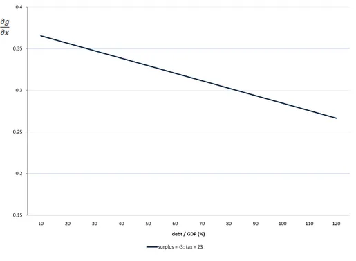
The size of the effect of productive expenditures on growth was calculated assuming a primary surplus
of -3% and a tax burden of 23%. In this scenario, the marginal effect of an increase in productive
expendi-tures by 1% of the GDP on long-term growth varies from 0.36% to 0.26% for values of the debt-to-GDP
ratio that range between 10% and 120%, as shown in Figure 4. Changes in the values of the tax burden
and the surplus shift this relationship either upwards or downwards; however, given that the coefficients
of these interactions are very small, these shifts do not occur in a perceptible way. This shows that the
interactions with the tax burden and with surplus, although they are significant and have the expected
di-rection, are not large. These results suggest that the value of the size of the debt-to-GDP ratio is the most
relevant variable for determining the effect of productive expenditures on growth, as it is quantitatively as
well as statistically significant.
6Other estimations using the system-GMM were conducted following an alternative strategy that has been used in the
Figure 4: Marginal Effect of Productive Expenditures (x) in Economic Growth
0.15 0.2 0.25 0.3 0.35 0.4
10 20 30 40 50 60 70 80 90 100 110 120
debt / GDP (%)
surplus = -3; tax = 23
3.2
Results for Mean Group Estimates
In this section, the baseline model was re-estimated while relaxing the hypothesis that the slope
parame-ters are common across countries. If this restriction was invalid, then the inferences that were performed
in the previous sections would also be invalid. The heterogeneity of the parameters among countries
is plausible because the efficiency of public expenditures can be different given alternative institutional
conditions. Therefore, given the likely importance of heterogeneous coefficients, we use the Mean Group
Estimator of Pesaran and Smith (1995) and follow the same strategy used by Bond et al. (2010); Gemmell
et al. (2011); Lee et al. (1997) for growth regressions with a panel that is similar to ours.
In simple terms, the Mean Group Estimator individually estimates the equation (15) using a two-step
GMM, using the same previously used instrument set, for each country using transformed variables by
subtracting the sample mean values for the same year from the original series, to corrects the possible
effects of common shocks, and then obtain the average of the estimated coefficients for the countries.
In our case, we individually obtained the estimated long-term effects for the countries and estimated the
robust means together with their standard errors7.
Another possible problem for the estimations is the existence of cross-sectional dependence. This
oc-curs if the economic growth of the country affects the growth of other countries, such that the residualeit
would not be independent among countries. This effect is plausible if we believe that there are spillovers
that impact technology and the accumulation of physical or human capital (Conley and Ligon, 2002) or
if the economic development of one country affects the terms of trade of the other countries (Acemoglu
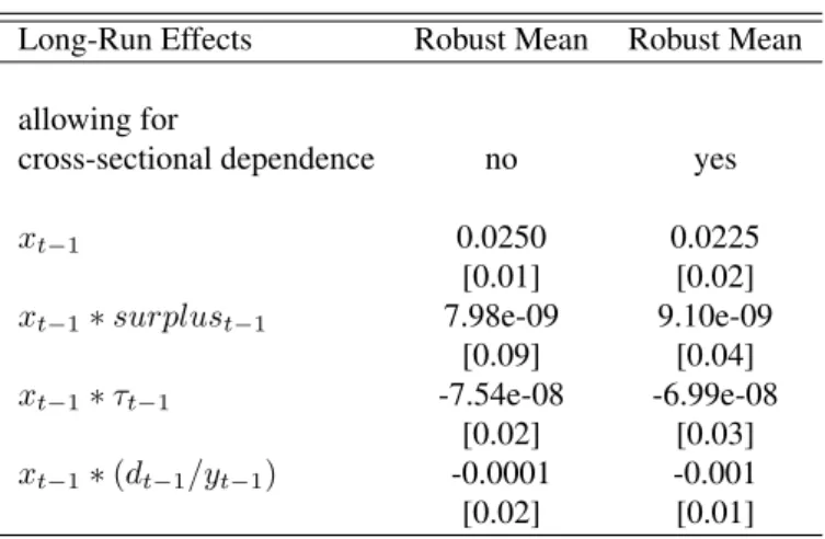
Table 2: Mean Group Estimates
Long-Run Effects Robust Mean Robust Mean
allowing for
cross-sectional dependence no yes
xt−1 0.0250 0.0225
[0.01] [0.02]
xt−1∗surplust−1 7.98e-09 9.10e-09 [0.09] [0.04]
xt−1∗τt−1 -7.54e-08 -6.99e-08 [0.02] [0.03]
xt−1∗(dt−1/yt−1) -0.0001 -0.001 [0.02] [0.01]
Notes:Robust Means are reported.p-values are in square brackets.
All specifications includegrit−1,xit−1,xit−1∗τit−1,xit−1∗surplusit−1,xit−1∗ dit−1/yit−1treated as endogenous. See table 1 for the list of instruments used (here in
deviations-from-means form)
and Ventura, 2002). To correct such a problem, we follow the procedure suggested by Pesaran (2006) of
including the annual average growth of the country as an explanatory variable. This method can also be
seen as a way to include the more flexible tendency of the individual estimations for the countries.
Table 2 depicts the results that were generated by the Mean Group Estimator of the long-term
parame-ters that were estimated from the variables of interest in the model. The columns depict the specifications
with and without the correction for cross-sectional dependence. The results depict values that are lower
in magnitude for the effect of fiscal policy on growth, showing some evidence that the pooled estimations
can show bias by not considering the heterogeneity of the parameters. Even so, all of the long-term
coef-ficients have the same signs that were previously suggested by the theoretical model and are statistically
significant. Furthermore, when calculating the marginal effect of productive spending, we obtain that this
effect becomes negative for a debt-GDP ratio above 22.5%.
As a result, we find that as more econometric problems are addressed, the effect of public debt on the
relationship between productive government expenditures and economic growth becomes more robust,
corroborating the predictions of the proposed theoretical model.
4
Conclusion
Research that seeks to estimate the effects of fiscal policy on economic growth has ignored the role of
public debt in this relationship. This paper proposed a theoretical model of endogenous growth in which
the level of the public debt-to-GDP ratio can negatively affect the effect that productive public
expen-ditures have on growth. Therein, the main conclusions of the theoretical model were tested through an
econometric model to provide evidence for the validity of this conclusion. Our empirical analysis controls
for time-invariant, country-specific heterogeneity in the growth rates. We also address endogeneity issues
and allow for heterogeneity across countries in model parameters and for cross-sectional dependences.
Our approach has enabled us to verify the effects that have already been predicted in the literature,
such as in Barro (1990), or given the indebtedness rate. Such effects represent negative consequences in
terms of direct capital accumulation, as they lead to diminishing marginal net returns of capital or savings
extracted from the economy to finance pubic expenditures.
In addition to the above effects, we were able to observe an additional effect, wherein the impact
that productive expenditures have on growth depends on the size of the debt-to-GDP ratio. This occurs
because an increase in the magnitude of productive expenditures leads to an increase in the productivity
of the economy, and thus, to an equilibrium of interest rates, as there is no decreasing marginal return
for aggregate capital in the endogenous growth models. This increase in interest rates leads to higher
government spending from debt servicing, such that as the size of the debt increases, so does the impact
from this increase on interest rates. This is why a higher debt-to-GDP ratio corresponds to a smaller
impact of productive expenditures on economic growth.
We can also understand this effect as an income transfer between generations, specifically, from the
younger generation, which has a portion of its savings invested in government securities, thus decreasing
capital accumulation in order to pay the interest on the debt of the older generation, which does not save.
In this sense, the observed effect is similar to that of the pay-as-you-go pension system in overlapping of
generation models, where income is transferred between generations and decreases the accumulation of
capital.
In addition to incorporating the effect of public debt on the relationship between productive
expen-ditures and economic growth, the model also demonstrates that increases in the size of the debt can lead
to greater economic growth, since the status quo is a healthy fiscal situation and indebtedness is
associ-ated with an increase in productive expenditures. This runs contrary to previous models, in which debt
increases always lead to decreased growth. This result shows that changes in the public debt can be
Pareto optimal, leading to benefits for all generations, which is quite different from that suggested by
endogenous models of debt, where expenditures are always unproductive.
Using the econometric specifications that were derived from the theoretical model, the main
con-clusions of the model can be established. In particular, it is clear that the omission of the interactions
between productive expenditures and the tax burden, primary surplus, and public debt, can be a source of
bias in the estimation of the effects of fiscal policies on growth. The results suggest that the size of the
debt-to-GDP ratio is the most relevant variable in determining the effect of productive expenditures on
growth, as it was found to be both quantitatively and statistically significant. Various econometric
prob-lems were addressed, wherein our findings suggest that as more econometric probprob-lems are addressed,
the effect of public debt on the relationship between productive government expenditures and economic
References
Acemoglu, D. and Ventura, J. (2002), “The world income distribution”,The Quarterly Journal of Economics, Vol.
117, pp. 659–694.
Agell, J., Ohlsson, H. and Thoursie, P. S. (2006), “Growth effects of government expenditure and taxation in rich
countries: A comment”,European Economic Review, Vol. 50, pp. 211–218.
Aschauer, D. A. (1989), “Is public expenditure productive?”,Journal of Monetary Economics, Vol. 23, pp. 177–
200.
Barro, R. J. (1990), “Government spending in a simple model of endogenous growth”,Journal of Political Economy
, Vol. 98, pp. S103–26.
Bond, S., Leblebicioglu, A. and Schiantarelli, F. (2010), “Capital accumulation and growth: a new look at the
empirical evidence”,Journal of Applied Econometrics, Vol. 25, pp. 1073–1099.
Bond, S. R., Hoeffler, A. and Temple, J. (2001), Gmm estimation of empirical growth models, CEPR Discussion
Papers 3048, C.E.P.R. Discussion Papers.
Brauninger, M. (2005), “The budget deficit, public debt, and endogenous growth”, Journal of Public Economic
Theory, Vol. 7, pp. 827–840.
Chen, B.-L. (2006), “Economic growth with an optimal public spending composition”,Oxford Economic Papers,
Vol. 58, pp. 123–136.
Conley, T. G. and Ligon, E. (2002), “Economic distance and cross-country spillovers”,Journal of Economic Growth
, Vol. 7, pp. 157–87.
Devarajan, S., Swaroop, V. and Heng-fu, Z. (1996), “The composition of public expenditure and economic growth”,
Journal of Monetary Economics, Vol. 37, pp. 313–344.
Durlauf, S. N., Johnson, P. A. and Temple, J. R. (2005), Growth econometrics,inP. Aghion and S. Durlauf, eds,
‘Handbook of Economic Growth’, Vol. 1 ofHandbook of Economic Growth, Elsevier, chapter 8, pp. 555–677.
Easterly, W. and Rebelo, S. (1993), “Fiscal policy and economic growth: An empirical investigation”,Journal of
Monetary Economics, Vol. 32, pp. 417–458.
Gemmell, N., Kneller, R. and Sanz, I. (2011), “The timing and persistence of fiscal policy impacts on growth:
Evidence from oecd countries”,Economic Journal, Vol. 121, pp. F33–F58.
Glomm, G. and Ravikumar, B. (1997), “Productive government expenditures and long-run growth”, Journal of
Economic Dynamics and Control, Vol. 21, pp. 183–204.
Gregoriou, A. and Ghosh, S. (2009), “On the heterogeneous impact of public capital and current spending on growth
across nations”,Economics Letters, Vol. 105, pp. 32–35.
Kneller, R., Bleaney, M. F. and Gemmell, N. (1999), “Fiscal policy and growth: evidence from oecd countries”,
Journal of Public Economics, Vol. 74, pp. 171–190.
Lee, K., Pesaran, M. H. and Smith, R. (1997), “Growth and convergence in multi-country empirical stochastic
solow model”,Journal of Applied Econometrics, Vol. 12, pp. 357–92.
Pesaran, M. H. (2006), “Estimation and inference in large heterogeneous panels with a multifactor error structure”,
Econometrica, Vol. 74, pp. 967–1012.
Pesaran, M. H. and Smith, R. (1995), “Estimating long-run relationships from dynamic heterogeneous panels”,
Journal of Econometrics, Vol. 68, pp. 79–113.
Saint-Paul, G. (1992), “Fiscal policy in an endogenous growth model”,The Quarterly Journal of Economics, Vol.
Table 3: Descriptive Statistics (%)
Median Mean Standard Deviation Min. Max. Per Capita GDP Growth 2.50 2.27 5.6 -41.11 56.40 Productive Expenditures / GDP 7.35 8.33 4.03 0.90 30.84 Income Tax / GDP 5.46 6.71 4.63 0.47 27.88 Surplus / GDP -3.15 -3.93 6.18 -61.14 62.18 Debt / GDP 44.07 56.75 58.19 0.38 637.52
Table 4: List of Countries