Demand, supply and markup fluctuations

REM WORKING PAPER SERIES

Demand, Supply and Markup Fluctuations

Carlos D. Santos, Luís F. Costa and Paulo Brito

REM Working Paper 041-2018

June 2018

REM – Research in Economics and Mathematics

1249-078 Lisboa, Portugal

ISSN 2184-108X

Any opinions expressed are those of the authors and not those of REM. Short, up to two paragraphs can be cited provided that full credit is given to the authors.

Demand, Supply and Markup Fluctuations

Carlos D. Santos

, Luís F. Costa

, and Paulo Brito

08.06.2018

Abstract

Markup cyclicality has been central for debating policy e¤ectiveness and understanding business cycle ‡uctuations. However, there are two empiri-cal challenges: separating supply (TFP) from demand shocks, and properly measuring the markups. In this article, we use a panel of Portuguese man-ufacturing …rms for 2004-2014. Since it contains information on product-level prices, we can separate supply from demand shocks. We overcome the markup measurement by using the share of intermediate inputs on revenues, instead of the labor share. Our results suggest that markups are pro-cyclical with TFP shocks, and counter-cyclical with demand shocks. We also show that labor-based markups are pro-cyclical.

Financial support by FCT (Fundação para a Ciência e a Tecnologia), Portugal, is grate-fully acknowledged. This article is part of the Strategic Projects UID/ECO/00436/2013 and UID/ECO/00124/2013, and it is also …nanced by POR Lisboa under the project LISBOA-01-0145-FEDER-007722. Carlos Santos gratefully acknowledges FCT research fellowship CONT-DOUT/114/UECE/436/10692/1/2008 under the programme Ciência 2008. We would like to thank Vasco Matias and André Silva for their research assistance, and INE (Statistics Portugal), especially So…a Pacheco, M. Arminda Costa, and Carlos Coimbra, for their help with microdata. Comments and suggestions by Huw Dixon, Huiyu Li, Gauthier Vermandel, and by the partic-ipants at the Lisbon Macro Club workshop, T2M Theories and Methods in Macroeconomics conference (Lisbon), 11th World Congress of the Econometric Society (Montréal), 30th Annual Congress of the European Economic Association (Mannheim), 8th Meeting of the Portuguese Economic Journal (Braga) and at at seminars in EIEF (Rome), Cardi¤ University, and ISEG of ULisboa (Lisbon) are gratefully acknowledged. The usual disclaimer applies.

y_{Nova School of Business and Economics, UNL, 1099-032 Lisboa, Portugal.}

z_{ISEG - Lisbon School of Economics & Management, Universidade de Lisboa, Rua do}

Quelhas 6, 1200-781 Lisboa, Portugal.

x_{REM – Research in Economics and Mathematics, UECE – Research Unit on}

Keywords: Markups, Demand Shocks, TFP shocks JEL classification: C23, E32, L16, L22

1

Introduction

How markups move, in response to what, and why, is almost terra incognita for macro.

In: Blanchard (2009)1 The cyclical behavior of markups, that is, the wedge between prices and mar-ginal costs, has been at the center of the macroeconomic debate on the origins of business-cycle ‡uctuations and policy e¤ectiveness. Hall (2009), when analyzing the role of varying markups in …scal-policy e¤ectiveness refers: "models that de-liver higher multipliers feature a decline in the markup ratio of price over cost when output rises (...)".2

In theory, markups may ‡uctuate endogenously with the business cycle due to sluggish price adjustment (undesired endogenous markups), or to deeper motives a¤ecting the price-elasticity of demand faced by individual producers (desired en-dogenous markups) - for a comprehensive survey see Rotemberg and Woodford (1999), and section 2 for a brief analysis of the relevant literature.

However, theory alone is not insu¢ cient to determine by how much prices, and marginal costs, will move relative to each other along the business cycle. That is why empirical evidence is much needed.

Yet, the empirical evidence is mixed. First and foremost, the inconclusive results are related with the fact that separating demand and supply shocks is a di¢ cult task in the absence of separate price and quantity data. Thus, if supply and demand shocks exhibit di¤erent cyclical patterns, a "weighted average" of the two may exhibit either pro- or counter-cyclical behavior, depending on which shock is more prevalent. Furthermore, for data availability, the literature has used the labor share to construct the markups. Labor is subject to adjustment cost, which

1_{Op. cit. p. 220.}

create a wedge between the markup and the labor share. Markup will thus be mismeasured and perhaps even exhibit the opposite cyclicality3.

In this article, we make use of the availability of product-level prices for a panel of Portuguese manufacturing …rms over the period 2004-2014, a period during which the country faced two of the main crisis in the recent past - the 2008-2009 …nancial crisis and the 2010-2011 European sovereign debt crisis. We merge these prices with the yearly census data containing balance sheet and income statement data. The detail of the data allows us to estimate a structural model of demand and production (supply side), and thus obtain separate measures of demand and supply (TFP) shocks for each individual company. On the supply side, we follow DeLoecker et al. (2016) to obtain production-function estimates for multi-product …rms. This method also uses materials as the pivotal input to measure markups. Furthermore, it also allows us to control for unobserved input quality. On the demand side, we use a utility-based nested-homothetic demand function for a rep-resentative consumer, which is somewhat inspired by Foster et al. (2016). Since we impose very few restrictions, non-constant elasticities can be obtained for demand functions faced by each producer. The methodology used here can be easily ex-tended to other countries and periods with the expansion of access by researchers to detailed …rm-product micro information where prices are observed.

Our results show that markups are countercyclical with the demand shocks while they are pro-cyclical with supply shocks. The explanation for the behavior rests with the cost structure. When faced with a positive demand shock, companies increase prices slightly. However, the short run upward slopping marginal cost curves (due to the existence of …xed inputs such as capital and possibly also labor) implies an increase in costs. The price increase do not cover the cost increase which results in a reduction of the markup. We also show that multi-product …rms exhibit a smaller degree of cyclicality with demand shocks, but not with supply shocks. This suggests that multi-product …rms have a more ‡exible cost structure that allows costs to be more easily adjusted as a response to demand shocks. We believe this is due to the reallocation of inputs across products, but we do not have product-speci…c data on inputs to test this explanation.

3_{Nekarda and Ramey (2013) correctly point out that it is the marginal wage and not the}

av-erage wage that is the adequate measure do determine marginal costs. Rotemberg and Woodford (1999) present other types of labor frictions that also in‡uence the markup level and cyclicality.

Our …ndings have implications for macroeconomic policy. When facing a re-cession, while stimulating aggregate demand, governments and central banks may bene…t from an e¢ ciency gain from lower markups. "Hence recessions are not only bad because output is low, but also because microeconomic distortions are greater. This suggests that stabilization of output at a high level is desirable because it reduces these distortions" (Rotemberg and Saloner (1986))4_.

Empiri-cally, without separate measures for markup and productivity, this e¤ect looks like (is observationally equivalent to) a positive productivity shock, while it is actu-ally an e¢ ciency gain from reduced markups. Confounding the markup e¢ ciency (demand-driven) gain with a productivity shock, leads to an underestimation of macroeconomic policy e¤ectiveness. In addition, these stronger multiplier e¤ects may be understated for samples of large and diversi…ed …rms that are regularly used for empirical analysis (such as COMPUSTAT), as diversi…ed …rms smooth markup responses by reallocating inputs (and costs) across di¤erent products. As for Portugal, the empirical evidence suggests that the 2010-4 …nancial crisis, that arguably started with a negative demand shock, may have been exacerbated by the side e¤ects of …scal consolidation, leading to a signi…cant increase in the markups across the economy.

The article is organized as follows. In section 2 we present the related liter-ature. Section 3 provides some preliminary macro and micro data and empirical motivation. Section 4 provides a birds-eye view of the problem. In section 5 we present the model an its components. Section 6 describes the data and reports the empirical results of the estimation procedures. Section 7 analyses the markups and their cyclicality. Finally, section 8 concludes.

2

Related literature

This article is related to several earlier contributions. Since our intent is not to produce a survey, but to supply evidence on the cyclicality of markups with demand and supply shocks, we summarize some of the more important contributions below. On the theory side, there is a number of so-called endogenous-markup models. The undesired type is present in macroeconomic models that assume sticky prices

as state-dependent models of the menu-costs sort, e.g. Mankiw (1985), and time-dependent models as Calvo (1983), Rotemberg (1982) or the sticky-information model of Mankiw and Reis (2002). The desired type comprises a large number of reasons including more general preferences outside the CES benchmark as in Bilbiie et al. (2012), Feenstra (2003) or Ravn et al. (2008), heterogeneity of demand as in Galí (1994) or Edmond and Veldkamp (2009), intra-industrial competition, that may be potential or existing, as in Barro and Tenreyro (2006), Costa (2004) or Rotemberg and Woodford (1991), feedback e¤ects as in Jaimovich (2007), amongst other motives. For a survey see Rotemberg and Woodford (1999).

On the empirical side of the literature, Rotemberg and Woodford (1999) use the evidence on the cyclical behavior of the labor share in total income, a macroeco-nomic approach, to conclude that average markups are unconditionally counter-cyclical, so they have to be counter-cyclical with demand shocks. Martins and Scarpetta (2002) use a di¤erent approach, slightly related to Industrial Organiza-tion (IO), but reach similar conclusions for a sample of industries in G5 countries. More recently, Juessen and Linnemann (2012) provide evidence of counter-cyclical markups for a panel of 19 OECD countries; Afonso and Costa (2013) …nd that markups are counter-cyclical with …scal shocks for 6 out of 14 OECD countries and pro-cyclical for 4 of them; Nekarda and Ramey (2013) …nd either acyclic or pro-cyclical markups with demand shocks for US industries. Finally, Bils et al. (2018) use BLS and KLEMS data for the US and "…nd price markup movements are at least as cyclical as wage markup movements."

A strand of literature, closer to our article, has been recently developed using micro data to answer some of the relevant macro questions. Foster et al. (2013) uses US Census data to obtain separate estimates of the demand and productivity components and their e¤ect on …rm growth. The US Census data is at a 5 year frequency and is thus not very informative about short run ‡uctuations. On the other hand, Gilchrist et al. (2014) use monthly product level prices merged with quarterly data for a sample of large …rms from COMPUSTAT to look at how …-nancial behavior of …rms in‡uences the price responses. Pozzi and Schivardi (2016) use the …rms’ self-reported price changes to construct a …rm-speci…c price index and purge the TFP measure from demand shocks and evaluate their importance for …rm growth. To address the problem of multi-product …rms, DeLoecker et al.

(2016) develop a methodology to estimate production and productivity estimates for multi-product …rms, and study the e¤ect of trade liberalization on prices and markups of companies in India. They …nd evidence of increasing markups after trade liberalization due to the limited pass-through of cost savings into prices. This limits the gains from trade, at least in the short run. Finally, Hong (2017) uses Amadeus data for France, Germany, Italy, and Spain to estimate unconditional elasticities of markups to GDP.

3

Some preliminary evidence

We start with a preliminary analysis of the cyclical behavior of markups in the Portuguese economy from 2004 to 2014 using both aggregated and disaggregated data. A detailed description of the data is contained in Appendix A.2. The data is particularly useful as it overlaps the two largest crises in the last three decades: the 2008-2009 …nancial crisis and the 2010-2011 European sovereign debt crisis.

3.1

Macro evidence

The economy-wide markup in year t ( _t), is the weighted geometric mean of the markup ( _it) for each individual …rm i = 1; :::; n:

t= nt Y i=1 !it it ,

where nt is the total number of …rms in the census in year t and !it= yit=

Pnt

i=1yit

is the share of …rm i in total sales (production value) in year t, with yitrepresenting

the sales (total revenue) of …rm i in year t. The growth rate for the average markup is approximately given by5 ln _t' nt X i=1 (ln _it !it+ !it ln it) .

The markup of …rm i at time t is the ratio of price (pit) over marginal cost (cit):

it =

pit

cit

. (1)

For the case where the production function is Cobb-Douglas, including labor (`) and materials (m) with constant parameters over time, then ln _it = ln sx_it, where sx

it is the ratio of the cost of input x = `; m to total revenue.6 This is

a …rst-order approximation which we will relax later. Finally, letting weights be approximately constant ( !it ' 0), we obtain a measure for the growth rate of the

average markup: ln x_{t '} nt X i=1 !it ln sxit; x2 f`; mg .

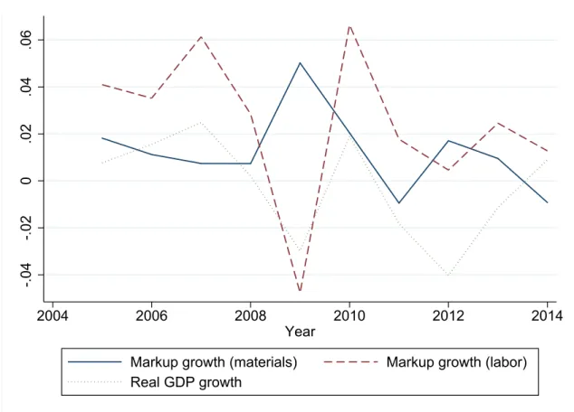
The growth rates of the input share (materials and labor) in the 2004-2014 period are calculated using the census data from IES (Informação Empresarial Simpli…cada7_{), which contains all non-…nancial companies. Figure 1 depicts the}

average markups (labor- and materials-based) and real GDP (g) growth rates. Markups are counter-cyclical with respect to GDP when materials are used to measure it; however, they are pro-cyclical when labor is used instead. Overall, the pattern is explained by the high responsiveness of intermediate inputs and low responsiveness of labor relative to revenues.

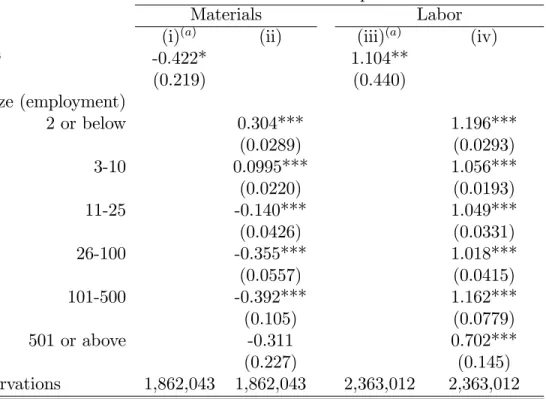
Table 1 suggests that on average a 1 per cent increase in GDP is associated with a 0.4 per cent reduction in markups when we use the materials-based measure. However, the same 1 per cent increase in GDP is associated with a 1 per cent increase in markups, when we use the labor-based measure. This rough elasticity is not the same across …rm size (employment) classes. Smaller …rms exhibit a positive association with GDP growth, with micro …rms (2 or less employees) reporting an elasticity of 0.3. The correlations become negative for …rms above 10 employees and level o¤ for really large …rms (above 500 employees). No discernible patterns exists when markups are measured via labor.

These results compare for example with Bils et al. (2018) and Hong (2017), who estimate markup elasticities with respect to GDP in the order of (negative) 0.9-1.2.

6_{These are the most common measures of markups considered in the literature.}

-.04 -.02 0 .02 .04 .06 2004 2006 2008 2010 2012 2014 Year

Markup growth (materials) Markup growth (labor)

Real GDP growth

Figure 1: Economy-wide time-series for average markups (labor- and materials-based) and GDP growth. Source: SCIE (Census).

Table 1: Reduced-form GDP elasticities for …rm (labor- and materials-based) markups. Source: SCIE (Census).

Markup

Materials Labor (i)(a) _{(ii) (iii)}(a) _(iv)

lng -0.422* 1.104** (0.219) (0.440) by size (employment) 2 or below 0.304*** 1.196*** (0.0289) (0.0293) 3-10 0.0995*** 1.056*** (0.0220) (0.0193) 11-25 -0.140*** 1.049*** (0.0426) (0.0331) 26-100 -0.355*** 1.018*** (0.0557) (0.0415) 101-500 -0.392*** 1.162*** (0.105) (0.0779) 501 or above -0.311 0.702*** (0.227) (0.145) Observations 1,862,043 1,862,043 2,363,012 2,363,012 Notes: OLS results from the regression of growth rates of markups

on growth rates of GDP. Markup growth truncated at 2. (a) Regressions are weighted by revenues. Standard errors (in brackets) clustered by …rm and year. Signi…cance levels: 1 per cent (***), 5 per cent (**), and 10 per cent (*).

Bils et al. (2018) use BLS and KLEMS data for the US. Hong (2017) uses a sample of mostly very large companies, covered by Amadeus (for France, Germany, Italy, and Spain) which can explain the larger estimates.

Unfortunately, the observed heterogeneity in responses implies that the GDP elasticity of markups depends on market structure so that we can not produce one "magic" number to educate policy makers. Furthermore, such simple regression results also abstract from two fundamental questions. First, the origin of the shocks to GDP: demand vs. supply. Fluctuations due to supply-side (productivity) shocks can generate the opposite response for markups when compared to those generated by demand-side shocks. Second, the mechanism by which markups react

to such shocks requires we add some structure to study the problem. Quoting Rotemberg and Saloner (1986), who …nd a negative e¤ect of GNP growth on price growth for the US Cement industry: "These results are of course not conclusive. First, it is possible that increases in GNP lower the demand for cement relative to that for other goods. Without a structural model, (...), this question cannot be completely settled."8 _{Three important elements explain how markups respond:}

prices, quantities, and marginal costs. As we will see in the remaining of the article, this distinction is fundamental to understand the source of markup ‡uctuations.

3.2

Micro evidence

Let us start by decomposing the e¤ects on prices and marginal costs at the mi-cro level. First, we use the data from IAPI (Inquérito Anual à Produção Indus-trial9_{), a survey that collects product-level annual information on revenues and}

sales (quantities) of industrial goods to construct the 9-digit prices for each indi-vidual product-…rm as the ratio of revenues to sales. We can also obtain direct proxies of the marginal cost for the two inputs, by computing the ratio of the total expenditure in intermediate inputs (and the wage bill) to physical output. A large ratio means that, on average, more inputs are required to produce a unit of output, e.g. if ‡our is used in larger amounts to produce x kg of bread, the marginal cost of producing bread is higher.

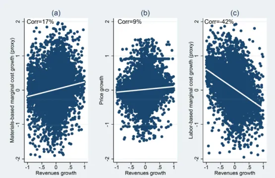
Figure 2 illustrates how the growth of prices and marginal costs vary with the growth of revenues. All variables are in …rst di¤erences of logs, so that these are e¤ectively within-…rm (year on year) variations. First, panel (a) shows that the growth of (materials-based) marginal costs increases with the growth of revenues (the correlation is 17%), while panel (b) shows that prices are relatively unrespon-sive (the correlation is 9%). On the other hand, we can see in panel (c) that (wage-based) marginal cost growth decreases with revenue growth (the correlation is -42%).

These patterns produce an expected increase in labor-based markups and an expected decrease in materials-based markups to revenue growth. The di¤erent response of the two measures of marginal costs, together with the prices changes,

8_{Op. cit. p. 399}

are fundamental to explain the behavior of markups. In particular, the existence of predetermined factors such as capital and labor, generate an upward-sloping marginal cost function. Adding relatively mild price adjustments and stronger quantity responses generates the observed patterns for the markups.

Figure 2: Marginal cost and price vs. revenue growth. Source: SCIE (Census) and IAPI.

While this evidence rationalizes the mechanism explaining markup cyclicality, we have still not addressed the source of the shocks: demand vs. supply. However, marginal costs and prices are expected to respond di¤erently. While both prices and marginal costs are expected to increase with a positive demand shock, both are expected to decrease with a positive productivity shock. The simple framework presented in the following section introduces both demand and supply levels, and allows us to interpret the basic evidence through the lens of a structural model. Later, we will use our product and …rm information to isolate the two shocks.

4

A birds-eye view on the e¤ects of shocks on

markups

The product-…rm markup is a function of …rm-speci…c TFP (a), and …rm-product speci…c demand ( ) shifters. Before delving into the measurement issues related to the three variables ( , a, and ), it is useful to understand the nature of the response of markups to the two shifters. The individual producer faces an inverse demand function generically given by p = P (q; ; ), where q represents the quantity sold, Pq < 0, and P > 0.10 Similarly, the marginal cost function given by c =

C (q; a; ), where Cq 0, and Ca < 0. Finally, the markup is M (q; ; a; ) =

P (q; ; ) =C (q; a; )_{. While function M ( ) captures the direct e¤ect of productivity} and demand shocks, there are also the indirect e¤ects that, in equilibrium, cause changes in the quantity produced q.

For any product, the revenue obtained equals price times quantity, y = Y (q; ; ) = pq. The regularity conditions imply that marginal revenue Yq = Pq(q; ; ) q +

P (q; ; ) > 0is decreasing in q (i.e. Yqq = 2Pq+Pqqq < 0) and is increasing in (i.e.

Yq = P + Pq q > 0). Consequently, from the optimality condition Yq = c,11 we

ob-tain q = Q ( ; a; ), where Q = Yq = (Cq Yqq) > 0, and Qa = Ca= (Cq Yqq) > 0.

Markups are thus a function of the levels of productivity and demand, either by a direct e¤ect to the marginal-cost and demand demand functions, or by an indirect e¤ect to the (optimal) production level. We can decompose these two channels. A change in total factor productivity (TFP), has an impact on the markup that can be summarized by the following partial derivative12_:

a= PqQa c CqQa c | {z } indirect e¤ect =_Mq Qa + Ca c | {z } direct e¤ect =_Ma + . (2)

There is a positive direct e¤ect of an increase in TFP as it reduces the marginal

10_{We denote partial derivatives of function g = G (x1; x2) as Gx}

1

@G

@x1 and Gx1x2

@2G

@x1@x2.

11_{In fact, we do not need to assume optimal pricing here. Cost minimisation together with any}

(sub-)optimal production rule would su¢ ce.

cost ( Ca=c > 0). However, there are two indirect e¤ects with negative sign,

due to the increase in production: (i) the price decreases (PqQa=c < 0) and (ii)

the marginal cost increases ( CqQa=c < 0). Despite the fact that theoretically a

can be positive or negative, there is a consensus in postulating it to be positive, i.e. that markups are pro-cyclical with TFP shocks. The e¤ect operating through the increase in production (reduction in price and increase in marginal cost) is not su¢ cient to counteract the direct reduction in marginal cost. This is equivalent to assume that the absolute value for the elasticity of the marginal cost with respect to productivity, Ca_,13 _{is large enough, and the following condition holds:}

a > 0, Ca > Cq Pq Qa > 0.

For demand, a change in the level leads to

= PqQ c CqQ c | {z } indirect e¤ect =_Mq Q + +P c |{z} direct e¤ect =_M + . (3)

There is a positive direct e¤ect on the price via shift in the demand (P =c > 0) and two negative indirect e¤ects, due to an increase in production: (i) the price decreases (PqQ =c < 0) and (ii) the marginal cost increases ( CqQ =c <

0). There is no consensus about the net e¤ect of a positive demand shock on markups. Markups are counter-cyclical, if the e¤ect operating through the increase in production (reduction in price and increase in marginal cost) is su¢ cient to counteract the direct increase in prices (i.e. if the price adjustment is relatively small). Thus, markups are counter-cyclical with demand shocks ( < 0) if the ratio of the elasticities of the inverse demand function and of output, both with respect to the demand shock ( P ₌ Q _{> 0), is smaller than the di¤erence of the}

elasticities of marginal cost relative to demand for output changes ( Cq Pq _{> 0),}

and the following condition holds:

13_{From now on we denote by} G_{x1 G}

< 0 _, P = Q < Cq Pq _.

Otherwise, they are pro-cyclical with these shocks.

Next we present our approach for estimating the markups, the TFP, and the demand shocks. The results, using two rich databases for Portuguese …rms, are reported in section 6. In section 7 we report numerical estimates of the elasticities

a and .

5

The model

In this section, we provide the theoretical elements to the problem of uncovering markup cyclicality, brie‡y analyzed above. We use a measure of markups adapted to our dataset and present a speci…cation for the demand and production functions, allowing for the separate measurement of the TFP and demand shocks. Our …nal goal is to calculate the markup elasticities in Equations 2 and 3.

First, the production technology to produce good j by …rm i at time t is

ln qijt = ln Fj(kijt; `ijt; mijt) + ait , (4)

where k represents the stock of physical capital, ` is the labor input, and m is an intermediate input (materials). The production function parameters are product-speci…c, and are the same for all …rms producing good j. We follow DeLoecker et al. (2016) and let inputs be product-…rm speci…c, while TFP (ait) is shared across all

products within the …rm. In this case, inputs and productivity are unobserved for two reasons: (i) we can only observe input usage at the …rm level and (ii) input quality is not observed. We will address both issues below.

Second, similarly to Foster et al. (2016) we assume that the quantity demand of good j produced by …rm i at time t is

ln qijt = ln Dij(pijt; pjt; pt; gt; ijt) + ijt , (5)

where pijt is its price, pjt is the average price of product j, pt is the aggregate

price index, gt is real GDP, ijt is the quality level, and ijt is the idiosyncratic

that …rm i retains some market power over its product, although it operates in a competitive environment with other …rms. All the arguments in Equation 5 are observed, except for the demand level and product quality.

Estimation proceeds in three steps. First, we estimate the production function in Equation 4 using data for single-product …rms. Second, using the estimated pro-duction function parameters we calculate the input-shares for each multi-product …rm together with the …rm-level TFP. This step involves only solving, not estimat-ing, a system of equations. Finally, we use the calculated TFP as an instrument to estimate the demand function in Equation 5 for each product-…rm. Demand shocks are obtained as the residuals from this equation.

5.1

Markups measurement

We now start by addressing the measurement of markups. Consider Equation 4, where all inputs are substitutes, and at least one input is freely adjustable and not subject to adjustment costs. Furthermore, let …rms be price takers in input markets, so that r is the rental on capital, w is the wage rate, and b is the price of materials, all exogenous. This assumption is important and is discussed at length in DeLoecker et al. (2016).

Under these conditions, an optimizing …rm faces a marginal cost of producing good j equal to the ratio between the price of an input (zx

2 fr; w; bg) and its marginal product in the production of j (Fx;ijt with x 2 fk; `; mg), i.e. cijt =

zx

t=Fx;ijt. Therefore, the markup of …rm i in the production of j at time t is given

by ijt= Fx ijt sx ijt , (6) where sx

ijt = zxxijt=yijt is the share of the cost of input x on total revenues for

product j (yijt= pijtqijt). The elasticity Fijtx, that is, the ratio between the marginal

and the average product of input x in the production of j, depends on the functional form assumed for the production function Fj( ). The elasticity is not observed in

the data and must be estimated via production function, which we assume to be the same for all …rms producing j. For single-product …rms, the share sx is observable for labor and materials. For multi-product …rms, we need to calculate the allocation

of intermediate inputs for …rm i across all products. From the estimated parameters for the production function, Fj( ) from Equation 4, we obtain an estimate of the

input elasticity. The markup can then be constructed as speci…ed in Equation 6 using the input share data - see section 7.

While earlier contributions used labor input to measure markups in Equation 6, we use intermediate inputs instead. In addition to data availability, the main reason is that labor tends to behave as a dynamic input subject to short-run adjustment costs (hiring and …ring costs) which can be problematic and lead to incorrect results.

5.1.1 The troubles with input shares

An important share of the literature assumes that the production function is (ap-proximately) Cobb-Douglas and so the input elasticities ( Fx

ijt) become constant.

In this case, the only variation in markups will be from variation in the revenue share of the variable input. But how do shares respond to quantities? If we assume the producer is price taker in the market for input x, considering that the optimal usage of this input is given by x = X (q; ) with Xq > 0, an increase in production

will lead to @sx @q = sx q Xq 1 _{. (7)}

Thus, considering that 1= 2 (0; 1), the cyclicality of the input share depends on how much this input utilization varies with production. If all inputs are equal-ity ‡exible, optimalequal-ity conditions will lead to similar time series for input shares. However, the presence of frictions in input markets leads to the need to alter Equa-tion 6 in order to re‡ect distorted time series for input shares. This is particularly pungent when labor is used to measure markups, as shown by Rotemberg and Woodford (1999), or more recently by Nekarda and Ramey (2011).

An illustrative example may help us to clarify this point. Assume there are con-vex costs of adjusting labor from its current level. In that case, the elasticity Lq

becomes small and it is more likely to obtain an acyclical or even counter-cyclical labor share, that is, an acyclical or even pro-cyclical markup measure. Notwith-standing, changes in labor costs are clearly not the best indicators of changes in the marginal cost for this case. This is consistent with our empirical results using

labor share to measure the markup. The restrictive labor legislation in Portugal generates pro-cyclical results, when markups are calculated using the labor share. This is because the labor share does not equate to the marginal return to labor, thus creating a wedge between the share and the elasticity. The case becomes even more problematic when adjustment costs are non-convex.

Furthermore, when producers are not price takers in the labor market, e.g. in an e¢ ciency-wages model, and face an upward-slopping labor supply w = W (`; ) with W` > 0, the expression in brackets on the right-hand side of Equation 7

becomes Lq _{1 +} W` 1_{. In this case, a fully-‡exible labor input produces more}

pro-cyclical (counter-cyclical) labor shares (markups) than the real ones, using a corrected measure.

Consequently, we use materials to measure markups instead of labor, as these inputs are more likely to be used in a ‡exible manner than labor in the short run. One objection that may be raised to this strategy is that materials are a composite of several goods and services, with no clear quantity and price measures to be obtained in the data. This objection is a real one, despite the fact that labor is not an homogeneous input either. Our assumption is that the composition of the materials basket is stable for a given technology, just like for labor.

5.2

Demand function

We now deal with estimating Equation 5 and obtaining the …rm-speci…c demand shifter. There is a standard endogeneity problem due to the presence of the price pijt as an argument. We follow an identi…cation strategy similar Olley and Pakes

(1996) by letting the demand shifter ( ijt) follow a Markovian process. The process

can take any order , but due to the short time dimension of our panel we will use a …rst-order case.

Assumption 5.1 The demand level follows a separable exogenous …rst-order Markov-ian process:

ijt = ( ijt 1) + ijt , (8)

5.2.1 Benchmark case: Nested-homothetic demand function

In industrial sectors, companies operate both in consumer markets (B2C) and intermediate markets (B2B). For example, bread or pastries are sold directly to …nal consumer, via retailer or to other companies like restaurants, hotels or cafés. For simplicity, we assume that the demand for good j is well represented by a consumer with homogeneous-of-degree-one CES preferences for classes of goods organized in baskets (we will use two-digit sectors) and then a homothetic-subutility function representing the preferences over individual goods (we will use nine-digit products). The demand for good j sold by …rm i at time t in Equation 5 can thus be represented by14 ln (qijt) = 0+ 1ln pjt pt + 2ln (gt) + d pijt pjt ijt+ ijt , (9)

Function d ( ), which stems from the nested homothetic preferences, is decreasing and can be approximated by a cubic polynomial:

d pijt pjt = 1ln pijt pjt + 2ln2 pijt pjt + 3ln3 pijt pjt ,

providing us enough ‡exibility to accommodate a wide range of endogenous-markup models.

Notice that this representative-consumer model includes an intra-product com-petition component represented by pij=pj, an inter-product competition component

represented by pj=p, a proxy for macroeconomic shocks given by g, dynamic

de-mand (persistence) and a series of idiosyncratic shocks represented by . The quality shifter ( ijt) is estimated from the production function, following the

ap-proach used in DeLoecker et al. (2016), that we outline in section 5.4.

Given the Markovian assumption for ijt, all information at t 1 becomes

orthogonal to the news component ( _ijt), as well as TFP shocks in period t. Note that this assumption still allows for the TFP level (ait) to be correlated with the

demand level ( ijt). Thus, we can write the following moment condition:

E( _{ijtjZ) = 0 ,}

and estimate Equation 9 by GMM. The exact set of instruments (Z) is detailed in the empirical section and includes current and lagged TFP, labor, capital, industry prices, and the estimated measure of input quality, together with lagged own prices.

5.3

Production function: TFP

To obtain the …rm-level TFP (ait), we estimate Equation 4. Before we consider

the separation between single-product vs. multi-product …rms and quantity vs. quality, in order to obtain valid estimates of ait, we have to deal with the problems

of endogeneity, identi…cation, and speci…cation of the production function.

5.3.1 Input endogeneity

Potential endogeneity exists in Equation 4 due to the fact that TFP is an unob-served state variable correlated with inputs. We address endogeneity in a similar way to what was done for demand: by using the method proposed by Olley and Pakes (1996), that introduces a Markovian assumption on the TFP process. A problem with this approach has been raised by Bond and Soderbom (2005) and Gandhi et al. (2013). This is because, conditional on all state variables and unob-served TFP, there is no variation left in intermediate inputs to adopt the inversion method developed by Levinsohn and Petrin (2003). The parameters in the pro-duction function are thus not identi…ed. We show how to regain identi…cation by allowing persistent shocks to demand. The idea is to have a second source of vari-ation in materials, originated on the demand side, a point we discuss in detail in the next subsection.

In order to estimate Equation 4, we assume that function Fj( )is the same for

all producers of good j, including producer i. For simplicity, we ignore product (j) and producer (i) subscripts, whenever they are not required to understand the problem.

Assumption 5.2 TFP is a separable exogenous -order Markovian process:

ait= (ln ai;t 1; ::; ln ai;t ) + ait , (10)

Henceforth, we set = 1. While this is not strictly necessary, a larger would require longer time spans than the ones available in the dataset for estimation purposes. Under this condition, the production function in 4 can be written as

ln qijt= ln F (kijt; `ijt; mijt)+ (ln qij;t 1 ln F (kij;t 1; `ij:t 1; mij;t 1))+ ait . (11)

From assumption 5.2, we know that ait is orthogonal to any variable chosen at

or before period t 1 - see Blundell and Powell (2004) and Hu and Shum (2012). Thus, functions of (qij;t 1; kij;t 1; `ij;t 1; mij;t 1) are valid instruments. Intuitively,

qij;t 1 traces out function ( )while (kij;t 1; `ij;t 1; mij;t 1)trace out function F ( ).

Pre-determined variables are also valid instruments - e.g. the capital stock and the labor input, which are chosen in period t 1.15 _{Thus, we can derive the following}

moment conditions from Equation 11 and estimate it using GMM:

E 0 B B B B B B @ a it 2 6 6 6 6 6 6 4 Z_{ij;t 1}1 :: Z_{ij;t 1}N kijt `ijt 3 7 7 7 7 7 7 5 1 C C C C C C A = 0 , (12)

where Zij;t 1= qij;t 1 kij;t 1 `ij;t 1 mij;t 1 >

and Z_{ij;t 1}n = Zij;t 1 Zij;t 1n 1 =

Zij;t 1 ::: Zij;t 1

| {z }

ntimes

, for n = 1; :::; N , is the Kronecker self-product of order n. Note that we assume capital and labor are both pre-determined so that their choice is orthogonal to the "news" shock to TFP, a_it.16

5.3.2 Identi…cation

A potential identi…cation problem to the estimation of Equation 4 arises from the absence of variation in mijt, once we condition it on the set of pre-determined

15_{Violations of the Markov assumption generate serial correlation in} a

it and the identifying

condition would become invalid, i.e. variables chosen at or before period t 1 are correlated with

a

itand are no longer valid instruments. This could be addressed using a second-order (or higher)

Markov process and longer lags as instruments.

16_{We also estimated the model with endogenous labor, in which case `}

ijtdrops from the moment

variables (kijt; `ijt; ait) - see Bond and Soderbom (2005) and Gandhi et al. (2013).

This problem emerges from the optimality condition, as intermediate inputs are a direct function of the state variables, mijt = M (kijt; `ijt; ait). Conditional on the

state variables (kijt; `ijt; ait), lagged instruments do not have any informative power

about mijt and, as such, the production function coe¢ cients are not identi…ed.

However, once we allow for two unobserved shifters and introduce the level of de-mand ijt into our model, the optimality condition for intermediate inputs becomes

a function of it: mijt = M (kijt; `ijt; ait; ijt). Therefore, considering that ijt is

as-sumed to be serially correlated, lagged values of mijt (conditional on kijt; `ijt; ait)

are informative for the current values of mijt, which restores identi…cation of the

production-function coe¢ cients.

5.3.3 Benchmark case: Translog production function

Using a second-order approximation to the production function, Equation 4 takes the standard translog form:

ln q = >x+ x> x+ a , (13) = 0 B @ k ` m 1 C A , x = 0 B @ ln k ln ` ln m 1 C A , = 0 B @ kk 2k` km 2 k` 2 `` `m2 km 2 `m 2 mm 1 C A .

The elasticity in Equation 6 is a linear function of input utilization Fm

ijt = m +

kmln k + `mln ` + 2 mmln m, so that we can obtain the level of t simply by

dividing this elasticity by the input share smt .17

As for the ( )function, we use a linear approximation:

(ai;t 1) aai;t 1 .

Thus, the benchmark equation to be estimated is

17_{And if labor is fully ‡exible, the labor-based markup is given by dividing the elasticity}

F`

ln qijt= >xijt+ x>t xijt+ a ln qij;t 1 >xij;t 1 x>ij;t 1 xij;t 1 + a

it . (14)

Notice that this equation cannot be estimated by OLS, as mijt is endogenous.

Thus, we use the GMM estimator de…ned above.

5.4

Multi-product …rms and input quality

The existence of price-level data and multi-product …rms introduces two new mea-surability concerns to the estimation of Equation 4. First, a large proportion of …rms produce more than one product and we do not observe the inputs allocated to each individual product. We only observe the aggregate input utilization by …rm i. Second, except for labor, the values of inputs used by …rm i are observed, instead of the quantities of each input. Multi-production further introduces a potential bias due to the existence of economies of scope, restricting rivalry in input utiliza-tion among di¤erent goods. Allocating inputs using the share of total revenues originated from product j does not address this bias. The presence of economies of scope is permitted, by letting total factor productivity vary across single and multi-product …rms, while still maintaining the same cost function across all companies. A di¤erent, but not necessarily independent, bias is related to companies using in-puts of varying quality to produce a given output. This is particularly problematic when we measure output in quantities. While the problem is also present when output is measured in revenues, it becomes less apparent (statistically) since input quality is partially "passed on" as higher output prices. Next, we consider the cases with input-quality and multiple products.

Input quality becomes visible once the production function is estimated in q, as output quality di¤erences will show up as variations in q while they would be mitigated by larger prices in the case of revenues. Since output quality is positively correlated with input quality, we need a measure of inputs which is "cleaned" from quality variations. Thus, we cannot associate directly qijt (observable) with the

inputs measured in value (materials, capital). Consequently, we use the method developed by DeLoecker et al. (2016) to assign inputs across produced goods and correct for the input-price bias. Firm i’s allocation of input x 2 fk; `; mg to product

j at time t can be written as

exp xijt = exp ~xit+ ijt ijt ,

where represents the (log of the) share of product j in the quality-adjusted usage of input x and stands for the (log of the) input quality index (which is assumed to be the same across all inputs18_{). Finally, shares must add up to one for each …rm,}

i.e. Pnit

j=1exp ( ijt) = 1, where nit 1represents the number of products produced

by …rm i at time t. Thus, the transformed input vector to use in Equation 13 is obtained as

xijt= ~xit+ ijt ijt , (15)

where ~xit = ln ~kit ln ~`it ln ~mit >

and = 1 1 1 >.

We use a reduced-form model to relate input quality ( ) with output prices. The relation between the input quality level and output prices can be derived from several economic models (e.g. see Appendix A in DeLoecker et al. (2016)). We assume that input quality ( ) is positively associated with product quality ( ), as in ’O-ring’ theories. Consistently with the demand speci…cation in Equation 9, we use demand perceptions of product quality (net of the e¤ect of ) and the production function to obtain the following reduced-form control function for input quality:19 ijt = pln pijt pjt + _pln pjt pt + _gln (gt) .

Parameters and in Equation 14, and = _{p p g} > above are jointly estimated for single-product …rms. In a single-product …rm (ni = 1) using stable

18_{Note that exp (}

ijt ijt) is not input-speci…c, i.e. it is the same for all x 2 fk; `; mg.

DeLoecker et al. (2016) show that di¤erent quality levels for di¤erent inputs are not identi…ed in

the Cobb-Douglas case, i.e. x

ijt = ijt for all x). This is no longer true in the translog case but

identi…cation is dependent on the higher-order cross products, leading to unstable estimates, so we will ignore this variation and adopt the same assumption.

19_{As a robustness check to our reduced form input quality equation, we have also used the}

Jaimovich et al. (2017) approach. It uses labor intensity (`=q) as a proxy for product quality. The rational behind this is that production of low-quality goods is generally less labor intensive than that of high-quality goods. The results remain robust to this alternative speci…cation. Estimations are avaliable from authors upon request.

mature inputs, we observe = 0, that is, the share of good j ( j) is equal to

one. Since function Fj( ) is the same for all …rms producing good j (and for

all periods), we can use the estimated parameters to recover and productivity terms for the remaining multi-product …rms. Using only single-product …rms might create a problem of selection bias. The selection bias arises if …rms’ choice to add a second product and become multi-product, depends on the unobserved …rm productivity and/or …rms’input use. The estimation procedure utilizes the same selection correction adopted in DeLoecker et al. (2016), which follows Olley and Pakes (1996). In particular, we obtain a …rst-stage estimate for the probability of remaining single-product and use the …tted probabilities in the second stage.

Using the results above, the production function in Equation 13 for a multi-product …rm is given by

ln qijt = A>ijtxijt+ x>ijt jxijt+ ait , (16)

ait = aai;t 1+ aijt .

We can specify the following product-speci…c term. aijt = ln qijt A>ijt(xijt ijt ) xijt ijt

>

j xijt ijt , (17)

This is a nuisance variable in the estimation. By construction

aijt = ijt A>ijt + 2 > jxijt + 2ijt > j + ait ,

which in the case with three inputs x 2 fk; `; mg, and letting xijt = xit ijt, is

given by

aijt = ait+

+ `+ m+ k+ 2 kkkijt+ 2 ```ijt+ 2 mmmijt+ + <sub>k`</sub>(kijt+ `ijt) + km(mijt+ kijt) + `m(mijt+ `ijt)

!

ijt+

Furthermore, in order to close the model, the sum of the shares has to equal one, i.e. Pnit

j=1exp( ijt) = 1. Equation 18 allows us to recover one ijt for each

…rm-product-year, while the sum of shares restriction allows us to recover the …rm-level TFP, ait.

The DeLoecker et al. (2016) procedure can be summarized as follows:

1. Use single-product …rms ( ijt = 0) to estimate j, j, and j via Equation

16. Calculate the production elasticities and markups.

2. Use the parameter estimates (^j, ^j, and ^j) in Equation 17 to obtain the

nuissance variable, aijt.

3. Solve Equation 18 to obtain the values of _ijt and calculate the …rm-speci…c TFP (ait) levels by imposing

Pnit

j=1exp( ijt) = 1.

6

Empirical results: TFP and demand

We start with a description of the data used and sample construction. The existence of price data for a large set of small, medium, and large companies at an yearly frequency sets our work apart from most of the remaining literature. The data set has been constructed from two sources for the period 2004-2014: (i) IES and (ii) IAPI, both described in detail in Appendix A.2. We merge the detailed …rm-product level data from IAPI with the …nancial …rm level data from IES.

6.1

Sample

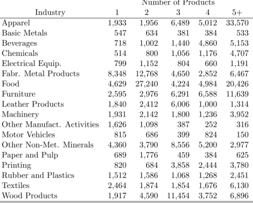
For estimation, we select two-digit sectors with at least 30 observations every year. Tables 2 and 3 report the resulting sample of eighteen sectors at two-digit classi…ca-tion codes (NACE). Products are de…ned at a nine-digit level, each one correspond-ing to an industrial product. Further details on data construction are contained in Appendix A.2.

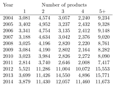
On average, 12 per cent of the sample corresponds to single-product …rms. Fur-thermore, nearly one third of the sampled …rms produces only one or two products and the median …rm produces up to three products. About one third of the sampled …rms produces …ve or more products.

Table 2: Sample size by year.

Year Number of products

1 2 3 4 5+ 2004 3,081 4,574 3,057 2,240 9,234 2005 3,402 4,952 3,237 2,432 9,328 2006 3,341 4,754 3,135 2,412 9,148 2007 3,188 4,634 3,042 2,376 9,020 2008 3,025 4,196 2,820 2,220 8,761 2009 3,084 4,190 2,802 2,164 8,282 2010 3,023 3,984 2,826 2,272 8,090 2011 2,814 3,740 2,646 2,008 7,417 2012 5,521 11,286 11,004 10,072 15,553 2013 3,699 11,426 14,550 4,896 15,771 2014 3,879 11,430 12,057 11,460 11,673

Notes: Number of observations (…rms) by year and number of products produced.

Source: IAPI.

Multi production is heterogenous across sectors. Almost half of the …rms in the Other Manufacturing Activities sector are single-product and three quarters of them produce one or two products. Manufacture of motor vehicles, fabricated metals, basic metals, food, and paper pulp also exhibit a large concentration of …rms that produce either one or two goods. On the other hand, the median …rm in the manufacture of apparel and chemicals sectors produce …ve or more products.

6.2

Production function

Table 4 contains a summary of the estimation results for Equation 16. For the translog speci…cation the estimated elasticities (dFm

t , c

F`

t , and c Fk

t ) are not

con-stant, so we report their average and standard deviation (s.d.)20. The complete set of parameter estimates and standard errors are reported in Tables A.5 and A.6 in the Appendix. The main concern with the translog speci…cation is the unrestricted production elasticities which sometimes produce negative point estimates. Thus, we also report the estimates using a Cobb-Douglas production function (i.e.

im-20_{Note that the standard deviation is not to be confused with the standard error of the}

Table 3: Sample size by sector. Number of Products Industry 1 2 3 4 5+ Apparel 1,933 1,956 6,489 5,012 33,570 Basic Metals 547 634 381 384 533 Beverages 718 1,002 1,440 4,860 5,153 Chemicals 514 800 1,056 1,176 4,707 Electrical Equip. 799 1,152 804 660 1,191

Fabr. Metal Products 8,348 12,768 4,650 2,852 6,467

Food 4,629 27,240 4,224 4,984 20,426

Furniture 2,595 2,976 6,291 6,588 11,639

Leather Products 1,840 2,412 6,006 1,000 1,314

Machinery 1,931 2,142 1,800 1,236 3,952

Other Manufact. Activities 1,626 1,098 387 252 316

Motor Vehicles 815 686 399 824 150

Other Non-Met. Minerals 4,360 3,790 8,556 5,200 2,977

Paper and Pulp 689 1,776 459 384 625

Printing 820 684 3,858 2,444 3,780

Rubber and Plastics 1,512 1,586 1,068 1,268 2,451

Textiles 2,464 1,874 1,854 1,676 6,130

Wood Products 1,917 4,590 11,454 3,752 6,896

Notes: Number of product-year observations by sector, and number of products produced. Source: IAPI.

posing x1x2 = 0 for x1; x2 2 fk; `; mg) and evaluate the sensitivity of our results

to the speci…cation.

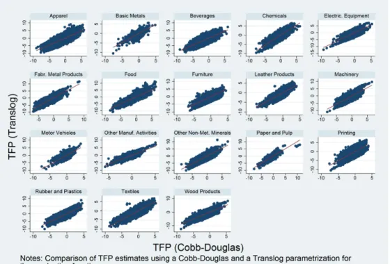
We conclude the following. First, with the exception of Other Manufacturing Activities (sector 32), the remaining sectors exhibit returns to scale (RtS) that are close to constant. Second, capital elasticities tend to be smaller than labor elasticities (beverages and apparel are the exceptions), while materials elasticities are usually the largest. Third, the Cobb-Douglas speci…cation appears to provide a good approximation. The two speci…cations not only produce similar elasticities, average in the case of the translog and constant ones in the case of the Cobb-Douglas, but also produce very similar estimates for TFP - see Figures A.1 and A.2 in the Appendix.

T a b le 4 : G M M es ti m a te s fo r th e p ro d u ct io n fu n ct io n in E q u a ti o n 1 6 b y se ct o r. S e c to r T ra n sl o g e la st ic it ie s C o b b -D o u g la s e la st ic it ie s M a te ri a ls L a b o r C a p it a l R tS M a te ri a ls L a b o r C a p it a l R tS M e a n s. d . M e a n s. d . M e a n s. d . M e a n s. d . 1 0 F o o d 0 .5 1 0 .1 0 0 .1 7 0 .0 5 0 .1 4 0 .0 8 0 .8 2 0 .0 2 0 .7 0 0 .1 7 0 .1 1 0 .9 8 1 1 B e v e ra g e s 0 .5 6 0 .1 6 0 .1 3 0 .1 2 0 .4 3 0 .1 2 1 .1 1 0 .2 7 0 .3 0 0 .1 0 0 .3 2 0 .7 2 1 3 T e x ti le s 0 .7 2 0 .2 0 0 .2 2 0 .0 8 0 .1 1 0 .1 2 1 .0 4 0 .0 7 0 .4 8 0 .3 1 0 .0 8 0 .8 7 1 4 A p p a re l 0 .6 1 0 .1 6 0 .1 2 0 .1 9 0 .3 0 0 .1 2 1 .0 3 0 .1 1 0 .4 5 0 .2 9 0 .3 1 1 .0 5 1 5 L e a th e r P ro d u c ts 0 .7 2 0 .2 1 0 .2 8 0 .1 5 0 .0 3 0 .0 3 1 .0 3 0 .0 4 0 .7 7 0 .1 4 0 .0 4 0 .9 6 1 6 W o o d P ro d u c ts 0 .7 8 0 .1 7 0 .2 3 0 .1 1 0 .0 8 0 .1 0 1 .1 0 0 .0 5 0 .6 5 0 .2 6 0 .1 1 1 .0 2 1 7 P a p e r a n d P u lp 0 .6 8 0 .0 8 0 .1 6 0 .0 8 0 .0 7 0 .0 6 0 .9 1 0 .0 7 0 .7 9 0 .1 1 0 .0 5 0 .9 5 1 8 P ri n ti n g 0 .8 0 0 .2 3 0 .2 0 0 .1 3 0 .1 3 0 .2 1 1 .1 4 0 .0 9 0 .5 6 0 .2 4 0 .2 5 1 .0 4 2 0 C h e m ic a ls 0 .7 4 0 .1 8 0 .2 3 0 .1 0 -0 .0 6 0 .0 9 0 .9 1 0 .0 8 0 .3 1 0 .4 8 0 .1 3 0 .9 2 2 2 R u b b e r a n d P la st ic s 0 .6 3 0 .0 5 0 .2 8 0 .0 6 0 .1 1 0 .0 5 1 .0 2 0 .0 4 0 .6 4 0 .2 4 0 .1 1 0 .9 9 2 3 O th e r N o n -M e t. M in e ra ls 0 .6 2 0 .1 6 0 .3 2 0 .1 9 0 .1 2 0 .0 8 1 .0 6 0 .1 2 0 .6 5 0 .2 7 0 .0 8 1 .0 0 2 4 B a si c M e ta ls 0 .5 7 0 .2 7 0 .2 6 0 .1 4 0 .1 6 0 .2 2 0 .9 9 0 .1 1 0 .5 5 0 .2 0 0 .1 1 0 .8 6 2 5 F a b r. M e ta l P ro d u c ts 0 .6 9 0 .0 6 0 .2 4 0 .0 9 0 .0 4 0 .0 5 0 .9 7 0 .0 3 0 .7 2 0 .2 0 0 .0 4 0 .9 6 2 7 E le tr ic . E q u ip m e n t 0 .7 0 0 .0 7 0 .2 3 0 .1 6 0 .0 5 0 .0 7 0 .9 7 0 .0 8 0 .7 3 0 .2 5 0 .0 2 1 .0 0 2 8 M a ch in e ry 0 .7 3 0 .0 9 0 .2 2 0 .1 4 0 .0 7 0 .0 8 1 .0 2 0 .0 2 0 .7 2 0 .2 2 0 .0 5 0 .9 9 2 9 M o to r V e h ic le s 0 .6 2 0 .2 0 0 .1 4 0 .0 6 0 .1 4 0 .1 5 0 .9 0 0 .0 9 0 .7 7 0 .0 4 0 .0 8 0 .8 8 3 1 F u rn it u re 0 .6 1 0 .2 2 0 .4 1 0 .3 5 0 .0 7 0 .0 8 1 .0 9 0 .1 1 0 .7 5 0 .2 5 0 .0 4 1 .0 4 3 2 O th e r M a n u f. A c ti v it ie s 0 .4 5 0 .0 5 0 .2 2 0 .0 4 0 .0 3 0 .0 3 0 .7 1 0 .0 2 0 .3 8 0 .2 8 0 .0 3 0 .6 9 N o te s: M e a n a n d st a n d a rd d e v ia ti o n (s .d .) o f th e e st im a te d tr a n sl o g e la st ic it ie s. C o b b -D o u g la s sp e c i… c a ti o n a ls o re p o rt e d fo r c o m p a ri so n . E st im a ti o n m e th o d : G M M . In st ru m e n t se t: c u rr e n t le v e ls o f la b o r a n d c a p it a l (t h e ir sq u a re s a n d p ro d u c t) ; la g g e d le v e ls o f c a p it a l, la b o r, m a te ri a ls , p ri c e s, a n d in d u st ry p ri c e s (t h e ir sq u a re s a n d p ro d u c ts ), re a l G D P , u n it -p ro d u c t d u m m ie s, a n d th e p ro b a b il it y o f re m a in in g si n g le -p ro d u c t. T h e p ro b a b il it y o f re m a in in g si n g le p ro d u c t is a n e st im a te d P ro b it o n p ro d u c t a n d in d u st ry p ri c e s, re a l G D P a n d a ll in p u ts (t h e ir sq u a re s a n d p ro d u c ts ). R tS is su m o f th e in p u t e la st ic it ie s: a v a lu e la rg e r/ e q u a l/ sm a ll e r th a n o n e in d ic a te s in c re a si n g / c o n st a n t/ d e c re a si n g re tu rn s to sc a le .

6.3

The demand function

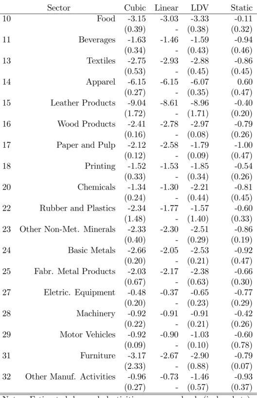
Figure 3 plots the estimated demand curves for the nested-homothetic speci…ca-tion in Equaspeci…ca-tion 9 and Table 5 contains the estimated own-price elasticities ( qp_).

Because the log-cubic approximation for function d ( ) produces varying own-price elasticities, we report their mean and standard deviation in Table 5, while a log-linear speci…cation is also reported for robustness. Tables A.7 and A.8 in the Appendix document the full set of estimated coe¢ cients and signi…cance levels for the log-cubic and log-linear speci…cations, respectively. Average own-price elas-ticities are estimated in the range -1 to -4 and are similar in the linear and the cubic case. There is also little evidence of non-constant elasticities, as suggested by Figure 3. -20 0 20 40 -30 -20 -10 0 10 -10 -5 0 5 -10 0 10 20 -10 -5 0 5 -15 -10 -5 0 5 -20 -10 0 10 -100 -50 0 50 -100 -50 0 50 100 0 10 20 30 40 -5 0 5 10 -10 -5 0 5 -20 -10 0 10 -20 -10 0 10 -10 0 10 20 0 20 40 60 -10 0 10 20 30 -30 -20 -10 0 10 -4 -2 0 2 4 -5 0 5 -4 -2 0 2 -5 0 5 -5 0 5 -5 0 5 -5 0 5 -4 -2 0 2 4 -4 -2 0 2 4 -5 0 5 10 -5 0 5 -5 0 5 -5 0 5 -4 -2 0 2 4 -5 0 5 -5 0 5 -5 0 5 -5 0 5 10

Apparel Basic Metals Beverages Chemicals Electric. Equipment

Fabr. Metal Products Food Furniture Leather Products Machinery

Motor Vehicles Other Manuf. Activities Other Non-Met. Minerals Paper and Pulp Printing

Rubber and Plastics Textiles Wood Products

Predicted ln(q

ijt

)

ln(pijt)

Notes: Predicted demand (over own price) and 95% confidence intervals for the cubic parametrization. Holding income, industry and aggregate prices constant.

Figure 3: Estimated demand functions bysector

To further evaluate the robustness of our estimates, we also estimate a simple static model, assuming that the demand level is serially uncorrelated over time,

Table 5: Estimated demand own-price elasticities ( qp ₎

Sector Cubic Linear LDV Static 10 Food -3.15 -3.03 -3.33 -0.11 (0.39) - (0.38) (0.32) 11 Beverages -1.63 -1.46 -1.59 -0.94 (0.34) - (0.43) (0.46) 13 Textiles -2.75 -2.93 -2.88 -0.86 (0.53) - (0.45) (0.45) 14 Apparel -6.15 -6.15 -6.07 0.60 (0.27) - (0.35) (0.47) 15 Leather Products -9.04 -8.61 -8.96 -0.40 (1.72) - (1.71) (0.20) 16 Wood Products -2.41 -2.78 -2.97 -0.79 (0.16) - (0.08) (0.26) 17 Paper and Pulp -2.12 -2.58 -1.79 -1.00 (0.12) - (0.09) (0.47) 18 Printing -1.52 -1.53 -1.85 -0.54 (0.33) - (0.34) (0.26) 20 Chemicals -1.34 -1.30 -2.21 -0.81 (0.24) - (0.44) (0.45) 22 Rubber and Plastics -2.34 -1.77 -1.57 -0.60 (1.48) - (1.40) (0.33) 23 Other Non-Met. Minerals -2.33 -2.30 -2.51 -0.86 (0.40) - (0.29) (0.19) 24 Basic Metals -2.66 -2.05 -2.53 -0.92 (0.20) - (0.21) (0.47) 25 Fabr. Metal Products -2.03 -2.17 -2.38 -0.66 (0.67) - (0.63) (0.30) 27 Eletric. Equipment -0.48 -0.37 -0.65 -0.77 (0.20) - (0.23) (0.29) 28 Machinery -0.92 -0.91 -0.91 -0.42 (0.22) - (0.21) (0.26) 29 Motor Vehicles -0.92 -0.90 -1.03 -0.60 (0.09) - (0.10) (0.78) 31 Furniture -3.17 -2.67 -2.90 -0.79 (2.33) - (0.88) (0.07) 32 Other Manuf. Activities -0.96 -0.73 -1.46 -0.93 (0.27) - (0.57) (0.37) Notes: Estimated demand elasticities: mean and s.d. (in brackets). Cubic, linear, LDV, and static speci…cations. LDV allows for persistence in addition to serial dependence.

i.e. ( t 1) = 0. Additionally, we consider a more general model, where besides

the serially correlated (Markov) demand level ( ) we also allow for separate e¤ects from the lagged dependent variable (LDV), i.e. true dependence. The results are displayed in the last two columns of Table 5. First, adding true dependence does not produce substantial changes to the estimated elasticities. This is due to the fact that the estimated e¤ects from the LDV are small in magnitude. Second, the static model produces small own-price elasticities, in most cases smaller than one. This is due to the existence of strong observed persistence (serial correlation) in the demand level. By ignoring this persistence, we under-estimate price sensitivity due to the fact that a given price change will produce a much smaller response of sales, as most of sales are somehow pre-determined by the serially correlated demand level. In a static setting, it thus seems that sales are irresponsive to prices, where this irresponsive nature is due to the dynamic (persistent) element.

6.4

Markup measures and distribution

Having estimated the production function we can go back to our measure of markups in Equation 6. Then, using the observable shares, we can assess the relative performance of markup measures using materials and labor. If both labor and materials are fully ‡exible, the following equality holds:

t= Fm t sm t = F` t s` t :

Thus, we would expect markups in Figure A.5 to sit on the 45o line (or on some other line passing through the origin, in case the estimated elasticities were biased). We actually observe a negative relationship, suggesting some form of departure from equality. One of the several cases that can generate this departure is the existence of a labor wedge, as found in recent literature - see Bils et al. (2018).

Using materials for measuring markups properly, we …nd that they exhibit a substantial heterogeneity in the product-…rm-year space in all eighteen industries considered. Figure A.3 in the Appendix, reports markup distributions using both our baseline translog speci…cation with varying elasticities and constant elasticities from the Cobb-Douglas speci…cation. In general, distributions are skewed to the

right with many small markups and a heavy tail of large markups21_.

Figure A.4, also in the Appendix, reports the distribution of markups for single-product …rms, for which the left tail disappears. This is particularly noticeable in sectors such as leather, basic metals, food or furniture, that actually exhibit multi-peaked distributions for all product-…rm-year observations with the …rst peak vanishing once we only consider single-product …rms.

7

Markups

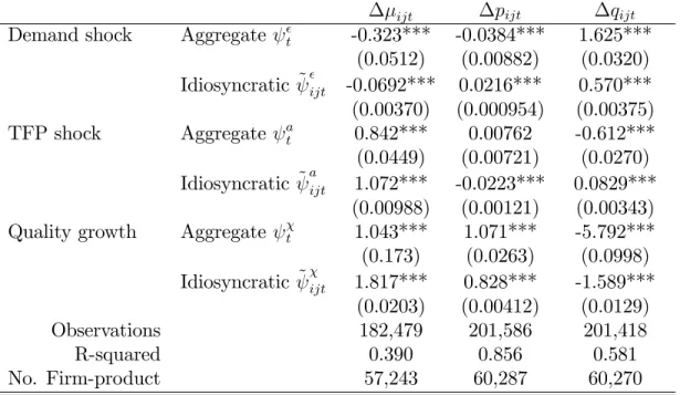
In this section we gather the main results of the article. We show that markups are pro-cyclical with TFP and counter-cyclical with demand shocks, and we also demonstrate that this result is robust to both the presence of multi-production and to alternative demand function speci…cations. Finally, we go back to the decomposition in section 4 and disaggregate TFP and demand shocks into price vs. quantity and aggregate vs. idiosyncratic e¤ects.

7.1

The cyclical behavior of markups

In Table 6, we evaluate the response of markups, prices, and sales to the TFP ( a) and demand ( ) shocks estimated in the previous section. To control for potential biases, we also include …rm-product …xed e¤ects as well as input-quality shock ( ) in the regressions. Overall, markups exhibit a positive response to supply shocks and a negative response to demand shocks. Changes in quality are also positively correlated with markups.

We can quantify the responses: a 10 per cent demand shock is predicted to increase prices by 0.2 per cent and sales by 5.7 per cent, while decreasing markups by 0.6 percentage points; a positive 10 per cent TFP shock is predicted to reduce prices by 0.2 per cent and to increase sales by 0.9 per cent, while increasing markups by 10.6 percentage points. In a nutshell, a positive TFP shock passes through as slightly lower prices, with the companies retaining the lower cost as a larger markup. On the other hand, a positive demand shock leads to a modest increase in prices and a reasonable expansion in sales; however, short-run production restrictions lead

21_{Very small markups (less than 1) are either explained by multi-product …rms setting small}

to an increase in marginal costs, which explains the observed decrease in markups. Overall, both demand and TFP shocks lead mostly to a response in sales, with prices remaining relatively irresponsive. Table A.9 in the Appendix shows that the e¤ects are robust across sectors, with the exceptions being the printing and the furniture sectors, for which markups exhibit no statistically signi…cant cyclicality.

The results can be interpreted in light of the analysis in section 4. First, prices increase with demand shocks and decrease with supply shocks. This is consistent with having PqQ + P > 0 and PqQa < 0. The second result is as expected,

with a positive supply shock moving prices downward along the demand curve. However, a demand shock would have a priori an ambiguous e¤ect, as it exhibits a positive direct e¤ect on prices, but a negative indirect e¤ect by increasing output (there is an upward shift in the demand schedule and downward slide caused by the expansion in quantity). Our result implies that the direct e¤ect dominates.

Second, quantities sold (sales) are positively correlated with both supply and demand shocks, and are consistent with Q > 0 and Qa < 0. Again, this is expected

with standard slopes for the two above-mentioned curves.

As we can see, markups increase with supply shocks and decrease with demand shocks, consistent with a > 0 and < 0. An increase in TFP pushes marginal

costs down (Ca < 0) and this translates into a lower price. Results suggest that

part of the lower marginal cost is absorbed by the company as a larger markup, at least in the short run22. Referring to Equation 2, the positive direct e¤ect of a supply shock (Ma > 0) dominates the negative indirect e¤ect (MqQa < 0).

Finally, a shift in demand is associated with an increase in both prices and sales. As sales increase, so do marginal costs. The results suggest that the increase in marginal costs is stronger than the increase in prices, implying that the indirect e¤ect (MqQ < 0) dominates the direct e¤ect (M > 0) in Equation 3.

Summing up, the results are consistent with relatively large values of Q and Ca

and relatively small values of P . Before presenting the quantitative decomposition of these e¤ects in section 7.3, we …rst provide a series of robustness checks.

T a b le 6 : R es p o n se to sh o ck s M o d el : C u b ic L in ea r ij t ln pij t ln qij t ij t ln pij t ln qij t T F P 1 .0 6 4 * * * -0 .0 2 2 9 * * * 0 .0 9 1 9 * * * 1 .0 5 9 * * * -0 .0 2 3 5 * * * 0 .0 9 0 1 * * * sh o ck (0 .0 0 9 2 1 ) (0 .0 0 1 2 8 ) (0 .0 0 3 6 5 ) (0 .0 0 9 1 6 ) (0 .0 0 1 3 1 ) (0 .0 0 3 5 7 ) D em a n d -0 .0 6 4 5 * * * 0 .0 1 8 7 * * * 0 .5 7 3 * * * -0 .0 7 0 0 * * * 0 .0 1 8 3 * * * 0 .5 8 4 * * * sh o ck (0 .0 0 3 5 4 ) (0 .0 0 0 9 4 4 ) (0 .0 0 3 7 1 ) (0 .0 0 3 5 2 ) (0 .0 0 0 9 1 8 ) (0 .0 0 3 5 8 ) Q u a li ty 1 .7 7 7 * * * 0 .8 3 8 * * * -1 .5 9 4 * * * 1 .7 6 9 * * * 0 .8 4 6 * * * -1 .5 1 0 * * * sh o ck (0 .0 1 9 1 ) (0 .0 0 4 2 3 ) (0 .0 1 2 7 ) (0 .0 1 8 5 ) (0 .0 0 4 0 4 ) (0 .0 1 2 1 ) O b se rv a ti o n s 1 8 3 ,3 9 3 2 0 2 ,7 9 0 2 0 2 ,0 0 6 1 8 4 ,0 6 2 2 0 3 ,6 6 3 2 0 2 ,8 8 6 R 2 0 .3 8 9 0 .8 5 9 0 .5 8 7 0 .3 8 9 0 .8 5 7 0 .5 9 9 N o . o f … rm -p ro d . 5 7 ,3 7 0 6 0 ,4 4 7 6 0 ,3 4 9 5 7 ,4 6 0 6 0 ,5 4 6 6 0 ,4 4 9 M o d el : L D V S ta ti c ij t ln pij t ln qij t ij t ln pij t ln qij t T F P 1 .0 9 0 * * * -0 .0 2 0 7 * * * 0 .0 7 9 6 * * * 1 .0 5 8 * * * -0 .0 1 8 3 * * * 0 .0 1 2 4 * * * sh o ck (0 .0 0 9 5 1 ) (0 .0 0 1 2 8 ) (0 .0 0 3 6 4 ) (0 .0 0 8 7 5 ) (0 .0 0 1 2 3 ) (0 .0 0 1 1 3 ) D em a n d -0 .0 7 8 9 * * * 0 .0 1 5 5 * * * 0 .5 6 1 * * * -0 .1 6 7 * * * -0 .0 1 8 7 * * * 0 .9 7 2 * * * sh o ck (0 .0 0 3 6 8 ) (0 .0 0 0 9 5 0 ) (0 .0 0 3 5 8 ) (0 .0 0 4 0 7 ) (0 .0 0 0 9 5 0 ) (0 .0 0 0 8 7 4 ) Q u a li ty 1 .9 1 7 * * * 0 .8 6 4 * * * -1 .7 3 2 * * * 1 .6 6 4 * * * 0 .8 7 7 * * * -1 .0 5 8 * * * sh o ck (0 .0 2 1 1 ) (0 .0 0 4 4 9 ) (0 .0 1 3 2 ) (0 .0 1 4 8 ) (0 .0 0 3 0 5 ) (0 .0 0 3 1 2 ) O b se rv a ti o n s 1 8 0 ,8 8 2 1 9 9 ,9 4 3 1 9 9 ,1 0 8 1 8 6 ,9 0 1 2 0 6 ,9 7 4 2 0 6 ,5 4 1 R 2 0 .3 9 5 0 .8 5 5 0 .5 8 5 0 .3 9 6 0 .8 6 5 0 .9 5 9 N o . o f … rm -p ro d . 5 7 ,1 3 0 6 0 ,1 8 1 6 0 ,0 6 0 5 7 ,8 1 5 6 0 ,9 5 7 6 0 ,9 1 3 N o te s: R eg re ss io n re su lt s w it h … x ed … rm -p ro d u ct e¤ ec ts . C lu st er ed st d . er ro rs in b ra ck et s. C u b ic , li n ea r, L D V , a n d st a ti c sp ec i… ca ti o n s. L D V a ll o w s fo r p er si st en ce in a d d it io n to se ri a l d ep en d en ce . S ig n i… ca n ce : * * * 1 % , * * 5 % a n d * 1 0 % .

7.2

Robustness checks

7.2.1 Alternative demand speci…cations

The qualitative results in the previous section are robust to a series of di¤erent speci…cations for the demand function. In Table 5, we reported how estimated elasticities varied in four di¤erent models: (i) cubic approximation (baseline), (ii) linear approximation, (iii) LDV (true dependence), and (iv) static demand. In Table 6 we display the response of markups, prices, and quantities to the demand shocks, estimated with the four di¤erent speci…cations. Overall, the numbers are very similar in the cubic, linear, and true-dependence cases, with the markup coe¢ cient hovering between 1:05 and 1:09 for TFP shocks and between 0:065 and 0:079for demand shocks.

However, a signi…cant di¤erence emerges if we use a static demand model. In this case, markup responses are much stronger, increasing to 0:17 for demand shocks, thus becoming more counter-cyclical with demand shocks. Price and sales response coe¢ cients are also larger, becoming negative for prices. The stronger cyclicality of markups is due to the misspeci…cation of the demand shock. In the static setting, we have seen that estimated demand curves are inelastic. This means that we obtain much smaller quantity responses to price changes and we underestimate demand shocks. For instance, the standard deviation of demand shocks is 1:14 in our baseline case and 0:70 in the static case. The smaller volatility of demand shocks in the static case, results in overestimating their e¤ect on the markups.

7.2.2 Does the number of products matter?

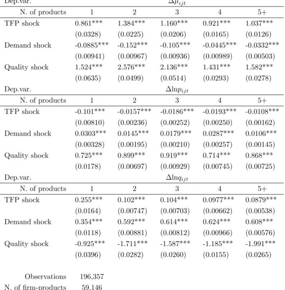
The qualitative results in the previous subsection refer to averages across single- and multi-product …rms. Table 7 contains the results obtained from splitting the sample by the number of products. By comparing it with Table 6, we readily observe that, although the qualitative responses of markups, prices, and quantities do not change, both for TFP and demand shocks, there is a substantial heterogeneity in the estimates: the markup coe¢ cients estimates for single-product …rms are 0:86 for TFP and 0:09 for demand shocks and they are 1:04 and 0:03 for …rms producing 5 of more goods. The e¤ects on markups are stronger for single-product

…rms and become weaker as …rms produce more products. The e¤ects on prices and quantities depend on the origin of the shocks: for TFP shocks, multi-product …rms increase sales and reduce prices by less; for demand shocks, multi-product …rms increase prices by less and sales by more. Consequently, markups tend to be more counter-cyclical with demand shocks for …rms producing one or two goods and they are less counter-cyclical for …rms that produce …ve or more goods. Furthermore, markups seem to become more pro-cyclical with TFP shocks for multi-product …rms, but this pattern is much less clear and the discrepancy is not as large as in the demand shock.

Finally, Table A.10 in the Appendix shows that the heterogeneity remains when we control for size, measured as the logarithm of employment. Thus, reduced cyclicality in the response to shocks for multi-product …rms is not purely driven by size (economies of scale), as economies of scope explain part of the …rms’response to shocks.23 _{Since both prices and quantities react similarly for single- and}

product …rms, the less responsive markups points to a larger ‡exibility from multi-product …rms on the marginal-cost side, suggesting that multi-multi-product …rms can adjust production by reallocating productive capacity across goods24_{, rather than}

changing its market power.

7.2.3 Labor-based markup and revenue-based TFP shocks

One question remains. How important are the corrections? In order to answer this, we compare our results to those obtained by using a revenue–based measure of TFP or by using a labor-based markup measure, as commonly found in the literature.

First, we start by using the alternative revenue-based TFP (TFPy) to obtain the TFP shocks. We use the estimated coe¢ cients from the Cobb-Douglas pro-duction function reported in Table 4 and construct TFPy using revenues instead of quantity. This way we only change one element, the use of revenues to calculate TFP, while we hold …xed the potential di¤erences originated by di¤erent production function elasticities. As reported in Table 8, when we use revenues instead of

quan-23_{Hong (2017) reports size-related heterogeneity in unconditional cyclicality of markups with}

respect to GDP.