Detecting city-hinterland pairs with a community detection algorithm

DETECTING CITY-HINTERLAND PAIRS WITH A

COMMUNITY DETECTION ALGORITHM

II

Detecting City-Hinterland Pairs With a Community

Detection Algorithm

Dissertation supervised by

Prof. Dr. Judith Verstegen

Institute for Geoinformatics

Westfälische Wilhelms-Universität, Münster, Germany

Co-supervised by

Prof. Dr. Brian Dermody

Prof. Dr. Roberto Henriques

NOVA Information Management School University of New Lisbon, Lisbon, Portugal

III

Declaration

I hereby certify that this thesis, entitled “Detecting City-Hinterland Pairs with a Community Detection Algorithm”, has been entirely composed by me and is based on my own work and under the guidance of my supervisors. No other person’s work has been used without due acknowledgment. All the references used have been cited, and all sources of information, including graphs, illustrations and data sets, have been specifically acknowledged.

Signature:

……… Münster, February 2019

IV

Acknowledgments

I would like to express my sincere gratitude to my supervisor Dr. Judith Verstegen,for continuous

support on my research, for her patience, enthusiasm, guidance and motivation throughout the work. I would like to express my heartfelt gratitude to my co-supervisor, Dr. Brian Dermody for his ideas, suggestions, and comments that were really helpful for completing this work. I am also thankful to Dr. Roberto Henriques for co-supervising my thesis. I will always be in debt to their guidance.

I am grateful to the Erasmus Mundus program for providing me the opportunity and fellowship to pursue the Master's degree in Geospatial Technologies. It was really a wonderful opportunity to learn in a multi-cultural environment with my amicable classmates taught by inspirational teachers. I am grateful to all those who have played a part in institutionalizing this course. I sincerely applaud the efforts of this hardworking team from all three partner universities of this master's program.

Finally, I would like to take this opportunity to express my love and gratitude to my family who has always been by my side, encouraging and supporting me throughout the time period of my study. My all endeavors are the trust of my parents, the encouragement of my sisters and brothers.

V

Detecting City-Hinterland Pairs With a Community

Detection Algorithm

Abstract

With the increasing urbanization, cities tend to grow together with the infrastructure networks beyond their administrative boundaries. Identifying the right dimension of the city is thus challenging for the geographers. One way to represent a city could be identifying the city core and its hinterland as a part of the city itself. Since the transport network is used to deliver the resources between the city and its hinterland, we can hypothesize that the connectedness between the city and its hinterland is represented by the transport network topology. Hence, it would be justifiable to consider the transport network topology as a foundation for identifying hinterlands. One way to achieve this task of identifying hinterland utilizing the transport network topology is by using community detection algorithms. This thesis presents and evaluates a methodology for defining city-hinterland pairs at a regional level using community detection algorithms applied to the transport network. Easily accessible OpenStreetMap(OSM) road network data was used as the data for our research. We used three modularity optimization based community detection algorithms to identify communities in the road network. The identified communities were assigned to city core areas and hinterland based on the proposed criteria. Results from different algorithms were compared among each other and with the OECD Functional Urban Areas(FUAs). Similarity among the results between the three algorithms was acceptable with the average Goodness-of-fit (GOF) scores of 0.60 and 0.65 for core urban area and hinterland respectively. With OECD FUAs results showed less similarity with average GOF scores of 0.40 and 0.31 for core urban area and hinterland respectively. The disimilarity of our result with OECD data is justifiable as the OECD FUAs use population data and commuting data of administrative units without considering transport connectivity but we use only road network as the basis for identifying city and hinterland communities.

Keywords: City; Hinterland; Transport Network; Community Detection Algorithms;

VI

Acronyms

OECD Organisation for Economic Co-operation and Development FUAs Functional Urban Areas

GIS Geographic Information System OSM OpenStreetMap

VII

Table of Contents

Acknowledgments ... IV Abstract ... V Acronyms ... VI Table of Contents ... VII List of Figures ... IX List of Tables ... X 1. Introduction ... 1 1.1. Background ... 1 1.2. Research Gap... 2 1.3. Research Questions ... 3 1.4. Research Objectives ... 4 2. Theoretical Background... 5

2.1. Community Detection Algorithms ... 5

2.2. Modularity Optimization Algorithms ... 5

2.2.1. Louvain Algorithm ... 6 2.2.2. Leiden Algorithm ... 7 2.2.3. Fastgreedy Algorithm ... 8 3. Methodology ... 9 3.1. Study Area ... 9 3.2. Datasets Used ... 10 3.3. Data preprocessing ... 11

3.4. Implementation of Community Detection Algorithms ... 14

3.4.1. Louvain Algorithm ... 14

3.4.2. Leiden Algorithm ... 15

3.4.3. Fastgreedy Algorithm ... 16

3.4.4. Post-processing of results ... 16

3.4.5. Delineation of community areas ... 16

VIII

3.4.7. Assigning city names ... 18

3.4.8. Identifying Hinterlands ... 18

3.4.9. Comparing Results ... 19

4. Results and Discussion ... 21

4.1. Communities detected on the weighted and non-weighted road network ... 21

4.2. Classification of city core urban areas and hinterland ... 23

4.3. Comparing the results... 26

4.4. Resolution limit in Algorithms ... 29

4.5. Limitations of our work... 30

5. Conclusion and future works... 32

5.1. Conclusion ... 32

5.2. Future works ... 34

Bibliography ... 35

IX

List of Figures

Figure 1: Louvain algorithm steps. Reprinted figure from [28] ... 7 Figure 2: An example showing disconnected community. a) Initial partition b) Internally

disconnected community (in red color) after moving of crucial node 0. Reprinted figure from [29] ... 8 Figure 3: Study area: Three government regions ((Regierungsbezirke) in North

Rhine-Westphalia, Germany ... 9 Figure 4: Data preprocessing steps for creating clean and simplified road network data ... 11 Figure 5: Small section of the road network data used a) Downloaded road network data b) Road network data after performing preprocessing steps ... 14 Figure 6: Steps for converting partition nodes into community areas ... 17 Figure 7: Goodness-of-Fit score calculation between two intersecting polygons (Adapted from Hargrove et. al [36]) ... 19 Figure 8: Communities detected on the unweighted and weighted road network by different algorithms a)LouvainNonWgt b)LouvainWgt c)LeidenNonWeight d)LeidenWgt

e)FastgreedyNonWgt f)FastgreedyWgt ... 22 Figure 9: Core communities classified using natural breaks classification for different algorithms a)LouvainWgt b)LeidenWgt c)FastgreedyWgt d)LouvainLev3Wgt e)LouvainLev2Wgt ... 24 Figure 10: City core areas and hinterland identified by three algorithms a) LouvainWgt b) LeidenWgt c)FastgreedyWgt ... 25 Figure 11: Goodness-of-fit scores of core areas identified by three algorithms with OECD core urban areas ... 27 Figure 12:Goodness-of-fit scores of hinterland areas identified by three algorithms with OECD hinterlands ... 28 Figure 13: Communities based on input road network a)&b) LouvainWgt c)&d)LeidenWgt e)&f) FastgreedyWgt ... 30

X

List of Tables

Table 1: Abbreviations used for different algorithm' s results ... 20

Table 2: Modularity values and number of communities detected across different algorithms for the unweighted and weighted road network... 21

Table 3: Intersection density break values used for classification of core communities ... 23

1

1. Introduction

1.1.Background

More than 55% of the world's population is currently residing in urban areas and this percentage is expected to rise up to 68% by 2050 [1]. With the increasing urbanization, cities tend to grow beyond the administrative boundaries defined with the result that these boundaries no longer depict the real world scenario of the city's urban structure [2]. This leaves behind a new point of discussion on how can a city boundary be identified that portrays a better representation than the administrative boundary. One way to address this problem could be identifying the city and its hinterland as a part of the city itself that can capture the socio-economic interactions between the city and it's surrounding.

The term 'hinterland' might refer to the area which originates immediately beyond the core area of a city together with infrastructural networks or might be the distant area either regional, national or global defined by the products consumed within the city [3]. This research will focus on the former type of hinterland, which is also recognized as a functional region or urban hinterland. In summary, every city is comprised of a core urban area and its adjoining hinterland which is

economically tied with that particular city [4].In return, cities which hold a large proportion of the

population have to depend on their hinterland for their supply of resources such as water, agricultural products, etc. [5].

The importance of identifying hinterland of any city has long been recognized by many authors for the sake of modeling relationships and interdependencies between city and hinterland [5, 6, 7] . For the sustainable development of a city, it is important that the city planners work on the policy integration and development of its associated hinterland as well [8, 9] . Thus it is crucial to identify these city- hinterland pairs so that we can better understand the underlying relationships between

them for better sustainability. In this context, the OECD and the European Commission have

jointly developed a new definition of a city and its commuting zone (hinterland) under the name of Functional Urban Areas (FUAs) [10].

The paramount prerequisite for being a hinterland is the access via transportation network which is used to deliver resources between a city and its hinterland [6]. Thus, we can hypothesize that the transport network topology represents the connectedness between a city and its hinterland more

2

effectively than any other infrastructural networks. The transport network is a type of spatial network that is composed of nodes (vertices) and edges guided by geometry embedded in Euclidean space [11]. The spatial arrangement of these nodes and edges together with the other factors such as distance and travel time can be utilized for discovering some patterns exhibited by the road networks. One of these patterns could be the city – hinterland pairs as communities (modules or clusters) in this network. In general, a community can be characterized as a special property exhibited by the networks where the nodes seem to have more dense connections within themselves and few connections with the rest of the network [12]. In the case of the transport network, these communities might correspond to each city-hinterland pair. One of the ways to detect these communities is by using community detection algorithms [13].

Fundamentally, community detection algorithms tend to group the nodes in a network into different communities such that connections between nodes within a community are denser than the connections between nodes of different communities [14]. Various community detection algorithms have been developed and implemented in different scientific fields based on their own requirements [15]. However, no particular algorithm has been developed that fits well for all types of real-world networks [16]. In order to detect communities from real-world networks, it is advisable to use several algorithms and use the results that are similar across different methods [17]. This is because of the difficulty in validating the communities detected. One of the most tractable and popular methods to detect communities is modularity optimization algorithm, which involves maximizing the quality measure for network partition called modularity [18]. For spatial networks like the transport network, a modularity optimization algorithm is a commonly used method that has been implemented for detecting communities so far. In case of spatial networks, this method of community detection was applied earlier to detect spatial housing submarkets on the street network of London [19] and a similar approach was applied to the road network of Africa to identify communities with a high burden of malaria disease [20].

1.2.Research Gap

Very few works have been done in the field of developing a harmonized methodology for the detection of city-hinterland pairs. The method developed by OECD was implemented for identifying the core urban area and the urban hinterlands of various cities in 29 OECD countries.

3

They utilized the population density data to identify urban cores and commuting data to identify urban hinterlands. Besides, few methodologies have been proposed for detecting hinterlands such as the overlay of administrative boundaries and Thiessen polygons created with city nodes [6] and

GIS-based methods (using gravity models) [21]. Also, various researches are more focused on

identifying the hinterland of a particular major city only using manual procedures [22, 23] .

Though few methodologies mentioned above have been implemented or proposed for detecting the hinterland, a harmonized methodology that can be applied to any countries to detect city-hinterland pairs is still missing. The OECD method needs the commuting data for identifying hinterlands, but these data are not available in most of the countries. Also, the administrative units they used as a base to categorize core urban and hinterland might not be appropriate. One way to solve this problem could be the use of widely available road network data to identify city- hinterland pairs.

Applying community detection algorithms in the transport network might uncover some useful pattern that can be significant for identifying city-hinterland pairs. However, no distinct methodology has been proposed till date for detecting city-hinterland pairs using both transport network topology and community detection algorithms. In summary, there is a need of research that would focus on developing a harmonized methodology utilizing the transport network topology as the main consideration (e.g. community detection algorithms) for detecting city-hinterland pairs of a state or a country as a whole. Therefore, this thesis will be focused on developing and evaluating a methodology for defining city-hinterland pairs at a regional level using community detection algorithms applied to the transport network.

1.3.Research Questions

The following research questions will be addressed for the stated problem:

i. How similar or different are the detected communities on the transport network across different community detection algorithms?

ii. To what extent do the detected city-hinterland pairs using our approach resemble with OECD Functional Urban Areas?

iii. What could be the possible reasons for the similarity or differences found on the communities detected by different algorithms and with OECD FUAs?

4 1.4.Research Objectives

In order to answer the above research questions the following objectives are to be fulfilled:

i. Explore existing community detection algorithms and identify any three of them that

can be implemented in the case of road networks.

ii. Implement community detection algorithms to detect communities on the transport

network and compare the results among different algorithms.

iii. Identify the city core urban areas and their hinterland and compare the results with

5

2. Theoretical Background

2.1.Community Detection Algorithms

In the last decade, the detection of communities in the network has been one of the widespread topics in the field of network science [16]. Generally, a community is a distinctive property exhibited by the networks where the nodes seem to have more dense connections within themselves and few connections with the rest of the network. Various community detection algorithms have been introduced by researchers such as Centrality-Based Community Detection [24], k-Clique Percolation [25], Modularity Optimization [12] and Spectral Partitioning [26] for identifying communities in the network. The main difference among these algorithms lies in the

heuristics defined to identify communities in the networks [16]. The mostwidely used algorithm

in recent practice is modularity optimization algorithm. Also, the modularity optimization algorithms have been previously implemented in the case of spatial networks and the results showed similarity with the real world community regions [19, 20]. In this research, we will adopt the methods based on modularity optimization to detect communities in the road network.

2.2.Modularity Optimization Algorithms

Modularity optimization algorithms involve maximizing the quality measure for network partition called Newman-Girvan modularity [18]. This quality measure gives the estimation about how well the communities of a network are partitioned by subtracting the density of edges connected within a module from the expected density of edges in the same network when there is no community

structure. Modularity can be calculated for both weighted and unweighted networks. For the

unweighted networks, modularity (Q) is generally defined as:

Q= (fraction of edges within communities)

–

For the weighted networks, the fraction of edges is replaced by the strength of nodes i.e. the sum of the weights of edges adjacent to the nodes.

The mathematical expression for modularity (Q) in weighted networks is:

6

Where is the weight of edge connecting nodes i and node j,

=

∑

= ∑

is a Kronecar Delta Function which equals 1 if i and j are in sthe ame community and 0 otherwise,

c

c

In equation 2, the term is the expected weight of the edge connecting node i and node j in

the null model of modularity proposed by Newman and Girvan.

One of the main limitations of modularity optimization methods is the resolution problem. Due to this, the algorithms could fail in identifying communities smaller than a certain size or weight existing in the network at optimal modularity partition [27].

2.2.1. Louvain Algorithm

The Louvain algorithm [28] is one of the most widely used modularity optimization based algorithms for identifying communities in large networks. It can be applied to both unweighted and weighted networks.

This algorithm uses two main iterative phases for detecting communities with higher modularity. At first, each node is assigned to different communities so that the number of communities is equal

to a number of nodes in the network.After then, each node is moved from the current community

to another community and the modularity is checked. If the modularity doesn't change after moving, the node stays in the same community and otherwise, the node is assigned to the community which has the highest increase in modularity. This step is repeated for each node until

there is no improvement in modularity. After completing this step, one level ofcommunities is

detected.

In the second phase, a new network is created by converting the communities in the previous phase into nodes. Then edges between these nodes are created and assigned the sum of the weight of links between corresponding communities. This process is repeated with the newly formed

7

aggregate network to detect communities at a higher level. The algorithm stops if no further improvement in the modularity of the whole partition is possible.

.

2.2.2. Leiden Algorithm

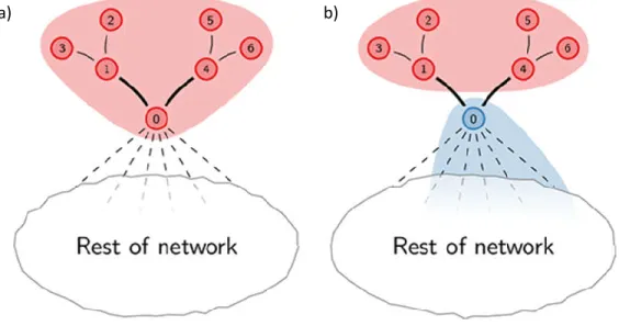
The Leiden algorithm [29] is a recently introduced modularity optimization based algorithm that can be used for both weighted and unweighted large networks. This algorithm is considered as an improvement to the Louvain algorithm discussed above because it solves some of the issues such as badly connected communities that were present in the Louvain algorithm [29]. In Louvain algorithm (Section 2.2.1), while moving the nodes from one community to another, it might move the crucial node that acts as a bridge with the rest of the communities. After moving that crucial node, the old community would be disconnected (Figure 2b). This leads to the identification of badly connected and disconnected communities in Louvain Algorithm. Leiden algorithm solves the aforementioned problem and helps in detecting improved communities in the network [29].

The Leiden algorithm also starts with the communities equal to the number of nodes. After then, the algorithm moves individual nodes from one community to another to find communities that increases modularity. The next step involves the refinement of the individual communities found

8

in the earlier step. After the refinement step, the initial community might split into multiple sub-communities ensuring well-connected sub-communities. After then, aggregation of the community nodes is done based on the refined partition. These steps are iterated until no more improvement can be made in terms of modularity value.

2.2.3. Fastgreedy Algorithm

The Fastgreedy algorithm [30] is another modularity optimization method of community detection which can also be applied in the case of large weighted and unweighted networks. In this algorithm also, the number of communities are equal to the number of nodes (n) at the beginning but the edges are not present during this stage. Insertion of the edges is done one by one and the modularity

is checked after the addition of each edge.The edge to be inserted is chosen in such a way that

such that the new partition gives the maximum increase of modularity with respect to the previous arrangement. After adding the first edge in the disconnected nodes, the number of communities decreases from n to n – 1. This will give the new partition in the network with n-1 communities. A similar procedure is followed to insert remaining edges. The change in modularity is calculated in each iteration step after merging of two communities so that we can choose which merger is the best. This process is repeated until the single community is formed. The best partition of the network into communities is chosen from this subset of partitions for which the modularity is maximum.

Figure 2: An example showing disconnected community. a) Initial partition b) Internally disconnected community (in red color) after moving of crucial node 0. Reprinted figure from [29]

9

3. Methodology

3.1.Study Area

Three of the five government regions (Regierungsbezirke) in North Rhine-Westphalia state,

Germany i.e. Münster, Düsseldorf, and Köln were chosen as the study area for our research. The study area features 12 cities with more than 200,000 population and 3 of them are from the list of Germany's 10 largest cities. Availability of OECD Functional Urban Areas data for most of the cities in this region in order to validate our result was the main reason for choosing this study area.

Figure 3: Study area: Three government regions ((Regierungsbezirke) in North Rhine-Westphalia, Germany (Data Source: www.gadm.org)

10 3.2.Datasets Used

As one of the motives of our research was to use fewer data possible which are easily available for most of the countries to detect cities and hinterland, we focused on road network data only. The road network data was downloaded from OpenStreetMap(OSM) using the python package OSMnx [31]. OSMnx helps in custom and automated downloading of street network data from OpenStreetMap and corrects the topology of street networks. This package allows applying various queries before downloading so that we can obtain the data that is applicable for our purpose. The corrected street network data can be saved as a GraphML, SVGs, or ESRI shapefiles for later use.

For our research, the street network data was downloaded by specifying the boundary of the study area in OSMnx. The boundary used was the polygon shapefile after merging administrative boundaries of the three regions Münster, Düsseldorf, and Köln. The administrative boundaries were downloaded from the GADM database (www.gadm.org). Further queries were applied such as selecting the desired road network type, highway type and applying a custom filter before downloading the actual dataset required for our purpose. Following considerations were taken while downloading data using OSMnx:

Network type: drive

Highway-type: motorway, trunk , primary, secondary, tertiary

Residential road type was not included in our dataset because we were focused on identifying communities at the regional level and residential roads might affect the results by identifying smaller communities at the local level. Roads that can lead to the creation of complex intersections were also excluded while downloading.

The downloaded road network data was in the form of nodes and edges shapefile with all the attributes such as speed and highway type. These attributes were preserved in order to assign the weights for each edge in the later stage.

11 3.3.Data preprocessing

The data preprocessing step is imperative before implementing community detection algorithms. In our case, the road network data downloaded from OSM had lots of unnecessary and disconnected edges that needed data cleaning and simplification steps. Hence, several steps of data preprocessing were performed to convert the downloaded data into corrected and simplified road network data before implementing community detection algorithms. The entire data preprocessing steps were performed in ArcMap 10.6 software using several tools. The details of these preprocessing steps are explained in the following section. Figure 4 illustrates the workflow of these preprocessing steps to convert the downloaded data into input data for community detection algorithms.

Merge Divided Roads

Collapse Road Detail (Simplifying Roundabouts)

Check and Correct Topological Errors Spatial Join to Retain Original Attributes Merge Road Segments between Intersections Weight Calculation of Road Edges

Data Preprocessing Steps in ArcGIS

Downloaded Road Network Data

Input data for Community Detection Algorithms

12

Merge Divided Roads

Most of the roads in the downloaded data were represented by multiple lines. Due to this, a single connection between two intersections was represented by more than one edges. If we include those multiple edges for a single connection during the algorithm implementation, it might affect the results. In order to solve this problem, 'Merge Divided Roads' tool was used. With this tool, roads were merged into a single road centerline if they were from the same road type, mostly parallel to one another, and were within the merge distance of 50 meters.

Collapse Road Detail

There were many roundabouts or traffic circles in the original road network data that can interrupt the general trend of a road network. The 'Collapse Road Detail' tool was used to collapse such road segments and replace them with simpler links. This step reduced the number of edges from the road network data that were insignificant for the analysis.

Merge Road Segments between Intersections

There were multiple line segments between two intersections in the road network. Due to this, multiple edges were created between two intersections instead of a single edge. In order to solve this problem, all the lines were dissolved into a single line feature using the 'dissolve' tool. After dissolving all the road network into single line feature, the 'Feature to Line' tool was used to split the single line feature at intersections and each of the split lines became an output line feature.

Check and Correct Topological Errors

This step helped in correcting the major topological errors existed in the road network prepared from the above steps. For this, a network topology was created with the following topological rules.

Rule 1: Must Not Have Dangles – This rule helped to detect undershoots and overshoots in the existing road network data.

Rule 2: Must not overlap- This rule helped in identifying overlaps in the road network

The errors that were found after validating the data with the above rules were corrected accordingly.

13

Spatial Join

As all the attributes were lost while dissolving all the road segments, the 'spatial join' tool was used to retain original attributes of road segments after correcting topology. The attributes of the original feature that share a line segment with the new line were assigned to the later one.

Weight calculation for edges

Before implementing the algorithms on the weighted network, each edge of the road network was assigned a weight. The weight was calculated based on the travel time of each road segment. The following steps were involved in the assignment of weights:

 Length of every road segments was calculated

 From the speed attribute available for each road segment, maximum speed was selected as there were more than one values for speed.

 Travel time was calculated in minutes by dividing the length of the road segment with speed.

 Finally, weight was calculated as the inverse of the travel time so that road segment with less time was assigned more weight and vice versa. This is because an increase in travel time of a segment indicates that the nodes connected by this road segment have less probability to be included in the same community.

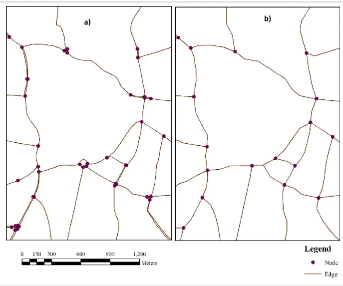
After performing all the preprocessing steps mentioned above, a final clean and simplified road network data was created that was used as the input while implementing the community detection algorithms. The downloaded road network data consisted of 37279 edges and 24124 nodes which was later reduced to 13518 edges and 8214 nodes after data preprocessing steps. Figure 5 shows a small section of the road network before and after the data preprocessing steps.

14

3.4.Implementation of Community Detection Algorithms

Three modularity optimization based algorithms i.e. Louvain, Leiden, and Fastgreedy algorithm were applied in our road network data to identify communities.

3.4.1. Louvain Algorithm

Various python implementation of the Louvain method [28] of community detection can be found as the python modules or packages. We used the python package named 'community' also called 'python-Louvain' [32] which depends on NetworkX [33] for handling graph operations. The input

Figure 5: Small section of the road network data used a) Downloaded road network data b) Road network data after

performing preprocessingsteps

15

graph for this package should be a NetworkX graph object. So, we converted the shapefile of road network data prepared after data preprocessing into NetworkX graph object of nodes and edges by using functions available in NetworkX. We used the both unweighted and weighted graph as input for detecting communities.

For the weighted network, two approaches were used for the partition of nodes. In the first one, the partition of nodes with the highest modularity was identified and this result was used as the major output for most of the analysis. And the second one was used to find partition at different

levels of the dendrogram generated after applying the algorithm.A dendrogram obtained by this

algorithm represents hierarchical clustering of nodes and every level in it is a partition of the nodes. Level 0 is the partition at the lowest level with the smallest communities, and the highest level is 1 less than the length of dendrogram with larger communities and with the maximum modularity.

After the partition of nodes, each community was given a unique identifier which was used to label the communities for later use. These nodes were converted into shapefile format for the post-processing.

3.4.2. Leiden Algorithm

For our research, we used the package named 'leidenalg' [34] as the python implementation of the Leiden algorithm [29]. This package is built on the top of 'igraph' library (https://igraph.org/python/). The input for this algorithm implementation should be a graph of type igraph. We converted the nodes and edges from the networkX graph used in the previous algorithm into an igraph graph to use in this algorithm.

Communities were detected for both weighted and unweighted graphs. It was not possible to obtain the partition of nodes at a different level in this algorithm implementation. So we used the partition obtained with maximum modularity as the output of the algorithm. Since the result obtained using this algorithm were slightly different after each run, the result with maximum modularity among 10 replications was taken for further analysis. The difference in the results for each run is due to the difference in the starting node that this algorithm use for partitioning the nodes. This will lead to the slightly different partitions in different runs of algorithms for which they have optimal modularity. A similar approach used in Louvain algorithm implementation was followed for converting the output into the shapefile of partition nodes with communities' attribute.

16

3.4.3. Fastgreedy Algorithm

We used the python implementation of Fastgreedy Algorithm [30] available in the built-in 'igraph' library named 'community_fastgreedy'. This algorithm finds the communities based on the greedy optimization of modularity. Similar to the Leiden algorithm implementation, we used the weighted and unweighted igraph graph as the input for this algorithm. In this algorithm, we can either specify the desired number of partitions to obtain a fixed number of communities or we can use optimal count option available to obtain communities with maximum modularity. We used the latter option because the number of communities in our case is unknown. The similar approach described in the above two algorithms was used for the conversion of output nodes into shapefile of community partition nodes.

3.4.4. Post-processing of results

The results obtained after implementing community detection algorithms were not directly usable for identifying community areas of city core and hinterlands. So, this step of post-processing was crucial for categorizing the identified communities into core areas and hinterlands. Following steps were involved in the post-processing stage of our research.

3.4.5. Delineation of community areas

The output from the community detection algorithms was the partition of road network nodes. These nodes were saved as shapefiles with the community partition number as attributes. These nodes in the form of points had to be converted into polygon form so that we can identify the core urban and hinterland areas.

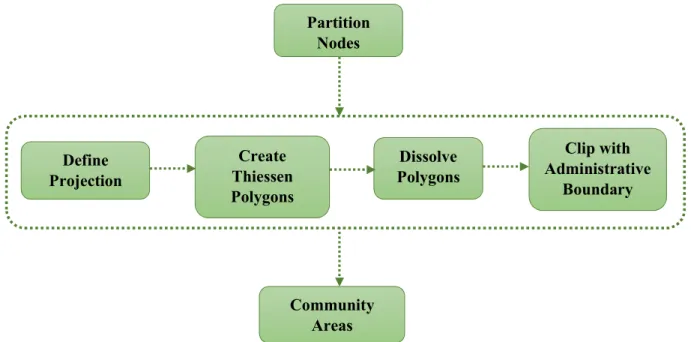
Thiessen polygons were created from the partition nodes obtained as a result of community detection algorithms. These Thiessen polygons were later dissolved based on the community number. All the polygons with the same community number were dissolved and a single polygon was created for each community nodes. As the polygons were formed outside the study area, clipping was done by the administrative boundary to restrict polygons within the study area. The final output of this step was the polygon shapefile containing individual communities. Figure 6 shows the overall process involved in the conversion of partition nodes into community areas.

17

3.4.6. Identifying core urban areas

After converting all the nodes into individual community areas, the next key task was to distinguish between core urban areas and hinterlands. The assumption we considered to identify city cores urban areas was that these areas have a higher density of intersections per kilometer of the road than the rest of the area. The density of intersections in each community was calculated by dividing the total number of nodes inside that community with a total length of road segments (edges) inside the same community.

Road Intersection Density = (3)

After calculating the intersection density for each community, intersection density values were classified into two groups of core areas and others using the Jenks Natural breaks classification. This method is a type of variance-minimization classification. Break values are selected such that it separates the values where large changes in value occur. So it helped to separate the core communities with higher density from the rest of the communities. The range of values obtained for the classification of core areas and others were different across communities areas obtained

Partition Nodes Community Areas Define Projection Create Thiessen Polygons Dissolve Polygons Clip with Administrative Boundary

18

from three implemented algorithms. With the obtained ranges, the detected communities were assigned into core areas and others based on the intersection density value of each community.

We also tried to use a constant range of intersection density to classify the core areas for all the algorithms but this result was not used as the outcome of this research. With this method, all the communities with the value of intersection density greater than 0.61 were assigned as core communities for all the three algorithms.

3.4.7. Assigning city names

After the identification of core urban area communities, the corresponding city name was assigned using reverse geocoding on the core urban communities' centroids. Reverse Geocoding is the process of finding an address for a given latitude and longitude pair. Reverse geocoding was done using the 'Geocoder' python library [35]. OSM Nominatim was used as the provider of geocoding services.

At the end of this step, each core areas were assigned the city name obtained from reverse geocoding. City name of the adjacent core urban communities was assigned to the ones for which city name was not available. Finally, communities belonging to the same city were merged to obtain a single core area polygon of each city.

3.4.8. Identifying Hinterlands

After identifying core urban areas, the remaining communities can be classified as the combination of urban hinterland (or functional region) and other areas. In our research, we focused on detecting the functional hinterland only. We used a simpler approach of adjacency to identify the functional hinterlands among the communities other than core urban areas. In general, the functional hinterlands are in close connection with the core areas of the city. So we identified the communities that are adjacent to core areas as the hinterland of the city. In the case of conflict when a community identified as hinterland is attached to more than one core areas, it was assigned to the core area for which the sum of the weight of connections between that hinterland community and core area is highest. It could be realistic to assign the hinterland community attached to more than one core

19

areas as the common hinterland of connected cities. But, in order to compare the results with OECD Functional Areas, we needed to assign those to only one of the connected core areas.

Hinterland communities that belong to the same city were merged to obtain the single hinterland area for each city.

3.4.9. Comparing Results

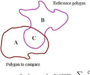
In order to answer two of our research questions, it was essential to compare the results obtained by using different algorithms. To find the similarity of identified core areas and hinterlands among different algorithms and with the OECD functional areas, we used the approach of Goodness-of-Fit (GOF) algorithm developed by Hargrove et. al [36] as the comparison metric. The GOF score proposed in this algorithm can be applied to identify the spatial similarity among entire maps or among vector polygons. The GOF score is unitless and the value ranges from 0 to 1 where 0 signifies no matching at all and 1 signifies completely matching between polygons.

− − ( ) =

+ ∗ +

Sum over all the intersecting polygons

20

In order to compare the results among different algorithms implemented, GOF was calculated for the core areas and hinterland across three algorithms. This helped to recognize the spatial similarity among the core urban areas and hinterlands identified from different algorithms.

For the validation of our results with OECD Functional Urban Areas (FUAs), GOF was calculated between the results obtained using our method with the OECD FUAs. In our study area, OECD data was available for 7 larger cities only. In order to compare the results, the GOF was calculated only for the 7 cities that were available in OECD with the results obtained for these corresponding cities. To find the overall GOF between our results and OECD FUAs, the total core urban area and hinterland of these cities were considered. GOF of individual city core urban areas and hinterland was also calculated to see the similarity between each of the city hinterland pairs identified using our method with OECD FUAs. We excluded the core urban areas and hinterlands of smaller cities that were identified using our approach but were not available in OECD data for comparison.

As there were several results obtained by using different algorithms, abbreviations were used to represent the corresponding results in the next sections of this report.

Table 1: Abbreviations used for different algorithm's results Method

Abbreviations Used

Weighted Network Unweighted Network

Fastgreedy Algorithm FastgreedyWgt FastgreedyNonWgt

Leiden Algorithm LeidenWgt LeidenNonWgt

Louvain Algorithm(Highest Level) LouvainWgt LouvainNonWgt

Louvain Algorithm(Level 3) LouvainWgtLev3 LouvainNonWgtLev3

21

4. Results and Discussion

4.1.Communities detected on the weighted and non-weighted road network

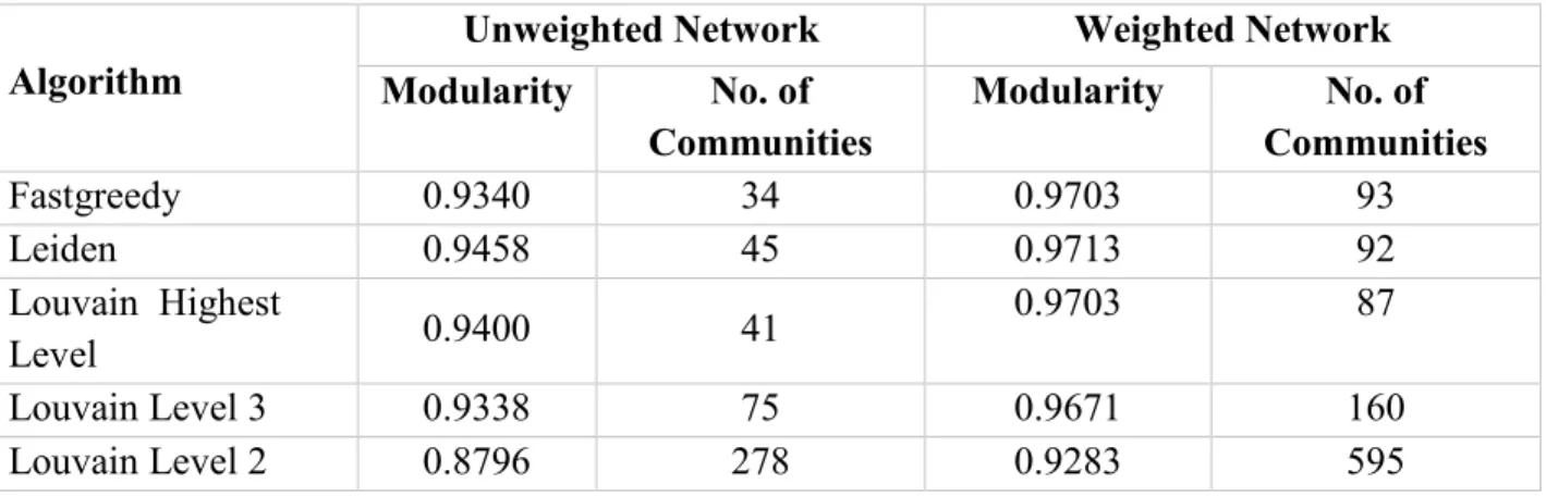
As described in section 3.4, community detection algorithms were implemented on the both unweighted and weighted road network. The modularity scores and the number of communities detected on the road network are shown in Table 2. The number of communities detected on the weighted network is considerably higher than on the unweighted network. Also, the modularity scores are higher in the case of weighted networks for all three algorithms. Leiden algorithm has slightly higher modularity among three algorithms for both weighted and unweighted network. For the Louvain algorithm, communities detected at lower levels show less modularity score and a higher number of communities.

After seeing this result, we can clearly argue that the use of travel time as the weight has a significant effect on the results of community detection algorithms. In general, high modularity indicates a better partitioning of the network into communities. This indicates us that we have a better partition of communities on the weighted network. Also with the increase in a number of communities detected in a weighted network, we can say that the communities detected are with higher resolution (smaller communities are detected).

Table 2: Modularity values and number of communities detected across different algorithms for the unweighted and weighted road network

Algorithm

Unweighted Network Weighted Network

Modularity No. of Communities Modularity No. of Communities Fastgreedy 0.9340 34 0.9703 93 Leiden 0.9458 45 0.9713 92 Louvain Highest Level 0.9400 41 0.9703 87 Louvain Level 3 0.9338 75 0.9671 160 Louvain Level 2 0.8796 278 0.9283 595

22

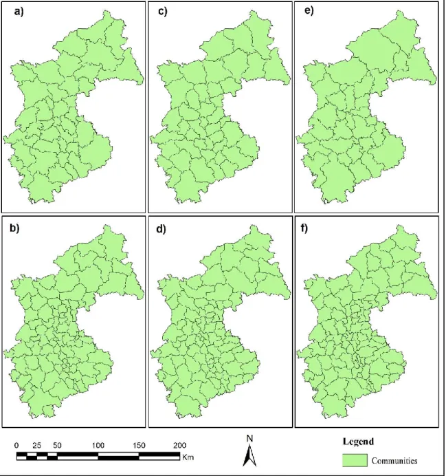
The visual comparison of the communities detected using three algorithms on the weighted and unweighted road network is shown in Figure 8. Size and pattern of communities detected on unweighted road network (Figure 8a, 8c, 8e) are significantly different than that on weighted road networks (Figure 8b, 8d, 8f). In overall, the community areas detected in the unweighted network are larger in size than the community areas detected on a weighted network.

Figure 8: Communities detected on the unweighted and weighted road network by different algorithms. a)LouvainNonWgt b)LouvainWgt c)LeidenNonWeight d)LeidenWgt e)FastgreedyNonWgt f)FastgreedyWgt

23

In the case of unweighted networks, only the number of connections between nodes is considered regardless of longer or shorter road segments connecting them for detecting communities. Thus, it is justifiable to have smaller communities in the weighted network because after using the travel time as a weight factor, the communities are separated mostly by the longer segment of road segments which have more travel time (lesser weight). This helps to identify core areas as separate communities due to the presence of shorter road segments with less travel time (more weight).

The higher density of smaller communities exists in the center and southern part of the study area ((Figure 8b, 8d, 8f). The middle and southern part of the study area constitute of Köln and Düsseldorf region and these regions consist of large cities like Köln, Düsseldorf, Essen, and Duisburg. From this finding, we can at least hint that the presence of smaller and denser communities are significant in the areas where we have a higher density of road networks.

4.2.Classification of city core urban areas and hinterland

The range of intersection density values obtained by using natural breaks for the classification of core urban areas and the number of communities identified as core urban areas in each of the algorithm results is shown in Table 3. The break values obtained for classification of core areas using this approach are not similar across different algorithms. This is justifiable to have this difference in break values because the intersection density values of the communities detected by different algorithms are not similar. Percentage of communities assigned as core urban area in Fastgreedy and Leiden algorithm is a bit higher than that of Louvain algorithm (highest level). Louvain level 2 has the least percentage of communities identified as core areas using this classification.

Methods

Intersection density values for core urban areas (Intersections per Km) No of core communities % of total communities FastgreedyWgt >0.57 33 35% LeidenWgt >0.58 33 36% LouvainWgt >0.62 26 30% LouvainWgtLev3 >0.59 55 34% LouvainWgtLev2 >0.76 131 22%

24

Figure 9 shows the visual comparison of the core urban communities identified using the break values of intersection density obtained as shown in Table 3. Core urban communities are relatively smaller in size and are surrounded by larger communities in the results from three algorithms at the highest level (Figure 9a, 9b, 9c). This signifies that the presence of dense connection of road networks (mostly secondary and tertiary roads) in the city core urban area leads to the detection of smaller communities. As we go farther from the city core, longer segments of primary and

secondary roads are more prevalent leading to the detection of larger communities.Considering

this pattern, we used a simpler concept of adjacency to assign hinterlands by selecting the larger communities around core areas.

Figure 9: Core communities classified using natural breaks classification for different algorithms. a)LouvainWgt ;b)LeidenWgt; c)FastgreedyWgt; d)LouvainLev3Wgt; e)LouvainLev2Wgt

25

In the case of results from Louvain algorithm for lower level, the aforementioned concept of assigning hinterland is not significant as the communities are relatively smaller around the core areas. Also, the modularity score for these methods is lowest among all other which raises the question of reliability of these detected communities. Hence, for detecting hinterlands of the cities, we have only considered the results obtained from FastgreedyWgt, LeidenWgt and LouvainWgt methods.

The hinterlands of each city core urban areas identified are depicted in Figure 10. Altogether 12 core urban areas of the cities and their respective hinterland areas were identified by all the three algorithms. Leiden Algorithm identified one more city core urban area, which was left undetected in other two algorithms Louvain and Fastgreedy.

26

Münster being one of the major city in our study area was left unidentified with our proposed method. This might be due to the issue of resolution limit that these community detection algorithms have. This will be explained in the later section.

4.3.Comparing the results

Table 3 shows the Goodness-of-fit (GOF) scores between the results from three different algorithms and with the OECD FUAs. The average GOF score for core urban areas identified across three algorithms is 0.60 with a standard deviation of 0.10 and for the hinterland areas, the average GOF score is 0.65 with a standard deviation of 0.044. The results from the Leiden algorithm have better similarity with Fastgreedy algorithm with about 70% match for both core urban area and hinterland. These results indicate that the communities detected from different community detection algorithms are quite different which ultimately leads to the identification of dissimilar core urban areas and hinterland of the cities. The results obtained from classification using a constant range of intersection density values is presented in the Appendix.

LouvainWgt LeidenWgt FastgreedyWgt OECD FUAs

LouvainWgt 1 0.64 0.61 0.28

LeidenWgt 0.54 1 0.70 0.37

FastgreedyWgt 0.55 0.72 1 0.28

OECD FUAs 0.43 0.39 0.37 1

GOF Core Area GOF Hinterland

Table 4: GOF values between results from different algorithms and with OECD FUAs

The main reason for the differences in the results is due to the different heuristics used by these algorithms to maximize modularity while identifying communities. As discussed in section 2.4, the Leiden algorithm solves the issues of disconnected communities present in Louvain algorithm and gives a better quality of partition. This improvement in the Leiden algorithm might be one main reason for the difference in communities detected between these two algorithms. Fastgreedy use quite different approach than the other two algorithms. Also, the optimal modularity value achieved as a stopping point for these algorithms during the partition might not be the same. This ultimately leads to the detection of communities that are different across these algorithms. As the community areas detected are different among these algorithms, the intersection density values for

27

these communities will also differ accordingly. Hence, the natural breaks classification identified the non-uniform range of intersection density values for classifying core urban areas across three algorithms. This could be one of the reasons for slightly lower similarity between the core urban areas identified between algorithms.

Comparison of results with OECD FUAs

Overall GOF values obtained after comparing the results from our proposed method with OECD Functional Urban Areas (FUAs) are quite lower for all the three algorithms (Table 4). The average GOF score obtained for core areas is 0.40 with a standard deviation of 0.02 and the average for the hinterland is 0.31 with a standard deviation of 0.04. This result indicates that there is not much similarity between the core areas and hinterland identified using our method with the OECD core areas and hinterland. Among three algorithms, results from Louvain algorithm have highest GOF score of 0.43 for core areas whereas results from Leiden algorithm have the highest GOF score of

0.37 for hinterlands. The overall GOF score was slightly decreased by the influence of the core

urban area and hinterland of Münster city because this city was completely undetected using our method but was included in the OECD FUAs for comparison.

Figure 11 depicts the similarity between the core urban areas obtained from our proposed method and OECD core urban areas of 7 cities. The higher similarity of around 60% is obtained for the core areas of the cities Köln and Düsseldorf by Louvain algorithm. Although similar core urban

Figure 11: Goodness-of-fit scores of core areas identified by three algorithms with OECD core urban areas

0.44 0.33 0.52 0.62 0.41 0.59 0.47 0.32 0.54 0.34 0.46 0.37 0.00 0.52 0.34 0.53 0.56 0.39 0.40 0.00 0.10 0.20 0.30 0.40 0.50 0.60 0.70

Aachen Bonn Duisburg Düsseldorf Essen Köln Münster

GOF Scores of Core areas

28

areas are obtained among the three algorithms for most of the cities, the GOF score appears lower for those cities. In the case of larger cities like Köln and Düsseldorf, the variability between GOF score among the three algorithms seems quite higher. Münster have zero similarity because the core urban area of this city was not detected.

GOF scores between the hinterland identified by our proposed method and the OECD hinterland for 7 cities are depicted in Figure 12. High variability of GOF score can be seen for most of the cities among the hinterlands identified from three algorithms. Essen showed the lowest similarity among all the cities. Münster have the zero similarity for hinterland as well because hinterland can be identified only after identifying core urban area but it was left undetected as mentioned earlier.

Figure 12:Goodness-of-fit scores of hinterland areas identified by three algorithms with OECD hinterlands

In summary, the above results point that city core urban areas and the hinterlands obtained from our proposed method have less similarity with OECD FUAs. It is justifiable to have this difference in the results because OECD uses population data and commuting data of administrative units as the basis to identify core urban areas and hinterlands without considering connectivity through the road network. Hence, we can argue that use of OECD FUAs as the validation data for comparing our result might be unsuitable in our case where the road connectivity is considered as the main

0.34 0.39 0.34 0.57 0.11 0.37 0.40 0.38 _0.37 0.33 0.19 0.59 0.00 0.39 0.59 0.34 0.49 0.09 0.26 0.00 0.10 0.20 0.30 0.40 0.50 0.60 0.70

Aachen Bonn Duisburg Düsseldorf Essen Köln Münster

GOF Scores of hinterlands

29

basis for determining city core urban area and hinterland. OECD method uses employees commuting data of surrounding administrative units to identify hinterland which ignores road network connectivity for people's movement between the city and its hinterland. In our case, we used the assumption that road network topology best represents the connectedness between the city and its hinterland which helped us to determine communities with dense road connections among themselves and sparse connections with the rest. So, using community detection algorithms we were able to detect communities in the road network that can correspond to either core urban area with higher road density and hinterland with lesser road density.

4.4.Resolution limit in Algorithms

In the previous section, we found out that the core urban area of a major city Münster was left undetected due to the resolution limit problem prevailing in modularity optimization algorithms. Due to this problem, algorithms fail to uncover the communities smaller than the certain scale which depends on the total size or weight of the network [27, 37]. In our case, the study area consisted of many larger cities such as Köln and Düsseldorf which have relatively denser road network connections in the core urban areas and were detected easily by these algorithms. But, Münster city although being a major city has relatively few numbers of road network connections within the core urban area and with the surrounding hinterlands as well. As a result, modularity optimization algorithms that we used were unable to detect the core urban area community of Münster as a separate community due to the effect of relatively denser road connection of larger cities existing in the study area.

Figure 13 illustrates this problem of resolution limit where we can see that the algorithms that we use were able to identify smaller communities if the network size is smaller. Figure 13a, 13c, and 13e show the communities detected when the algorithms were applied to the whole study area. Figure 13b, 13d and 13f shows communities detected when the algorithms were applied only on the Münster region with the subset of same road network used for the larger region. Results show that communities detected on the subset of road network have a different result than on the road network of the whole study area. Smaller communities than before are detected in the Münster region after implementing community detection algorithms on the road network of the particular

30

region only. Also, the core urban area of Münster City is detected by all the three algorithms in this scenario (Figure 13b, 13d and 13f) which was left undetected while using the road network of the whole study area. This clearly justifies the earlier statement that the resolution limit problem existing in modularity based community detection algorithms was the main reason for Münster city being undetected in our results.

4.5.Limitations of our work

 In our study, we only used three modularity optimization based community detection algorithms for detecting communities. Use of other algorithms in addition to Modularity based methods could have been used to study the nature of communities detected in road network across different class of algorithms.

Wh ole Stu dy area Mü nster Re gion

31

 As a result of preprocessing steps of the downloaded OSM road network data, underpass and overpass roads were treated as intersections instead of separate links. Although there were very few cases like this, the result could have been improved by retaining such spatial relationship of the road connectivity.

 We only used OECD FUAs as the validation data to compare our results. Due to the lack of more realistic validation data, it was difficult to say which algorithms gave better results in terms of finding city core urban areas and hinterlands. Also, the use of higher modularity values as the basis to choose the results among different methods might not be always true while detecting communities in the real world scenario.

 Due to the rigorous and time-consuming steps for the processing of OSM data, the study area was limited to only three regions of the North Rhine-Westphalia state, Germany. Use of road network of whole state or country for identifying communities could have been considered to get more insights on a different level of city hinterland pair detection.

32

5. Conclusion and future works

With the increasing urbanization, the administrative boundaries used for defining a city no longer portrays the dynamics of urbanization and socio-economic interactions between the city and its surroundings. This has created a challenging task for the geographers to find the right dimension of the city. One way around to this problem could be identifying the city core area and its hinterland as a part of the city itself. Transport network topology being one to represent the connectedness between the city and its hinterland could be utilized as a basis for identifying the city and its hinterland. However, no distinct methodology has been developed to identify hinterlands utilizing road network topology as the main consideration. Hence, this thesis aims to develop and evaluate a methodology for defining city-hinterland pairs at a regional level using community detection algorithms applied to the transport network.

The study of our research was focused on three government regions (Regierungsbezirke) of the North Rhine-Westphalia state, Germany. Firstly, the road network data of the study area was acquired from the freely available OSM dataset. Data preprocessing steps as described in section 3.3 were conducted to obtain a clean and simplified road network data. The road network data prepared after this step was used as an input while implementing community detection algorithms after conversion into a suitable format. Among the various community detection algorithms three modularity optimization based algorithms i.e Louvain algorithm, Leiden algorithm, and Fastgreedy algorithm were used in our research. The results obtained from these algorithm implementations on road network were later processed to recognize communities of core areas and hinterland. The results were compared among the used algorithms and with the OECD Functional Urban Areas.

The results of community detection algorithms implemented on the road network with unweighted and weighted edges were different. Communities detected on unweighted road network had significantly larger communities with coarser resolution and less modularity. In the latter case, smaller communities were detected with higher modularity. This signifies that the use of travel time as weight had a significant effect on our results of community detection algorithms resulting in better partitioning of communities. Results from the algorithms on weighted road network with

33

maximum modularity and at the highest level was utilized to identify core areas and hinterland from the detected communities. Road intersection density of each community was used as a basis for classification of core communities and hinterland. Altogether 12 city core areas were identified by all the three algorithms. The hinterland was identified for each city with the simpler concept of adjacency. Due to the resolution problem existing in these algorithms, one of the main city in our study area was left undetected.

The comparison of results was done with the Goodness-of-fit (GOF) metric developed by Hargrove et. al [36]. Firstly, the result was compared among the implemented algorithms. The average GOF scores for core areas and hinterland areas between results from three algorithms was 0.60 with a standard deviation of 0.10 and 0.65 with a standard deviation of 0.044 respectively. This result was based on the natural breaks classification of core communities. Similarity among the results between the three algorithms was acceptable. The difference in the results could be due to the different heuristics they use to optimize the modularity resulting in a different approximation of maximum modularity value used as stopping criteria of these algorithms.

Secondly, the result obtained from the proposed method was compared with the OECD Functional

Urban Areas.With OECD FUAs the average GOF obtained for core areas was 0.40 with a standard

deviation of 0.02 and the average for the hinterland was 0.31 with a standard deviation of 0.04. The dissimilarity between core areas and hinterland identified with our proposed method with OECD FUAs was obvious as the approach they used for defining core areas was completely different. OECD core areas and hinterland were determined based on population density and commuting data without considering the influence of road connectivity. But, in our case, we considered only the connectedness of the road network as the main basis for identifying city core urban area and hinterland.

In the end, the thesis presented a methodology for detecting cities and their hinterland using community detection algorithms applied on the road network considering the fact that the transport network topology better represents the connectedness between the city and their hinterlands.

34 5.2.Future works

The proposed methodology has much scope for improvement, with more possible scenarios to be explored. Following possible ways of improvement are recommended for future research.

 Modularity-based community detection algorithms used in our research use Newman-Girvan null model for maximizing modularity. This null model doesn’t take into account any problem-specific constraints (such as distance) to randomize the network in the case of spatial networks [37]. So, future research could involve modification of this null model by incorporating such information while detecting communities in the road network.  Further studies can be carried out in terms of validating the results obtained from our

approach with more realistic validation data of city-hinterland pairs.

 In this thesis, we considered using only road network data. Use of railway network in addition to road network is recommended for improved results.

 Use of different level of roads network data could be useful in the case when we want to identify a hierarchy of cities and hinterlands by identifying communities at different scale.  We considered detecting only functional hinterland. Future research could focus on

identifying rural hinterland of the cities which are beyond the functional regions.

35

Bibliography

[1] United Nations, “World Urbanization Prospects: The 2018 Revision,” World Urban.

Prospect. 2018 Revis., pp. 1–2, 2018.

[2] D. Sanchez-Serra, “Functional Urban Areas in Colombia,” 2016.

[3] H. Sukopp, “Urban ecology—scientific and practical aspects,” in Urban ecology, Springer,

1998, pp. 3–16.

[4] A. Fenton, “Urban Area and Hinterland : Defining Large Cities in England , Scotland and

Wales in terms of their constituent neighbourhoods,” no. April 2013, 2015.

[5] F. Krausmann and L. S. Vienna, “A City and Its Hinterland : Vienna ’ s Energy Metabolism

1800 – 2006 A City and its Hinterland : Vienna ’ s Energy Metabolism 1800-2006,” no. September 2013, 2014.

[6] B. J. Dermody, M. Sivapalan, E. Stehfest, D. P. Van Vuuren, and M. J. Wassen, “A

framework for modelling the complexities of food and water security under globalisation,” pp. 103–118, 2018.

[7] A. Allen, A. Allen, P. Mcalpine, M. Chabra, and A. Minaya, “Environmental planning and

management of the peri-urban interface : perspectives on an emerging field,” vol. 15, no. 1, pp. 135–148, 2003.

[8] K. Hoggart, “City hinterlands in European space,” in The City’s Hinterland, Routledge,

2016, pp. 11–28.

[9] B. Schuh and S. Sedlacek, “City, Hinterlands-Sustainable Relations,” 2000.

[10] M. Brezzi, M. Piacentini, K. Rosina, and D. Sanchez-Serra, “Redefining urban areas in OECD countries,” Redefining" urban" a new W. to Meas. Metrop. areas, OECD, Paris, FR, pp. 19–58, 2012.

[11] M. Barthélemy, “Spatial networks,” Phys. Rep., vol. 499, no. 1–3, pp. 1–101, 2011.

[12] M. E. J. Newman and M. Girvan, “Finding and evaluating community structure in networks,” Phys. Rev. E, vol. 69, no. 2, p. 026113, Feb. 2004.