The Economic Effects of Public Financing:
Evidence from Municipal Bond Ratings Recalibration
*Manuel Adelino
Duke University
Igor Cunha
University of Kentucky
Miguel A. Ferreira
Nova School of Business and Economics, ECGI
Abstract
We show that municipalities’ financial constraints can have a significant impact on local employment and growth. We identify these effects by exploiting exogenous upgrades in U.S. municipal bond ratings caused by Moody’s recalibration of its ratings scale in 2010. We find that local governments increase expenditures because their debt capacity expands following a rating upgrade. These expenditures have an estimated local income multiplier of 1.9 and a cost per job of $20,000 per year. Our findings suggest that debt-financed increases in government spending can improve economic conditions during recessions. (JEL E24, G24, G28, H74)
* We thank Andrew Karolyi (the editor), two anonymous referees, Heitor Almeida, Jean-Noel Barrot, Daniel
Bergstresser, Bernard Black, Dario Cestau, Gabriel Chodorow-Reich, Jess Cornaggia, Kimberly Cornaggia, Michael Faulkender, Fernando Ferreira, Tracy Gordon, Todd Gormley, John Griffin, Ryan Israelsen, William Mullins, Hoai-Luu Nguyen, Felipe Restrepo, and Ruy Ribeiro; participants at the American Finance Association Annual Meeting, Carnegie Mellon Conference on the Economics of Credit Rating Agencies, CEPR European Summer Symposium in Corporate Finance, European Finance Association Annual Meeting, SFS Cavalcade, Brandeis Municipal Finance Conference, and Lubrafin; and seminar participants at Cornell University, Federal Reserve Bank of Chicago, FGV– São Paulo School of Economics, Harvard Business School, Indiana University, Insper, London Business School, Maastricht University, Norwegian School of Economics, Nova School of Business and Economics, Texas A&M, Tilburg University, and University of Amsterdam for helpful comments. Financial support from the European Research Council (ERC) and the Fundação para a Ciência e Tecnologia (FCT) is gratefully acknowledged. Send correspondence to Miguel Ferreira Nova School of Business and Economics, Campus de Campolide, 1099-032 Lisboa, Portugal; telephone: +351 213801631; e-mail: [email protected].
1
Municipal bond markets are an important source for state and local governments to finance the construction and maintenance of infrastructure and other public projects, provide cash flow for government needs and services, and finance private projects (using conduit financing). According to the U.S. Securities and Exchange Commission (SEC 2012), as of December 2011, investors held more than one million municipal bond issues, representing an outstanding (principal) amount of more than $3.7 trillion, or about 25% of the gross domestic product (GDP) of the United States.
In this paper, we examine how changes to the supply of credit to municipalities in the United States affect local economies, particularly during recessions. Easier access to financing can have important effects on economic outcomes when governments face financial distress, such as during the 2007–2009 Great Recession.1 Specifically, local governments can use bond financing to alleviate spending cuts, prevent tax and fee increases, or contribute to their end-of-year balances. These increases in government spending can either have positive spillover effects in the private sector arising from increased disposable income or crowd out private consumption and investment.
We identify the real effects of public financing by exploiting exogenous variation in U.S. municipal bond ratings due to Moody’s 2010 recalibration of its municipal bond rating scale. Before the recalibration, Moody’s had a dual-class rating system. Moody’s Municipal Rating Scale measured distance to distress (i.e., how likely a municipality is to reach a weakened financial position that requires extraordinary support from a higher level of government to avoid default). Moody’s Global Rating Scale, in contrast, measures expected losses (i.e., default probability and loss given default) among sovereign and corporate bonds. This dual-class rating system persisted for decades until Moody’s recalibrated its Municipal Rating Scale to align it with the Global Rating Scale in April–May 2010. As a result, nearly 18,000 local governments received ratings upgrades of up to three notches, corresponding to bonds worth more than $2.2
1 According to the 2009 Surveys of State and Local Finances conducted by the Census Bureau, during the 2009
2
trillion in par value (nearly 70,000 bond issues).
Moody’s recalibration allows us to isolate changes in economic outcomes that are caused by changes in public financing from those that would occur absent of these changes. The upgrades that resulted from the recalibration did not reflect changes to the issuers’ intrinsic quality, but rather the goal of aligning municipal ratings standards with those of sovereign and corporate ratings. In fact, the recalibration algorithm used expected losses by rating level and type of government, and thus changes in ratings due to the recalibration are uncorrelated with changes to local government (and nationwide) fundamentals. An important aspect of the recalibration is that it did not affect all local governments. Local governments that were already properly calibrated vis-à-vis the Global Rating Scale can be used as a control group. In addition, local governments without Moody’s rating or with the maximum attainable rating (i.e., Aaa rating) were, by definition, not subject to recalibration and can also be used as a control group. To ensure comparability of treatment and control groups, we restrict the sample to local governments that issued bonds during the four-year period before the recalibration.
We employ a difference-in-differences approach to compare the outcomes between upgraded local government units (the treatment group) and non-upgraded local government units (the control group) around the recalibration. We study how this shock to municipal ratings affects outcomes at both local government and county levels. Because our event affects bonds issued by any local government unit within a county (i.e., the recalibration can affect bonds issued by counties, cities, townships, school districts, and special districts), we aggregate all changes in ratings in a county whenever we study county-level outcomes.2 Our treatment (continuous) variable is the fraction of local government units in each county whose outstanding bonds were upgraded because of the recalibration. The specifications include county-level control variables, as well as by-year fixed effects to capture any source of time-varying unobserved state-level heterogeneity, such as changes in transfers from state governments and ballooning of unfunded state pension liabilities. We also estimate specifications with county-size decile-by-
3
year fixed effects to account for the possibility that the Great Recession and the subsequent recovery may have affected large and small counties differently.
We first examine whether Moody’s recalibration causes an asymmetric effect in the ratings of new municipal bond issues in the primary market during the 2006–2013 period. We find that Moody’s ratings increase 0.7 notches more for upgraded local governments than for non-upgraded local governments. We use S&P municipal bond ratings as a placebo test for the sample of bonds that have both Moody’s and S&P ratings (about 55% of the bonds). If the recalibration by Moody’s reflects changes in underlying credit quality, the S&P ratings on this sample of bonds would also be affected. We find no significant changes in the S&P ratings between the treatment and control groups.
We also find that upgraded local governments increase the amount of new bond issues significantly relative to non-upgraded local governments following the recalibration. The differential effect on the amount of bonds issued (at the local government level) is 16%–20% per year in the three-year period after the recalibration (April 2010–March 2013) relative to the four-year period before the event (April 2006–March 2010). At the county level, a one standard deviation increase in the fraction of upgraded local governments increases the amount of bonds issued by 3.1%. The offer yield of the new bond issues of upgraded local governments decreases by 14 basis points relative to non-upgraded local governments. These findings are consistent with credit ratings playing an informational role in the municipal bond market. This may be due to the larger presence of retail investors relative to other fixed-income markets, which means that ratings are more likely to be used as a source of information.3 The effects may also be the result of ratings-based regulations and internal policies on institutional investors.4 Our offer yield
3 According to the U.S. Flow of Funds Accounts quarterly data, the household sector held $1,872 billion of the
$3,772 billion of municipal bonds outstanding in 2010 (a share of almost 50%). This share decreased to about 44% by 2013, but households still have an important share of the municipal bond market. In contrast, households held only 19% of corporate and foreign bonds as of 2010.
4 Beyond official regulations (e.g., Basel II and National Association of Insurance Commissioners (NAIC)
guidelines), investment management policies and practices often rely on ratings by restricting the portfolio holdings of institutional investors (e.g., Chen et al. 2014). In the aftermath of the 2007–2009 financial crisis, several
4
results are consistent with those in Cornaggia, Cornaggia, and Israelsen (2015), who use the Moody’s ratings recalibration to study the effects of credit ratings on municipal bond prices. They find that upgraded bonds earn abnormal returns in the secondary market, and that upgraded municipalities subsequently benefit from a reduction in offer yields in the primary market. Our study builds on the results in Cornaggia, Cornaggia, and Israelsen (2015) to study how a shock to local governments’ financial constraints, caused by the ratings recalibration, affects the real economy in terms of government spending, employment, and income.
Consistent with local governments using the additional bond financing to improve economic conditions, we find significant effects on local economic outcomes after the recalibration. We find that a one standard deviation increase in the fraction of local governments upgraded in a county increases local governments’ expenditures and employment by 0.5%. Even though state and local governments are required to have balanced budgets, court decisions and referendums on borrowing have led to the exclusion of (capital) expenditures funded by long-term debt from deficit calculations as reported by the National Conference of State Legislatures (2003). There is also de facto flexibility for local governments to run deficits (at least for limited periods).
We find evidence of spillover effects to private employment and income measured at the county level. A one standard deviation increase in the fraction of local governments upgraded in a county increases total private employment by 0.3%. We also find that the effects on private employment are heterogeneous across sectors and are concentrated in the non-tradable sector (retail, food, and accommodation), which depends primarily on local demand, and in the education sector, which typically receive transfers or grants from local governments. A one standard deviation increase in the fraction of local governments upgraded in a county increases non-tradable employment by 0.9% and education sector employment by 1%. The effect in the tradable sector is statistically insignificant. Last, we find that county-level income increases in response to the recalibration event. A one standard deviation increase in the fraction of upgraded
regulatory initiatives have been taken to reduce the mechanical reliance on credit ratings by market participants (the 2010 Dodd-Frank Wall Street Reform and Consumer Protection Act; and Financial Stability Board 2010, 2012).
5
local governments increases income by 0.5%.
The effect of the recalibration is heterogeneous across municipalities. The results are more pronounced in the sample of high leverage, low rating, and small local governments units, consistent with the recalibration playing a particularly important role for financially constrained local governments. We also find that results are stronger in counties with higher unemployment rate, consistent with the idea that expansionary government spending is less likely to crowd out private consumption or investment in an economy with greater economic slack.
Our results are robust to a series of alternative sample definitions and specifications to guarantee that the results are not driven by a lack of comparability between treatment and control groups. We obtain consistent estimates when we restrict the sample to counties located in urban areas, counties with multiple bond issuers, and counties with higher amount of bonds issued. We also obtain consistent estimates when we include group-specific (treatment and control) trends, which mitigates concerns about pre-existing differential trends.
Our study contributes to the literature that relies on cross-sectional variation in the estimation of local fiscal multipliers (e.g., Cohen, Coval, and Malloy 2011; Chodorow-Reich et al. 2012; Nakamura and Steinsson 2014; and Suarez-Serrato and Wingender 2014), which differs from the traditional empirical macroeconomics literature, where time series variation is employed (see Ramey 2011 for a survey). The long-standing debate on the effects of public spending on economic outcomes and the size of the fiscal multiplier has received additional attention due to the American Recovery and Reinvestment Act (ARRA) of 2009.
Given that we exploit a cross-sectional regional shock to government financing and expenditures, we can provide estimates of local fiscal multipliers (the “open economy relative multiplier”)—that is, the effect that a relative increase in government spending in one region relative to another has on relative output or employment. A caveat of this approach is that it ignores general equilibrium effects, which could change the interpretation of the overall effect of the stimulus spending and national multiplier (the “closed economy aggregate multiplier”).
6
estimate that a marginal million dollars in local government expenditures results in an additional 51 jobs, 45 of which are outside the public sector. This estimate corresponds to a cost per job created of $20,000 per year. Our estimates also imply an income multiplier of 1.9 (i.e., dollar change in local income produced by a one-dollar change in local government spending). Combining the income and employment multipliers, we estimate that the jobs created have a remuneration of 1.9 × $20,000 = $38,000 per year.
Our estimates of fiscal multipliers are in line with the estimates of local fiscal multipliers in the literature. This is consistent with Keynesian models that predict high multipliers during periods when the marginal propensity to consume is high. Intuitively, in periods of factor underutilization and when interest rates are near zero, government spending shocks are less likely to crowd out private consumption and investment, and fiscal multipliers should thus be larger (e.g., Auerbach and Gorodnichenko 2012; and Fishback and Kachanovskaya 2015).5
We also contribute to the literature on the effect of credit market shocks on economic outcomes. Mian and Sufi (2011, 2014) and Mian, Sufi, and Rao (2013) focus on the role of household leverage in explaining the severity of the Great Recession in 2007–2009, and Giroud and Mueller (Forthcoming) focus on the role of firm leverage. Chodorow-Reich (2014) shows that firms with pre-crisis lending relationships with weaker banks face restrictions in credit supply and reductions in employment following the collapse of Lehman Brothers in 2008. Greenstone, Mas, and Nguyen (2014) and Bentolila et al. (Forthcoming) find that shocks to the supply of bank credit to (small) businesses during the Great Recession are associated with reductions in employment.6 Whereas these authors study the economic effects of credit supply shocks to the private sector, we study the economic effects of credit supply shocks to the public sector. To the best of our knowledge, we are the first to provide causal evidence of the real effects of municipal bond markets.
5 The ratings recalibration coincided with a period with significant slack in the economy and short-term interest rates
near zero. In December 2009, the real GDP annual growth was -2.8%, the unemployment rate was about 9.9% (both drawn from the Bureau of Economic Analysis), and the federal funds rate was 0.12%.
6 Others study the effect of credit expansions (through mortgage origination) on house prices and (non-tradable)
7
Last, we contribute to the literature on the real effects of credit ratings. Credit ratings matter for firm investment and financial policy (Faulkender and Petersen 2006; Kisgen 2006, 2009; Sufi 2009; Tang 2009; Kisgen and Strahan 2010; Chernenko and Sunderam 2012; Manso 2013; and Almeida et al. 2017).
1. Institutional Background and Data
1.1 Recalibration Event
Moody’s had a dual-class rating system before the ratings recalibration in 2010. Moody’s Municipal Rating Scale measured distance to distress (i.e., how likely a municipality was to reach a position that required support from a higher level of government to avoid default). In contrast, Moody’s Global Rating Scale is designed to measure expected losses (default probability and loss given default) among sovereign bonds, corporate bonds, and structured finance products (Moody’s 2007). Moody’s (2009) attributes its dual-class rating system to the preferences of the highly risk-averse investors in municipal bonds.According to the Flow of Funds Accounts in 2010, households owned 50% of municipal bonds, followed by money market funds with 10% and insurance companies with 9%. In contrast, households held only 19% of corporate and foreign bonds.
Moody’s dual-class rating system produced lower ratings for municipal bonds relative to its competitors. In our sample, Moody’s assigned a rating lower than S&P in 53% of the issues (and the same rating in 40% of the issues) in the year before the recalibration; this number drops to only 17% in the year after the recalibration (reflecting the upgrades). In addition, Moody’s (2007) shows that default rates in municipal bonds are significantly lower than those experienced by comparable corporate bonds. Because of the more conservative ratings under the dual-class system, Moody’s share in the municipal bond market declined. In the year before the recalibration, Moody’s had a market share of 34%, compared with S&P’s share of 59% and Fitch’s share of 7%. After the recalibration, Moody’s market share increased to more than 40%
8
(2010–2012).7
Moody’s maintained a sizable market share despite this apparent competitive disadvantage under the dual-class system likely because many regulations (e.g., Basel II and National Association of Insurance Commissioners (NAIC) guidelines) and investment rules require at least two ratings from a nationally recognized statistical rating organization (NRSRO), and use the lower of two ratings, or the middle of three ratings, as the basis for regulatory benchmarks (e.g., banks’ capital requirement).8 Beyond regulations, local governments’ debt management policies and institutional investors’ policies often require two ratings. For example, the County of Alameda (2014), California, debt management policy stipulates that “at least two credit ratings should be procured from any of the nationally recognized credit rating services, unless the transaction is of a small size.”9 The Government Finance Officers Association (2015) (GFOA) also writes that “historically, many issuers have sought separate ratings from at least two credit rating agencies. In addition, many institutional investors require a minimum of two ratings.” Market participants also emphasize the importance of two ratings. Timothy Cox, executive director of debt capital markets at Mizuho Securities, said in an interview with Bloomberg (2011): “If I don’t have two ratings on a bond, I cannot sell it. No money manager is going to buy it.”
Moody’s intention to map municipal bond ratings into the Global Rating Scale dates back to at least 2002 (Moody’s 2002) and is mentioned in a variety of publications over the years. Moody’s issued a request for comments from market participants about the methodology and a potential shift from the municipal scale to the global scale in June 2006 (Moody’s 2006). It planned to implement the ratings recalibration in June and July 2008, but the financial market
7 Moody’s also faced lawsuits over its dual-class rating system arguing that harsher standards imposed on
municipalities resulted in higher borrowing costs for taxpayers.
8 Bongaerts, Cremers, and Goetzmann (2012) find that Fitch typically plays the role of a “third opinion” (in addition
to Moody’s and S&P ratings), which matters primarily for regulatory purposes, rather than providing additional information about credit quality. Becker and Milbourn (2011) find that increased competition from Fitch is associated with higher and less informative ratings from the incumbents (Moody’s and S&P).
9 As another example, in 2008 the attorney general of the state of Connecticut stated in a letter to Barney Frank
(chairman, House Committee on Financial Services): “The credit rating market is highly concentrated and most issuers require two ratings from a NRSRO to make their bond marketable under SEC rules.”
9
turmoil during the summer and fall of 2008 led to a postponement. Finally, in March 2010, Moody’s announced a recalibration of its Municipal Rating Scale to align it with the Global Rating Scale (Moody’s 2010). In April and May 2010, over a four-week period, Moody’s announced how individual bonds would be affected by the recalibration, resulting in a zero-to-three-notch upgrade of nearly 70,000 bond ratings.
Moody’s recalibration algorithm used the expected losses by rating level and type of government (i.e., historical default rates by rating level and loss severity by government type) to map to its equivalent rating on the global scale. An important aspect of this recalibration is that not all municipal bond issues were upgraded and therefore can be used as control group. Some local governments were already properly calibrated vis-à-vis the global scale, in particular special districts related to housing and health-care did not see a change in ratings. In addition, bonds with higher ratings (at or above Aa3) on the municipal scale were less likely to be recalibrated than those with a lower rating (below Aa3); bonds with the maximum attainable rating (Aaa) in the municipal scale could, by definition, not be upgraded. Of course, local governments without bonds rated by Moody’s were not subject to recalibration and can also be used as a control group.
Moody’s (2010) clarifies that the recalibration is intended to enhance the comparability of ratings across asset classes, and it does not indicate a change in the credit quality of the issuer: “Our benchmarking … will result in an upward shift for most state and local government long-term municipal ratings by up to three notches. The degree of movement will be less for some sectors … which are largely already aligned with ratings on the global scale. Market participants should not view the recalibration of municipal ratings as ratings upgrades, but rather as a recalibration of the ratings to a different scale … (The recalibration) does not reflect an improvement in credit quality or a change in our opinion.”
Moody’s (2010) also reports that any ratings under review for upgrade or downgrade before recalibration would remain under review and would not be lumped into these rating changes. Thus, our sample does not include any natural upgrades associated with improving issuer
10
fundamentals that could contaminate our results. In addition, because the methodology closely follows a discussion that occurred (and was made public) over a period of several years, it is especially unlikely that the rating changes could include information about individual local governments.
1.2 Data
We obtain a list of recalibrated bond issues from Moody’s. The list contains the rating of each bond issue before and after the recalibration, with the change in rating ranging from zero to three notches. The recalibration comprised 69,657 municipal bonds (with a total par amount of $2.2 trillion). Almost all the bonds had an investment-grade rating before the recalibration (only 56 municipal bonds had a speculative-grade rating).
The municipal bond market data come from the Ipreo i-Deal new issues database. The sample period is from April 2006 to March 2013, which corresponds to the four-year period before the recalibration and the three-year period afterward. We restrict the sample to local governments that issued bonds during the four-year period before the recalibration.10 We exclude from the sample bond issues from special districts in the housing and health-care sectors because they were already properly calibrated relative to the global rating scale and did not see a change in ratings.11 Bonds issued by upgraded local governments (i.e., an issuer that experienced an upgrade in any of its outstanding bonds due to Moody’s recalibration) represent about 74% of the sample of new issues (53% were upgraded by up to one notch, 19% by two notches, and 2% by three notches).
Because we measure economic outcomes (private employment and income) at the county level, we restrict the analysis of the recalibration to bond issues that can be matched to a county. These include issues by counties (including boroughs and parishes), cities, townships (including
10 We obtain numerically identical differential effects when we include all new issues or restrict the sample of new
issues to local governments that issue bonds both before and after the recalibration, given that only local governments that issue bonds both before and after can be identified with the difference-in-differences estimator.
11 These sectors represent about 21% of the bond issues from special districts. We obtain similar estimates when we
11
towns and villages), school districts, and special districts. We exclude state-level bonds because they cannot be linked to a specific county. Because credit ratings on insured bonds reflect the credit quality of the insurer rather than the issuer, we include only uninsured bonds in our analysis (roughly 60% of bonds).
The primary economic outcome variables are local government expenditures, government employment, private employment (total and for sectors), and income. We obtain data on government expenditures from the U.S. Census Bureau’s Annual Survey of State and Local Government Finances. The data include revenues and expenditures of individual local government units within each county. The sample includes local governments that are present in all years of our sample period (2007–2013).
We obtain local government employment data from the Census Bureau’s Government Employment and Payroll Survey. The Census Bureau conducts a complete census of local government employees every five years (e.g., 2002, 2007, 2012), and a sample of local governments is used in the other years. Government employment is measured as full-time-equivalent employees at local government units within each county as of the week of March 12 of each year. The analysis of local government employment is restricted to local government units that are present in all years of our sample period (2007–2013).12
We obtain data on private-sector employment by industry (National American Industry Classification System (NAICS)) and county from the County Business Patterns (CBP) published by the Census Bureau. The data include employment in the week of March 12 of each year. We also present results using data on quarterly employment from the Census Bureau’s Quarterly Workforce Indicators (QWI). The QWI is derived from the Longitudinal Employer-Household Dynamics (LEHD) program at the Census Bureau. We obtain county-level income data from the Internal Revenue Service (IRS) Statistics of Income. Income is defined as total wages and salaries in a given county and calendar year (the sample period for income is 2006–2012).
12 The sample of counties with government employment data includes only 1,618 counties, which corresponds to
12
In our tests, we control for other factors that are important determinants of local economic conditions. We include yearly changes in house prices (to capture the severity of the post-2006 downturn in each county), as well as the number of households. The housing prices come from the Federal Housing Finance Agency’s (FHFA’s) House Price Index (HPI) data at the Metropolitan Statistical Area (MSA) level. The HPI is a weighted repeat-sales index that measures the average price changes in repeat sales or refinancing on the same properties.13 We obtain county-level information on the number of households, defined as one or more people who occupy a given housing unit, from the 2007 Census Bureau Summary Files.
1.3 Summary Statistics
Panel A of Table 1 presents summary statistics on county-level outcome variables from 2007 to 2013. Our sample consists of counties in which at least one local government issued bonds in the municipal bond market in the four-year period before the recalibration (April 2006–March 2010). Thus, the local governments in the control group either do not have a rating from Moody’s (i.e., they were rated only by S&P or Fitch) or have a Moody’s rating that was not affected in the recalibration. This sample of bond issuers comprises 1,768 counties for which we also have employment and income data, which correspond to about 60% of the counties in the United States.14
We map the ratings into 22 numerical values, where 22 is the highest rating (Aaa), 21 the second highest (Aa1), and one the lowest (default). The average numerical rating by Moody’s is 17.9, corresponding to a rating between A1 and A2. The median is 18 (A1). About half of our sample of new issues rated by Moody’s is simultaneously rated by S&P. The average numerical rating by S&P is 18.6, confirming that Moody’s municipal bond ratings were lower than S&P ratings before the recalibration. Counties in the sample issue an average of $170 million in bonds
13 Whenever the MSA HPI is missing, we complement the data with state-level house price indices from the FHFA. 14 The number of counties included in each regression varies according to the availability of sector-level
employment-by-county data in the CBP. The Census Bureau often omits observations, or includes only broad ranges, for confidentiality reasons.
13
each year, but the distribution is highly skewed with a median of $15 million. The offer yield is 2.8% on average.
Counties in the sample have an average of 6,200 government employees and a median of 1,370 government employees. The average county in the sample has local government expenditures of $766 million. The distribution is also heavily skewed, with a median of $143 million dollars.
Private employment in each county is much larger than government employment at 60,170 employees on average. We separately track tradable and non-tradable employment based on two-digit NAICS codes. Average employment in the tradable sector (manufacturing; NAICS codes 31–33) is 4,390 employees, while average employment in the non-tradable sector (retail, food and accommodation; NAICS codes 44–45 and 72) is about 14,020 employees.
The final row of Table 1 presents summary statistics on the main explanatory variable (Recalibrated) at the county level. We first define the treatment and control groups at the local government level. The treatment group contains local governments whose outstanding bonds were upgraded during the Moody’s recalibration event. We then calculate our treatment (continuous) variable at the county level as the fraction of all local government units in a given county that were upgraded due to the Moody’s recalibration (Recalibrated). Figure 1 shows a map of the United States with the terciles of the Recalibrated variable (among those counties with non-zero value), which are well spread across the United States.
Panel B of Table 1 presents summary statistics on county-level outcome variables for an alternative sample. Specifically, we focus on the sample of urban counties (those counties with more than 50,000 people following the Census Bureau definition). This sample of urban counties comprises 933 counties, and the counties are, on average, bigger than those in Panel A. For example, counties in the sample of urban counties have an average of 93,620 households versus an average of 53,280 in the sample of bond issuers.
Table 2 provides a comparison of counties with recalibrated local governments (i.e., counties with non-zero Recalibrated variable–the treated counties) and counties without recalibrated local
14
governments (i.e., counties with Recalibrated variable equal to zero−the control counties) in the pre-recalibration period. Because the median of Recalibrated is zero, recalibrated counties correspond to the counties with above-median Recalibrated, whereas non-recalibrated counties correspond to the counties with below (or at)-median Recalibrated. The sample in Panel A consists of counties with bond issuers, and the sample in Panel B consists of urban counties.
Panel A shows that one feature of the data is that counties in the treatment group are larger than counties in the control group. The average number of households is 82,120 for the treatment group versus 19,410 for the control group. The average total private employment presents a similar pattern with 97,520 and 18,620 for treatment and control groups, respectively. We present both raw differences in means between treatment and control groups, as well as differences after adjusting for state-by-year and county-size decile-by-year fixed effects. This adjustment controls for regional and size heterogeneity in a given year between treatment and control groups, and the differences in number of households and private employment are no longer statistically (or economically) significant. We use this strategy in the regression tests to ensure comparability of treatment and control groups along the regional and size dimensions (as well as to absorb any time-varying factors that could affect counties of distinct sizes differently). Panel A also shows that the treatment and control groups have similar economic structures in terms of relative importance of local government employment versus private employment. Additionally, the growth rates (annual log change) of outcome variables in the pre-treatment period are similar across the two groups, except for government expenditures. These differences become relatively smaller in Panel B, when we make the comparisons within urban counties.
2. Effect on Municipal Bond Market
We start by examining the effects of the ratings recalibration on the access of local governments to the municipal bond market. We study the effect of Moody’s recalibration on bond ratings, as well as on quantities and prices in the municipal bond market. We estimate the equivalent of a first stage in our setting (given that we are primarily interested in economic
15
outcomes) by comparing the ratings, amount of bonds issued, and offer yield of upgraded local governments (the treatment group) and non-upgraded local governments (the control group) in the three-year period after the recalibration relative to the four-year period before.
We first estimate the effects of the recalibration on ratings aggregated to the county level. We aggregate the new bond issues data using the average rating across all issues in each county and event year. We estimate the following (reduced form) regression:
, , , (1)
The analysis is conducted within-county—that is, we include county fixed effects ( ) in all regressions. The regressions include state-by-year fixed effects ( , , as well as county-size decile-by-year fixed effects in some specifications ( , ). The explanatory variable of interest is the fraction of upgraded local governments in a county (Recalibrated) interacted with a dummy variable that takes a value of one for April 2010–March 2013 (Post). The fixed effects (county and state-by-year fixed effects) absorb both the Recalibrated and the Post dummy variables. We also control for issue characteristics, including whether the bond is a general obligation (GO) bond or revenue bond, whether the bond is part of the Build America Bonds (BAB) program, and duration.15 Standard errors are clustered at the county level to correct for within-county residual correlation.
Panel A of Table 3 presents the results of county-level regressions of the effects on ratings. Column (1) presents the results in which the dependent variable is the Moody’s rating. We find that the coefficient of the interaction term Recalibrated Post is positive and significant. Column (2) shows a similar differential effect on ratings when we include county-size decile-by-year fixed effects in the regression. When we use the sample of urban counties in columns (5) and (6), the effects are slightly weaker but statistically significant.
15 The BAB program ran from April 2009 to December 2010 to help state and local governments regain access to
the bond markets and invest in infrastructure projects after the financial crisis. Our sample contains 4% of the bonds that are part of the BAB program. General obligation bonds represent 50% of the sample of bonds, and revenue bonds represent the other 50%.
16
About half of our sample of new issues rated by Moody’s is simultaneously rated by S&P. We can use the S&P ratings as a placebo test, because S&P does not have a dual-class rating system. Specifically, this allows us to test whether the effect on Moody’s ratings is the result of information about the creditworthiness of the upgraded municipalities (in which case S&P ratings should also react). Columns (3) and (4) of Table 3 show no significant differential effect on S&P ratings between the treatment and control groups following the recalibration. When we use the sample of urban counties in columns (7) and (8), the effects on S&P ratings are also statistically insignificant. Although the exclusion restriction is not directly testable, we view this finding as an important validation of our identification strategy.16
Panel B of Table 3 presents the results of local government–level regressions of the effects on ratings. The dependent variable is the average rating across all issues of a given local government in each event year. We estimate the following (reduced form) regression:
, , , (2)
The main explanatory variable of interest is the interaction term Recalibrated Dummy Post. The Recalibrated Dummy takes a value of one if local government j experienced an upgrade in any of its outstanding bonds during the Moody’s recalibration event. The analysis is conducted within local governments (issuer)—that is, we include local government fixed effects ( in the regressions. The regressions also include government type-year fixed effects ( , and county-year fixed effects ( , . Standard errors are clustered at the local government level to correct for within-local-government residual correlation.
The local-government-level results in Panel B are similar to the county-level results in Panel A. We find that the coefficient of the interaction term Recalibrated Dummy Post is positive and significant, which indicates that the recalibration has a disproportional effect of about 0.7 notches on the Moody’s ratings of the treatment group relative to the control group. In addition,
16 We find that the interaction term Recalibrated Post coefficient remains positive and significant in the sample of
17
there is no evidence of a significant differential effect on S&P ratings.
Figure 2 shows the effect of the recalibration on Moody’s ratings for the treatment and control groups from three years before the recalibration to three years after it (relative to four years before the recalibration, the baseline year). Treatment and control groups show no significant differential changes before the recalibration. The treatment group undergoes a significantly larger increase in ratings at the time of the recalibration, a difference that persists for up to three years. Figure 3 also shows that there are no significant changes in the S&P ratings of the treatment and control groups either before or after the recalibration, confirming that channels other than ratings do not seem to drive our effects.
We also estimate the effect of the recalibration on ratings at the bond issue level. Table IA.1 in the Internet Appendix presents the results, which are similar to the county-level and local-government-level results in Table 3. Table IA.2 shows that the results are robust when we use a shorter a sample period of two years before and two years after the recalibration (i.e., the sample period is April 2008 to March 2012).
Next, we study how the recalibration-related upgrades affect the municipal bond primary market. We run regressions similar to those in equation (1), where the dependent variables are the amount of bonds issued and the average offer yield instead of the average rating. Panel A of Table 4 presents the results of county-level regressions. Columns (1) and (2) present results in which the dependent variable in the regression is the logarithm of the total amount of bonds issued by local governments (in millions of dollars) in each county and event year (Issue
Amount). Columns (3) and (4) present results in which the dependent variable is the average of
offer yields (in percentage) in each county and event year (Offer Yield). In column (1), the interaction term Recalibrated Post coefficient is positive and significant, and indicates that the recalibration has a disproportional effect of 3.1% on the Issue Amount of the treatment group relative to the control group for a one standard deviation increase in the Recalibrated variable. Column (2) shows a similar differential effect on the Issue Amount when we include county-size decile-by-year fixed effects. In columns (3) and (4), we find that the Offer Yield of the treatment
18
group experiences a larger reduction after the recalibration than the Offer Yield of the control group.
We also study the effects on the municipal bond primary market at the local government level (similar to equation (2)). Panel B in Table 4 presents the results of the regression of the logarithm of the Issue Amount (columns (1) and (2)) and Offer Yield (columns (3) and (4)). The dependent variables are the total amount of bonds issued and the average offer yield across all new issues of a given local government in each event year. The local-government-level results in Panel B are similar to the county-level results in Panel A. The treatment group has a large and statistically significant relative increase in the Issue Amount following the recalibration. The treatment group increases the Issue Amount after the recalibration 16%–20% more than the control group. We also find that the Offer Yield of the treatment group decrease significantly more than that of the control group, at the local government level, following the recalibration. The estimated reduction in the Offer Yield is 13–14 basis points. The magnitude of the differential effect on offer yields is similar to that in Cornaggia, Cornaggia, and Israelsen (2015). When we use the sample of urban counties, the effects on the Issue Amount (columns (5) and (6)) and Offer Yield (columns (7) and (8)) are slightly stronger at both the county level (Panel A) and local government level (Panel B).
Figure 4 shows the effect of the recalibration on the amount of bonds issued by the treatment and control groups from three years before the recalibration up to three years after. The figure shows no evidence of significant pre-existing differential trends between treatment and control groups. We then see a significantly higher Issue Amount in the year of the recalibration and in subsequent years for the treatment group versus the control group. The control groups suffers a decline in the Issue Amount after the recalibration, while the treatment group avoids this decline and even increases slightly the Issue Amount.
We perform several robustness checks of the effects on the Issue Amount and Offer Yield variables. These robustness checks are shown in the Internet Appendix. Table IA.3 presents the results of regressions of the logarithm of the Issue Amount and Offer Yield at the bond issue
19
level. The bond-issue-level results are qualitatively similar to the county-level and government-level results in Table 4. We also estimate the bond-issue-level and local-government-level regressions using: (1) a sample period with only two years before and two years after the recalibration (i.e., the sample period is April 2008–March 2012); (2) a sample of issues with both S&P and Moody’s ratings; (3) a sample of issues excluding BAB; (4) a sample of all local governments, including those that have not issued bonds in the pre-treatment period; and (5) a sample with both uninsured and insured bonds. These robustness checks are shown in Table IA.4. In particular, we find similar effects on the Issue Amount and Offer Yield in the sample of issues with both S&P and Moody’s ratings in columns (3) and (4). In this sample, the information channel is likely to be less important because investors have access to S&P ratings on the same bonds. The regulatory channel thus seems to play a role, at least in the sample with both Moody’s and S&P ratings, which typically corresponds to larger issues (likely those with a larger share of institutional investors). Figure IA.1 shows the effect of the recalibration on the average offer yield of the treatment and control groups.
We also explore whether the magnitude of the effect on the Issue Amount and Offer Yield is different according to the magnitude of the upgrade. Table IA.5 shows that the effect is generally larger in magnitude for upgrades of two or three notches relative to those of one notch, although the differences are not always statistically significant. Last, Table IA.6 shows that the effects on the Issue Amount and Offer Yield are similar when the county-level Recalibrated variable is calculated using the amount of bonds issued by each local government during the pre-recalibration period.
3. Effect on Local Government Expenditures and Employment
In this section, we study the effect of the ratings recalibration on local government expenditures and employment. The evidence in Section 2 shows a reduction in the offer yield of approximately 14 basis points, which implies a saving in local governments’ interest expenses. However, the potential increase in government expenditures may not be limited to the savings in
20
interest expenses. A reduction in the cost of funding can make potentially large projects net present value (NPV) positive, and lead to a large increase in expenditures. At the same time, it is also possible that local governments over-react to the reduction in cost of funding and spend more than a pure NPV rule might justify, therefore we do not have a clear prediction for the size of expenditures increase given this reduction in the cost of funding.
To estimate the impact of the ratings recalibration on local government outcomes, we first estimate difference-in-differences regressions at the county level of local government expenditures and employment. We estimate panel regressions using the logarithm of the outcome in each county and year as the dependent variable and the specification in equation (1). In these tests, the explanatory variable of interest is the interaction Recalibrated Post. Post takes a value of one in 2011, 2012, and 2013, because the fiscal year ends in June 30 (just one month after the recalibration in 2010) for local government expenditures, and employment in the Census of Government is measured as of the week of March 12 of each year (just before the recalibration in 2010). The regressions include county-level controls, county fixed effects, state-by-year fixed effects, and, in some specifications, county-size group-state-by-year fixed effects. Standard errors are clustered at the county level.
The regressions consider two alternative sample periods: 2007–2013 and 2009–2012. We also consider two samples of counties. The first sample includes counties in which at least one local government issued bonds in the four-year period leading up to the recalibration (April 2006–March 2010). This sample of bond issuers excludes counties without any bond-issuing entities from the control group. The second sample is restricted to urban counties.
We also estimate difference-in-differences regressions at the local government level of expenditures and employment (akin to equation (2)). Here, the explanatory variable of interest is the interaction of the Recalibrated Dummy with the Post dummy variable. The regressions include local government fixed effects, as well as local government type-by-year fixed effects (which accounts for potential differences in the response to the 2007-2009 financial crisis and the subsequent economic recovery by type of local government) and county-by-year fixed effects
21
(which absorbs local economic shocks). This means that comparisons are made between groups of local governments within-type (i.e., county, city, township, school district, or special district) and within-county in each year.
3.1 Local Government Expenditures
We test whether the positive shock to the supply of municipal bond financing affected government expenditures and employment. Table 5 presents the results of difference-in-differences regressions using the logarithm of local government expenditures as the dependent variable. Panel A shows results at the county level, and Panel B shows results at the local government level. Columns (1) and (2) present the results using the 2007–2013 period, and columns (3) and (4) present the results using the 2009–2012 period.17
The county-level estimates indicate that the recalibration is associated with a relative increase in local government expenditures of 2.7%–6.1% and statistically significant, with the exception of column (4).18 A one standard deviation increase in the fraction of upgraded local governments in a county (a change of 0.094 in the Recalibrated variable, as shown in Table 1, Panel B1) increases local government expenditures by about 0.5% using the estimate in column (3), Panel A. When we use the sample of urban counties in columns (5)-(8), Panel A, the effects are larger in magnitude and statistically significant.
The local-government-level estimates in Panel B are consistent with those using county-level data. In column (3) of Table 5, Panel B, the differential increase in local government expenditures is 2.2% when we include local government type-by-year fixed effects and county-by-year fixed effects, and it is stronger at 2.9% when we include local government type-by-
17 Local governments are responsible for many services and infrastructures. According to the Census Bureau’s 2010
Survey of Public Employment and Payroll, local governments employ about 11 million people, of which about 60% work in the education sector. The recalibration took place at a time when local governments were facing severe financial constraints as a consequence of the 2007–2009 recession. Global Research (2010), among many others, reports: “Confronting massive budget deficits, school districts throughout the country have been sending out notices (‘pink slips’) to employees this spring, warning them that they are unlikely to have a job in the fall.”
18 This economic magnitude corresponds to a shock in which 100% of local government units within a county are
22
county-by-year fixed effects in column (4). Notice that, in this specification, we compare expenditures before and after the recalibration for the same type of local government within the same county and year, eliminating many alternative explanations for the observed effects. The corresponding estimates in columns (1) and (2) where a longer event window is used are smaller in magnitude at 0.7%–1.9%. In the sample of urban counties in columns (5)-(8), Panel B, the effects are slightly stronger at 2.3%–3.8%, and statistically and economically significant.
Figure 5 shows the evolution of local government expenditures before and after the ratings recalibration for the treatment and control groups to account for the possibility of pre-existing trends. The two groups follow similar trends before the recalibration, although the difference between the two groups becomes smaller right before the recalibration. This suggests that there may have been some anticipation of the recalibration on the part of local governments (who may have limited some expenses before the shock). Expenditures then increase for the treatment group after the recalibration, whereas they continue their negative trend for the control group.
The Internet Appendix shows additional results for local government expenditures. Table IA.7 addresses whether the regulatory channel plays a role in generating the effects on expenditures. We split the sample into governments in which the rating from Moody’s is lower than that from S&P and governments in which the rating from Moody’s is equal to or higher than that from S&P. The regulatory channel is more likely to play a role for local governments in which Moody’s rating is lower because institutional investors have to rely on the lowest rating to calculate capital requirements. We find that the effect on local government expenditures is positive and significant for both groups, but the effects are economically stronger in the sample of issues in which the rating from Moody’s is lower than that from S&P.19
Table IA.8 shows separate results for county-level current expenditures and capital outlays. Current expenditures represent on average about 80% of local government total expenditures,
19 We also find a positive and significant coefficient on the amount of bonds issued (the coefficient is 0.133), and a
negative and significant effect on offer yields (the coefficient is -0.321) in the sample of issues with Moody’s ratings lower than the S&P rating. In contrast, the effect on offer yields is insignificant in the sample of issues with Moody’s ratings equal to or higher than the S&P rating.
23
whereas capital outlays represent about 20%. We find positive effects in both components of expenditures. The recalibration is associated with a positive and significant increase in current expenditures, in line with estimates for total expenditures in Panel A of Table 5. In addition, there is a large effect for capital outlays, and the estimates are statistically significant in the shorter event window and sample of urban counties.
Table IA.9 shows the effects of the recalibration on local government taxes (mostly property taxes). We find that upgraded local governments significantly decrease taxes in the sample of bond issuers. The estimates are negative but insignificant in the sample of urban counties. This suggests that local governments may use the proceeds from municipal bond issues to both alleviate spending cuts (or increase spending), and to prevent tax and fee increases (or reduce taxes). Figure IA.2 shows the evolution of local government taxes before and after the ratings recalibration for the treatment and control groups.
3.2 Local Government Employment
One possible use of funds obtained through financing is to directly hire (or maintain) local government employees. Table 6 present the results of difference-in-differences regressions using the logarithm of local government employment as the dependent variable. We present the same specifications as in Table 5 for government expenditures.
Panel A of Table 6 shows the results of county-level regressions. We find that the interaction term Recalibrated Post Dummy coefficient is positive at 4%6%. A one standard deviation increase in the fraction of upgraded local governments in a county increases local government employment at the county level by about 0.5% (using the estimate in column (3), Panel A). Panel B of Table 6 shows the results of local-government-level regressions. The effects range from 0.2% to 1.8% but are statistically insignificant.
Figure 6 shows the evolution of government employment before and after the ratings recalibration. The two groups follow similar trends before the recalibration and there is a modest increase for the treatment group relative to the control after the recalibration.
24
4. Effect on Private Employment and Income
To estimate the impact of the ratings recalibration on economic outcomes, we estimate county-level difference-in-differences regressions of private employment and income. We use county-level employment because of potential spillovers across smaller geographic units. Although an upgraded local government can hire (and thus we can measure its employment creation), it is unlikely that the private-sector effects would be limited to a small area. We use counties as a compromise between even larger units (e.g., MSA) and smaller ones (e.g., ZIP code or census tract). We estimate panel regressions using the logarithm of private employment or income in each county and year as the dependent variables. The specifications are equivalent to those in Panel A of Tables 5 and 6 for local government outcomes at the county level (akin to equation (1)).20
4.1 Private Employment
When we study the effects of Moody’s recalibration on private employment, the Post variable takes a value of one in 2011, 2012, and 2013, because employment in the CBP data is measured as of the week of March 12 of each year.
Table 7 presents the results of difference-in-differences regressions using the logarithm of private employment as the dependent variable. Panel A shows results using the sample of counties with bond issuers, and Panel B shows results using the sample of urban counties.
In column (1), Panel A, the interaction term Recalibrated × Post coefficient is 5.9%, significant at the 1% level, and include state-by-year fixed effects, which controls for time-varying regional economic shocks. The differential increase in private employment when we include county-size decile-by-year fixed effects is 3.7% (column (2)). The corresponding results in columns (3) and (4) where a shorter event window is used are smaller in magnitude at 2.1%–
20 We obtain similar estimates (untabulated) when we estimate cross-sectional regressions using growth rates (the
log change in the outcome variable in a given county from 2009 to 2011) as the dependent variable (instead of panel regressions) for the main outcome variables (local government expenditures and employment, private employment, and income).
25
3.2%, but still statistically significant. The results indicate that a one standard deviation increase in the fraction of upgraded local governments in a county increases private employment by 0.3% (using the estimate in column (3), Panel A). The estimates in Panel B using the sample of urban counties are generally smaller but still statistically significant (with the exception of column (3)). Figure 7 shows the evolution of private employment before and after the recalibration for the treatment and control groups. The two groups follow similar trends before the recalibration. Private employment increases for the treatment group in the year of the recalibration, and the gap keeps expanding in the subsequent years, consistent with the multiplier effect of government spending taking some time to play out fully. Figure 8 shows the evolution of private employment before and after the recalibration for the treatment and control groups using quarterly data. The evolution of private employment at the quarterly frequency is consistent with that of the annual frequency in Figure 7.
4.2 Private Employment by Sectors
Given the effects on private employment, we next examine the effects of the ratings recalibration on employment by sector. We expect the impact of the expansion in government spending to show up foremost in sectors that depend on local demand (specifically the non-tradable sector) or on transfers from the government sector. We separately track employment by two-digit NAICS codes and show the results in Table 8.
The results in columns (1) and (2) for tradable sector employment (manufacturing; NAICS codes 31–33) are statistically insignificant, consistent with this sector’s dependence on non-local and more dispersed demand. Columns (3) and (4) present the results for the non-tradable sector employment (retail, food and accommodation; NAICS codes 44–45 and 72), which is more dependent on local demand (Mian and Sufi 2014; Adelino, Ma, and Robinson Forthcoming). In column (3), the interaction term Recalibrated Post coefficient is 0.095, significant at the 1% level, when we include state-by-year fixed effects in the regression. The interaction term coefficient in column (4) is 0.065, significant at the 10% level, when we include county-size
26
decile-by-year fixed effects in the regression. These results imply that a one standard deviation increase in the fraction of upgraded local governments in a county increases non-tradable employment by 0.6%–0.9%.
Government spending is more likely to occur in such sectors as construction and education. Table 8 also presents results for employment in the construction sector (columns (5) and (6)), and education sector (columns (7) and (8)). The Recalibrated × Post coefficient is insignificant for the construction sector. The effects for the education sector are positive and significant, consistent with the fact that it receives transfers and grants from local governments. A one standard deviation increase in the fraction of upgraded local governments in a county increases education employment by 1%. Panel B shows that sector-level employment estimates are consistent but with lower magnitudes (and imprecisely estimated) when we use the sample of urban counties.
Figure IA.3 in the Internet Appendix shows the evolution of non-tradable employment before and after the recalibration for the treatment and control groups at the quarterly frequency. The two groups follow similar trends before the recalibration. Non-tradable employment increases for the treatment group in the year of the recalibration and keeps increasing in the subsequent years, but it remains constant (or grows at a slower rate) for the control group.
4.3 Income
We also examine the effects of Moody’s ratings recalibration on county-level income (i.e., adjusted gross income from the IRS). In the case of the income variable, Post takes a value of one in 2010, 2011, and 2012, because the income variable is measured over the 12-month period that ends in December. The sample period is 2006–2012.
Table 9 presents the results of regressions that are equivalent to those in Table 7 for private employment. In column (1), Panel A, the interaction term Recalibrated × Post coefficient is 0.06, significant at the 1% level, when we include state-by-year fixed effects in the regression. In column (2), the differential increase is 0.028, significant at the 10% level, when we include county-size decile-by-year fixed effects in the regression. The corresponding results in columns
27
(3) and (4) where a shorter event window is used are similar at 2.9%–4.9%, and statistically significant. A one standard deviation increase in the fraction of upgraded local governments in a county increases income by 0.5% using the estimate in column (3), Panel A. Panel B shows estimates of similar magnitude using the sample of urban counties with a range of 1.0%–3.6% and statistically significant with the exception of column (4).
Figure 9 shows the evolution of income in the three-year periods before and after the recalibration for the treatment and control groups. The income processes of the two groups follow similar trends before the recalibration, and a gap emerges in the year of the recalibration. In the subsequent three-year period, the gap persists and the income processes again follow similar dynamics.
4.4 Robustness
The Internet Appendix presents robustness checks of our results on county-level economic outcomes: government expenditures, government employment, private employment, and income. Table IA.10 shows the results of specifications that include separate time trends for the counties in the treatment and control groups. This specification mitigates concerns about pre-existing differential trends. The estimates are similar in magnitude and remain statistically significant.
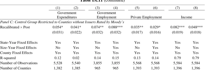
We also perform a series of robustness tests to guarantee that the results are not driven by a lack of comparability between treatment and control groups. Table IA.11 presents the results when we restrict the sample to counties that have at least two issuers (Panel A) and when we exclude counties below the 20th percentile of the amount of bonds issued (Panel B). These tests guarantee that our results are not driven by counties with a small exposure to the municipal bond market and may not be a good control group for our treatment counties. Panel C of Table IA.11 presents the results when we restrict the control group to counties without issuers rated by Moody’s (i.e., counties where all issuers are rated by S&P or Fitch), which mitigates concerns that our results are driven by a Moody’s ex-ante selection of counties based on their creditworthiness. Finally, Figure IA.4 shows that there are no significant differential effects in the house price index of the treatment and control groups before or after the ratings recalibration.
28
Thus, there is no evidence that the 2007-2009 financial crisis had a differential effect on treatment and control groups or that the treatment group recovered faster than the control group from the crisis.
Table IA.12 shows the results using the sample of all counties for which we are able to obtain data on economic outcomes, which comprises more than 90% of the counties in the United States. In this sample, the control group also includes counties without exposure to the municipal bond market (i.e., counties where local governments did not issue bonds in the municipal bond market in the four-year period before the recalibration). The estimates are similar in magnitude and statistically significant.
5. Fiscal Multipliers
Our results support a positive relation between municipal bond rating upgrades and bond financing, government expenditures and employment, private employment, and income. To interpret the magnitude of the results, we estimate local fiscal multipliers for employment (i.e., the increase in jobs from a marginal million dollars in government spending) and income (i.e., the dollar change in income produced by a one-dollar change in government spending). These multipliers are interpreted as the impact of local policy interventions that include direct impacts of government spending (e.g., purchases or hires), as well as impacts through indirect channels (e.g., economic activity created by additional government spending).
We use instrumental variables methods to estimate the fiscal multipliers. We instrument for local government expenditures at the county level using the exogenous variation due to Moody’s 2010 recalibration. The instrument is the interaction variable Recalibrated × Post. We estimate the effect of government spending on government employment, private employment, and income using two-stage least squares in the 2007–2013 county-year panel with county, state-year, and, in some specifications, county-size decile-by-year fixed effects.
Table 10 presents the instrumental variables estimates. Panel A shows results using the sample of bond issuers, and Panel B shows results using the sample of urban counties. The
first-29
stage regressions are similar to columns (1) and (2) of Panel A of Table 5. F-statistics are above 10 in the sample of urban counties in Panel B, but they are usually below 10 in the sample of bond issuers in Panel A. For this reason, we use the estimates in Panel B for the sample of urban counties to generate our estimates of the fiscal multiplier.
The dependent variables are the logarithm of government employment, private employment, and income, so the estimated coefficients are elasticities and must be transformed to recover fiscal multipliers. Per the definition of the elasticity, we multiply the coefficient in each regression by the ratio of government employment, private employment, or income to local government expenditures evaluated at the mean of the data. Following the literature, we estimate the multipliers using the increase in government spending instead of the increase in bond financing.
The creation of local government jobs is calculated as the product of the estimate in column (1) of Table 10, Panel B, by the average ratio of local government employment to government spending by county. The estimates indicate that a marginal million dollars in local government spending results in 6 jobs (= 0.963 6.0) in the local government sector.
The elasticity in column (3) of Table 10 can be translated into the corresponding increase in private sector jobs by multiplying it by the average ratio of private employment to government spending. The results indicate that a marginal million dollars in local government spending results in 45 jobs (= 0.440 102.7 in the private sector). Overall, our results suggest that $1 million in spending increases total employment (local government and private) by 51 jobs (= 6 + 45), which corresponds to a cost per job created of $20,000 (the inverse of the local employment multiplier).
The marginal increase in income is obtained as the product of the estimate in column (5) by the average ratio of income to government spending by county. This implies that government spending has a local income multiplier of 1.9 (= 0.326 5.8). Combining the income and employment multipliers, we estimate that the jobs created have a remuneration of 1.9 × $20,000 = $38,000.