0
A Work Project, presented as part of the requirements for the Award of a Master Degree in Finance from the NOVA - School of Business and Economics
Nova Student Portfolio: Enhancing Performance Through Different Investment Styles
PEDRO HENRIQUE ABREU PARENTE DE MELLO - 34072
A Project carried out on the Master in Finance Program, under the supervision of: Professor Gonçalo Sommer Ribeiro
1
ABSTRACT
This paper tried to build a strategy that beats the S&P 500 using its constituents, when incorporating moving average crossover on sectors as well as using value and growth factors to pick stocks, using weekly rebalancing. Moreover, this strategy was implemented in a portfolio composed by 40% Equity and 60% Bonds and tested with transaction costs (even though its realistic as the NSP does not pay fees). Finally, the results show that a long-portfolio of 40 stocks on S&P 500 equities, with a weekly holding period, presents only satisfactory results for certain types of investors.
Keywords: Asset allocation; Growth investing; Momentum investing; Value investing
This work used infrastructure and resources funded by Fundação para a Ciência e a Tecnologia (UID/ECO/00124/2013, UID/ECO/00124/2019 and Social Sciences DataLab, Project 22209), POR Lisboa (LISBOA-01-0145-FEDER-007722 and Social Sciences DataLab, Project 22209) and POR Norte (Social Sciences DataLab, Project 22209).
2
I. Introduction
The Nova Student Portfolio (NSP) is a course at NOVA - School of Business and Economics, sponsored by a Portuguese investment bank, where each year a group of students from the Nova Masters in Finance actively manage a long only portfolio of stocks and bonds, with an inception Net Asset Value (NAV), in November 2014, of 310,000 USD, under the supervision of two instructors. The participants are required to decide on the most suitable investment strategy to apply, do macroeconomic research, pick stocks, and analyze securities in order to make the best allocation method.
Through the course, the students take turns in seven positions: Investor Relations, Risk Manager, Macro Bull, Macro Bear, Portfolio Manager, Stock Picker and Trader. The Investor Relations is responsible to close the factsheet of the fund, calculate the Unit Participation and write the Investment Committee (IC) minutes; the Risk Manager role is to check if the trades of the week were made, control the Value at Risk (VaR) and volatility of the portfolio and write the risk report; the Macro Bull and Macro Bear present the main events and indicators of the recent past and following periods in order to give information for the IC decide the best allocation method for the portfolio; the Portfolio Manager controls the performance of the fund, checks which style and allocation method performed better over the previous period, ensures diversification within styles and sectors, while performing backtests and suggesting alternative portfolio allocations and/or strategies; the Stock Picker duty is to search and propose potential investments that outperform the benchmark and to set its stop-loss and target price; Finally, the Trader is responsible to execute all the trades, as well as to introduce the stop-loss and target price orders for each security selected to compose the portfolio. Every weekly IC meeting, a student is assigned to one of those functions and briefly gives an overview from his area, based on his role throughout the week, so that the portfolio is closely monitored and often updated in order to enhance the performance. The student’s main objective is to generate the maximum
3
competitive risk-adjusted returns for the NSP portfolio with a low/medium risk profile restriction. The requirements that the portfolio must comply with, in terms of risk, are: not to exceed an annual volatility of 7.00% and a daily VaR of 1.50%. The asset allocation starts with a 40.00% equity and 60.00% bond structure, which corresponds to the benchmark structure, and remains the same, unless decided otherwise by the IC, changing the weights on a maximum of 10% up or down or to risk parity, depending on whether students are more bullish or bearish on the market. Regarding the investments products, positions can be taken in cash stocks, bonds, ETFs, and futures contracts.
The NSP fund began on 13/11/2014 and its performance is measured until 03/05/2019 (end date of class 2018/2019). Over this period, the portfolio presented an annualized return of 4.69% as of 03/05/2019 and an annualized volatility of 7.46%. Moreover, the maximum and minimum weekly returns since the beginning were 3.01% and -3.51%, respectively, while presenting a maximum drawdown of 5.35% and an Info Sharpe1 of 0,63 as Appendix 1 shows. Throughout the 20 ICs in the 2018/2019 year, the portfolio started with a NAV of 355.914,53 USD and obtained a 6.77% total return, thus finishing at 03/05/2019 with 380.026,55 USD and an annualized volatility of 9,26%. When you compare the NSP with the benchmark2, it underperformed by 27bps, with the benchmark presenting a return of 7.04%, increasing the portfolio value by 24.986,67 USD and an annualized volatility of 10.52%. In Appendix 2 it is possible to see the overall performance of the NSP fund and compare it with the benchmark.
During the 2018/2019 period 37 stocks were picked and their average returns outperformed 1,1% more than the S&P500 (our benchmark), thus contributing positively for the performance of the whole portfolio by 2.8%. The stock picks presented more positive returns than the S&P
1 Info Sharpe = Annualized return / Annualized standard deviation
4
500 25 times out of 37, presenting a success rate of almost 70%. Each stock individual performance can be seen in Appendix 3.
The purpose of this project is to help students from following years of the Nova Student Portfolio (NSP) course to have more stock-picking tools in order to enhance the future performance of the fund. In order to achieve quantitative information, to be used to pick stocks, we will use a set of criteria from the available literature. New stock-picking models based on these studies will be created using some of its metrics and a scorecard will be built to rank the stocks, assembling an equity portfolio. The equity part of the portfolio will then be constituted by stocks selected through this best performing model. After, we will use this equity portfolio and test this strategy in a new portfolio, this time composed of 40% equity and 60% bonds. Both the equity strategy and the tested portfolio will, through backtests of thirteen years (2007-2019), be compared with its benchmarks3, to conclude on the research quality. To best understand this paper, it is good to understand that the main point of this project are equities and its different stock-picking possibilities, anchoring on financial information that one may obtain higher returns than the compared benchmark.
II. Literature Review
The Modern Portfolio Theory developed by Markowitz (1952) introduces the idea that portfolios with multiple assets can be constructed by investors in order to maximize returns for a given level of risk. For a given level of expected return, investors can construct portfolios with the lowest risk possible. Aligning variance and correlation, individual securities’ return is less important than how the securities relate with the whole portfolio. Diversification relates with the previous concept mentioned, as it mix a wide variety of securities and investments in
3 Benchmark of the equity strategy: S&P 500 index; Benchmark for the tested portfolio: 40% SPDR S&P 500 ETF Trust + 60% iShares 3-7 Year Treasury Bond ETF.
5
order to reduce portfolio standard deviation and correlation without reducing portfolio mean return. The rationale behind this technique is that a portfolio constructed with different kinds of assets will, on average, decrease the volatility of the portfolio and, at the same time, increase its Sharpe ratio. In theory, if two inversely correlated stocks formed an equal-weighted portfolio, the bad year of one asset would be offset by a good year from the other asset, thus resulting in a portfolio with low volatility. In reality this is not quite simple, there are more than two assets and the returns are less predictable and not perfectly negatively correlated with each other, although this concept still works in reality. Diversifying, in the end, does not eliminate entirely the volatility, but reduces it. Statman (1987) demonstrated by diversifying a portfolio with securities that it is possible to reduce the average standard deviation of annual portfolio returns from 49.24% with one stock in the portfolio up to 19.16% with a portfolio with infinite stocks. That is more than halving volatility.
Financial markets are highly competitive because they are composed by many investors that are informed and knowledgeable, with advantageous compensation schemes to study the market, buy and sell under and over-valued securities. With more participants and the fast dissemination of information, mostly due to the technology revolution, the more likely efficient a market should be. The Efficient Market Hypothesis (EMH) is an investment theory, whereby in an active market with well-informed and intelligent investors, share prices will reflect all the information available, thus being impossible for investors to obtain above average returns and generate a consistent alpha. According to this hypothesis, in an efficient market neither the technical analysis, nor even the fundamentalist analysis, would allow an investor to produce risk-adjusted excess returns, or alpha, consistently as studies made by Fama (1970 and 1998)
show. On the other hand, Rosenberg, Reid and Lanstein (1984), Basu
(1977) and Marshall et al. (2008) proved that the market is not totally efficient. Their trading strategies exposed that even though information is available, it is still possible to benefit from
6
the inefficiency and profit from it. Additionally, some investment styles below will also demonstrate that the market is not efficient.
In Portfolio Management there are different kinds of approaches in order to select securities to invest. Momentum strategy is an investment style that wants to benefit from the market trends, so one can group technical indicators that dictates market entry and exit points for securities, staying invested in it as long as their trend is positive. The pioneer of this strategy is uncertain, but Richard Driehaus considered as the father of the strategy according to Hong and Satchell (2012). On the other hand, a study by Fama and French (2008) already cited a previous work done on this subject by Jegadeesh and Titman (1993). The two discovered a strategy that buying selects stocks based on their past 6-month returns, while holding them for next 6 months, would generate 12.01% compounded excess return on average over the 1965 to 1989 period.
Another example of a momentum strategy is using moving average crossover. One can use a short-term moving average and a long-term moving average as a trading signal. Suppose you use 30-day moving averages and 200-day moving averages for trading signals. One will use the 30-day moving averages as a short-term moving average and the 200-day moving averages as a long-term moving average. When the short-term moving average becomes higher than the long-term moving average it creates a buy signal, while the reciprocal is also true. Anghel (2013) used the technique above in the Bucharest Stock Exchange and managed to obtain indications of geometric excess return adjusted to trading cost and downside risk, while Gurrib (2016) outperformed a buy and hold strategy with the same method applied in the S&P 500 Index, obtaining a higher Sharpe performance between 1993 and 2014 in two different studies.
Value Investing, the second investment style used in this paper, is an investment method developed by Graham et al. (1934) that pick equities which are being priced below their intrinsic value using fundamental ratios and key metrics. This strategy rationale focusses its attention on
7
digging for investments that are undervalued by the market, buying when it is cheap and making profit at the time the stocks reaches its true (intrinsic/fundamental) value and is sold. Jaffe, Keim and Westerfield (1989) improved previous studies from this investment style, more specifically about price earnings ratio (PE), for different time periods and managed to generate returns in distinct periods. On the other hand, Salgueiro (2007) presented a different approach and adopted both of Benjamin Graham and Warren Buffett investment statement in the Brazilian stock market. He obtained average results above the market using some value ratios such as Debt / Total Assets, EBITDA Margin, and Return on Equity (ROE). Again, the previously work cited from Rosenberg, Reid and Lanstein (1984) is relevant for this subject as they developed a trading strategy built on the price to book ratio (PB) for value investors, which yielded positive returns over time. All in all, these studies demonstrate that value ratios provide useful mechanism to discover the intrinsic value of a stock in order to obtain positive returns for compensated risk.
While value investing care about the current intrinsic value of assets, Growth investing proclaims that investment should be made in companies where they can obtain future capital gains when compared to their industry peers or the overall market. Metrics are compared with its previous results, measuring sales or earnings growth, and investments are made if growth is positive, with the expectation that these business growth metrics will continue to improve in the future. Damodaran (2002 and 2008), who is credited to be the father of fundamental investing, presents extended studies related to growth analysis. In his investigations he traced that investment in new assets, defined by him as sustainable growth, and improved efficiency from the current ones, the efficiency growth, creates high returns in the long run period. Corroborating with him, the study from Cooper et al. (2008) discovered that firm's annual asset growth rate is as an economically and statistically good predictor of stock returns. Low asset growth rates companies obtained, on average, 9.1% annualized risk‐adjusted return, while firms
8
with high asset growth rates obtained 10.4% return. Furthermore, Jegadeesh (2002) revealed in his research that after a company reports higher revenues in its quarterly financial results, obtaining revenue growth, its stock price tends to obtain positive abnormal returns.
III. Data and Methodology
The strategy proposed in this project consists in outperform the S&P 500 Index with stock picking based in different investment styles and beat the NSP benchmark by maintaining the 60% bond part of the portfolio invested just as the benchmark, meaning to invest in the iShares 3-7 Year Treasury Bond ETF, while achieving outperformance also with the equities part. Using the sector rotation based on momentum we will select stocks within those sectors based in their value and growth ratios and rebalance the strategy on a weekly basis. If the amount of sectors selected does not fulfil the criteria, we will invest the remaining part, or the total 40% from the equity part of the portfolio, in the SPDR S&P 500 ETF Trust, which is the ETF that represents the equity part of the NSP benchmark. These outcomes will be observed through backtests in a period of thirteen years, from 2007 to 2019, considering high and low markets that will show if the returns are higher or not. Since the average number of stocks presented each year in the NSP portfolio is 40, this is the maximum number of stocks allowed in model. As we want to optimize the portfolio, while also standardizing the number of stocks and sectors tested, the product between the number of sectors and stocks must be 40, thus only allowing only the combinations presented in Table 1.
Table 1. Combinations between the sectors and the number of stocks used in the model
Number of Sectors: Number of Stocks per Sector:
1 40 2 20 4 10 5 8 8 5 10 4
9
As the NSP fund benchmark uses an ETF that replicates and tracks the S&P 500 index, the stocks used in the strategy will also be stocks that composed the S&P 500 index. To do so, we first accessed the Wharton Research Data Services (WRDS) and extracted a list of all the stock that constituted the S&P 500 index from January 2007 to May 2019 with their entry and exit dates from the index. The interval selected was to match the exact same time of the inception of the iShares 3-7 Year Treasury Bond ETF and the end of the 2018/2019 NSP class. The reason to select all the stocks that composed the index through the period and its respective dates is to avoid the survivorship bias.
The survivorship bias applying to this project would mean that we would do back tests of market performance and stock picking based in the current index members of the S&P 500 index, rather than actual constituents over time. Gilbert and Strugnell (2010) tested the effects of survivorship bias based on two other works. The two updated the previous studies using an extended the analyzed period for further 21 months, quantifying the survivorship impact of all those stocks with the current listed stocks on the Johannesburg Stock Exchange (JSE). Gilbert and Strugnell confirmed that the portfolio with the currently listed companies provided higher returns when compared with the returns on portfolios selected from all shares, proving than the existence of survivorship bias. Elton et al. (1996) also found evidences of survivorship in mutual funds and the impact of this on investor return.
To establish the sectors the Global Industry Classification Standard (GICS) classification, developed by S&P Dow Jones Indices (a division from the S&P Global Company), was used as we are analyzing stocks that are members of an index that was also developed by this group (S&P 500). The GICS structure consists of 11 Sectors: Communication Services, Consumer Discretionary, Consumer Staples, Energy, Financials, Health Care, Industrials, Information Technology, Materials, Real Estate, and Utilities.
10
Having retrieved the list of stocks that composed the index and their respective sectors, we accessed a Bloomberg platform to extract all the data used for this analysis. The information extracted from Bloomberg was greater than the period of the analysis, since January 2006, because it is necessary to lag quarterly data to avoid the forward looking bias as Bloomberg reports data ahead of the release date and to incorporate the moving averages studies. With this sample, we excluded from the database all the stocks that have not returned any closing price, as it would not be able to calculate their returns for the strategy. This left the sample with 751 unique stocks. If a company composed more than one time the index, it was considered as a different observation, thus retrieving again all its data as it was a new stock. In the end, the sample accounted with 767 observations.
Momentum crossover applied to sector is the tendency to benefit from the market trends with factors that indicates market entry and exit points for sectors based on well performing sectors. Eakins and Stansell (2004) and O'Neal (2000) reported that momentum strategies applied to sectors provided higher risk-adjusted returns. To study and define which sectors to invest, a model will be made with two signals. Once the model incorporates both signals, this sector is selected to be invested and another methodology used, that will be explained later, is going to choose the stocks from the sectors to be invested.
The 1st signal of the strategy consist in defining a short-term moving average (STMA), a long-term moving average (LTMA) and generating a signal out of this information set. Table 2 presents the moving averages tested.
Table 2. Moving Averages used in the Signals for the momentum metrics
Moving Average 5 Day Moving Average 10 Day Moving Average 20 Day Moving Average 30 Day Moving Average 50 Day Moving Average 100 Day Moving Average 200 Day
11
A binary signal system was given to distinguish if the STMA was bigger than the LTMA. If this was true the number 1 was given to the sector, otherwise the number 0.
The 2nd signal for the strategy consists in measure how strong is the difference between the STMA and the LTMA and select the sectors with strongest momentum. To do so, we divided for each sector the value of the STMA by the value of the LTMA selected. After this, the eleven sectors were ranked from highest to lowest values and again a binary signal system was given, attributing the number 1 to the highest momentum sectors which incorporated both signals, depending on the number of sectors tested, and 0 for the remainders.
The trigger to select the sector is made when the binary results from the two signals is 1. Table 3 shows the overall binary systems adopted.
Table 3. Overall Binary System used to select the sectors
1st Signal: If Short-Term Moving Average > Long-Term Moving Average = 1; 0 otherwise 2nd Signal: If is top strong sector momentum = 1; 0 otherwise
If both 1st Signal and 2nd Signal = 1, then invest in the sector, otherwise no
Based on the strategy from Greenblatt (2006)4 that picked stocks using only two indicators and obtained superior returns with lower risk, when compared with the market between 1988 and 2004, this model will also use two metrics to select stocks – a growth and a value metric. It will consist in selecting stocks that presents the highest ratios of its corresponding sector. The series of value and growth metrics presented in Table 4 will be tested in order to pick the stocks. These ratios were selected based on previous studies cited in this work that presented relevant results.
Table 4. Value and Growth Metrics tested to select stocks Value Metrics Growth Metrics
Price Earnings Ratio Revenue - 1 Year Growth Price to Book Ratio Net Income - 1 Year Growth
12
Return on Equity Assets - 1 Year Growth EBITDA Margin EBITDA - 1 Year Growth
To analyze the quarterly data, first the stocks were divided based on each sector retrieved from Bloomberg. Following this, we lagged all the quarterly data used in this model. An input was created to check if lagging data for longer periods would provide better results and also to avoid the forward looking bias previous explained. The lag selected will retrieve the data from the previous number of weeks based on Table 5 and it starts already with a 3 months lag because results are quarterly.
Table 5. Lagged data tested in the model
Number of Months Lagged: Number of Previous Weeks the Lagged Data Corresponds to:
3 12
6 24
9 36
12 48
The series of quarterly results displayed on a weekly basis will show for each company only if the date of that company is between the start and end date interval of its membership on the S&P 500 index. If the stock did have not presented quarterly results or it was out of the membership interval, the cell will be blank in the scorecard. The next process is to pick the stocks. The portfolio will consist in ranked stocks, per sector, from the best metric result to the worst. To compose the final ranking, the positions in each of the two ranks will be summed and then reranked by sector, but this time the ranking will be done from the stocks that obtained the highest value and growth composition to the worst. Finally, a binary signal will be used to assign the number 1 to the best stocks from each sector based on the maximum number of stocks per sector allowed from the previously mentioned Table 1.
Each stock return will be calculated with a formula that enables us to include transaction costs in its weekly returns as the stocks in the portfolio changes. Even though the NSP does not incur in transaction costs, since the fund belongs to the sponsor Bank and the rules of the portfolio
13
do not consider it, a strategy taking in account 0,08% (8 basis points) of transaction costs will also be tested to check if it produces relevant results as it is necessary to compute the influence of the bid-ask spread and some brokerage fees.
The strategy will start at 12/01/2007 since the iShares 3-7 Year Treasury Bond ETF only started to be traded in 11/01/2007. The model will buy the stocks to compose the portfolio at the closing price of the week and will be rebalanced weekly according to the signals from the sectors and the stock positions at the end of the previous week.
To analyze how the stock picks performed, some comparisons will be made with the S&P 500 Index and the NSP benchmark. The main comparisons performance will contrast the overall return of the strategy and the Info-Sharpe, which the formula (1) is presented below.
𝐼𝑛𝑓𝑜 − 𝑆ℎ𝑎𝑟𝑝𝑒 = 𝐴𝑣𝑒𝑟𝑎𝑔𝑒 𝐴𝑛𝑛𝑢𝑎𝑙 𝑅𝑒𝑡𝑢𝑟𝑛
𝐴𝑣𝑒𝑟𝑎𝑔𝑒 𝐴𝑛𝑛𝑢𝑎𝑙𝑖𝑧𝑒𝑑 𝑉𝑜𝑙𝑎𝑡𝑖𝑙𝑖𝑡𝑦 (1)
To control the portfolio, some risk management metrics will be used. A back test to control the VaR with a confidence interval of 99%, an annual target volatility of 7% and a daily VaR limit of 1,5% ( or a 3,4% weekly VaR limit) will be made and also a drawdown analysis comparing the stock picking strategy with the S&P 500.
Finally, we will only consider for comparison the mix of metrics that obtained the highest overall return and Info-Sharpe
IV. Results
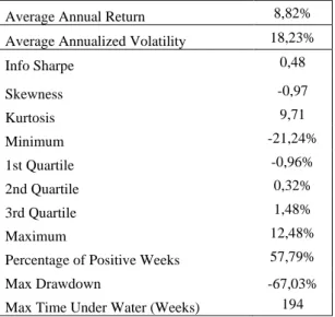
This part presents the performance results of the equity strategy and the portfolio built against the S&P 500 and the NSP benchmark between the period of 2007 to 2019 and concludes about the excess return generated. The focus will be mainly in the results from the best strategy achieved. Table 6 below illustrates the descriptive statistic from the equity strategy portfolio
14
obtained with the EBITDA Margin and the EBITDA 1-year growth ratio, the best combination of one Value ratio and one Growth ratio.
Table 6. Descriptive statistics for the Equity Strategy built
Average Annual Return 8,82% Average Annualized Volatility 18,23% Info Sharpe 0,48 Skewness -0,97 Kurtosis 9,71 Minimum -21,24% 1st Quartile -0,96% 2nd Quartile 0,32% 3rd Quartile 1,48% Maximum 12,48%
Percentage of Positive Weeks 57,79% Max Drawdown -67,03% Max Time Under Water (Weeks) 194
The portfolio, which is composed with the stocks that present the best ratios of its corresponding sector from the S&P 500 Index, obtained an Info Sharpe of 0.48 with a 3-month lag on their fundamental data. In Appendix 4 it is possible to see a comparison between the cumulative returns from this equity strategy and the S&P 500 constituents. Appendix 5 and 6 presents more information regarding monthly returns, as well as annual returns. Over the thirteen years analyzed, this tactic obtained 57.79% of excess return, suggesting that the model has some significant evidence of outperformance if others want to adopt the model. The overall return from this equity strategy was 108.91%, or an average annual return of 8.82%. If the amount of 370.000 USD were invested at this strategy since its inception, (12/01/2007), the total amount in 03/05/2019 would be 772,965.55 USD. The negative side from this strategy is the higher drawdown it presents when you compare it to the S&P 500 Index ( -67.03% vs -56.24% maximum drawdown to the Index), which was reached during the worst time in this backtest, the financial crisis that happened in the United States of America in 2007-2008, but the maximum number of weeks under water was smaller than the index as it is possible to see in
15
Appendix 7. The strategy also presents a level of kurtosis of 9,71, being a high number when compared with the kurtosis of 3 presented in the normal distribution. This excessive number indicates that it has a higher probability to obtain extreme positive and negative results from the event when compared with the probability from the normal distribution, thus indicating the presence of fat tails. Additionally, the best strategy displays a negative skewed distribution from its results, indicating that the returns distribution are more frequently presented on the right side. This indicates that the probability of abnormal positive returns is higher.
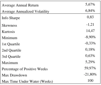
The second test consisted in creating a portfolio made from 40% equity and 60% bonds. The 40% equity was represented by the best equity strategy obtained, the EBITDA Margin and the EBITDA 1-year growth ratio, and the 60% bond part of the portfolio with the iShares 3-7 Year Treasury Bond ETF was incorporated in the total allocation method. The descriptive statistics are displayed in Table 7 below.
Table 7. Descriptive statistics for the tested portfolio
Average Annual Return 5,67% Average Annualized Volatility 6,84%
Info Sharpe 0,83 Skewness -1,21 Kurtosis 14,47 Minimum -8,90% 1st Quartile -0,33% 2nd Quartile 0,18% 3rd Quartile 0,63% Maximum 5,29%
Percentage of Positive Weeks 59,97% Max Drawdown -21,80% Max Time Under Water (Weeks) 100
The portfolio mixing equities and bonds obtained an Info-Sharpe of 0.83 and the maximum drawdown between the 2007-2019 period of -21.80%, obtaining superior returns than the benchmark, when you consider the return adjusted for the risk and total return from the strategies. In Appendix 8 it is possible to see the descriptive statistics for the benchmark for
16
comparison. Additionally, the cumulative returns for both the portfolio strategy and the benchmark can be found in Appendix 9, while looking at Appendix 10 one can see the drawdown. Appendix 11 and Appendix 12 show the monthly and annual returns for each portfolio. The percentage of positive weeks displayed and the maximum drawdown presented this time show slightly worst numbers than the NSP benchmark (100 weeks under water for the portfolio strategy against 98 weeks under water for the benchmark and -21.80% maximum drawdown versus -21.76% again for the benchmark). Even though, the portfolio strategy obtained more percentage of positive weeks than the equity strategy. The portfolio also yielded an average annual return 0.39p.p higher than the benchmark, while also obtaining higher skewness and lower kurtosis.
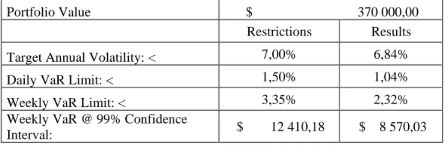
Concerning the historical VaR for this portfolio, Table 8 presents the descriptive calculated based on the NSP investment policy for 2018/2019. Appendix 13 also illustrates the historical distribution of returns for this portfolio with an initial capital of 370,000 USD. With a 99% confidence interval, this portfolio won’t lose more than 8,570.03 USD, 99 out of 100 times. According to these statistics, this portfolio is valid and can be used by the NSP students in order to pick stocks to compose the portfolio.
Table 8. Descriptive statistics for historical VaR applied to the tested portfolio
Portfolio Value $ 370 000,00 Restrictions Results Target Annual Volatility: < 7,00% 6,84% Daily VaR Limit: < 1,50% 1,04% Weekly VaR Limit: < 3,35% 2,32% Weekly VaR @ 99% Confidence
Interval: $ 12 410,18 $ 8 570,03
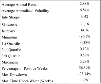
Table 9 presents the statistics for the 40% equity strategy obtained and the 60% iShares 3-7 Year Treasury Bond ETF simulating the study with the inclusion of 0,08% transaction cost to the portfolio, replicating the results for an investor who has trading costs. Appendix 14 presents
17
the cumulative return of both strategies. The introduction of transaction costs sharply decreased the cumulative return of the strategy, as expected. This result is due to the weekly rebalancing of the portfolio, which yield lower returns as the transaction costs decrease the portfolio returns. In the end, comparing with the NSP benchmark, this strategy is not attractive for an investor who has trading costs as he would obtain higher returns investing in the benchmark.
Table 9. Descriptive statistics for the tested portfolio considering transaction costs
Average Annual Return 2,88% Average Annualized Volatility 6,84%
Info Sharpe 0,42 Skewness -1,16 Kurtosis 14,36 Minimum -8,91% 1st Quartile -0,38% 2nd Quartile 0,12% 3rd Quartile 0,59% Maximum 5,29%
Percentage of Positive Weeks 56,39% Max Drawdown -23,14% Max Time Under Water (Weeks) 128
Based on the results presented during this section and on Table 10 below, one should be aware that using value and growth ratios in a model using crossover moving averages in sectors momentum improves the risk-adjusted return and the relative performance compared with the benchmark,. Beating the benchmark 8 out of 13 years and underperforming only one time more than 0.13%, it statistically proved that this strategy overperformed the benchmark and yielded higher return.
Table 10. Ranking of Models based on their Info-Sharpe Model Info-Sharpe
Tested Portfolio 0,83 Benchmark 0,79 Equity Strategy 0,48 S&P 500 0,33
18
V. Summary and Conclusion
In this paper a stock picking method was proposed with the intention to create a strategy that outperforms the benchmark in the based on momentum, value and growth investment styles. Two models overall were tested with this strategy, one without and another including transaction costs, through a period of thirteen years comprehending bull and bear markets for backtests to be orchestrated. In addition, a risk management assessment was made to verify if the strategy complies with the NSP investment policy and could be used by NSP students.
This project revealed that the use of different investment styles for stock picking strategy enhanced results and increased the Info-Sharpe, while getting very similar values of skewness with the benchmark for the sample considered. Besides that, the strategy does not exceed the risk parameters, being suitable for use by the Nova Student Portfolio students. On the other hand, when it comes to investors that incur in transactions costs such as brokerage fees and bid-ask spreads, to name a few, the stock picking strategy was not as attractive as investing in ETFs thattracks underlying indexes.
Finally, the outcomes achieved in this paper represents a simple combination of one value and one growth ratio to achieve a final rank. For this reason, it would be fascinating to consider more ratios of each investment style in order to pick the stocks, different rebalancing periods, as well as different moving averages in future studies. Moreover, not only a regression and a correlation between the EBITDA Margin and the EBITDA 1-Year growth obtained as the best ratios could be tested in order to understand how these ratios relate, but also a test for weight optimization could be tested to check if it is possible to obtain even higher returns than this study.
19
VI. Bibliography
Anghel, D. (2013). “How reliable is the moving average crossover rule for an investor on the Romanian stock market?”. The Review of Finance and Banking, 5(2).
Rosenberg, B., Reid K., & Lanstein R. (1984). Persuasive evidence of market inefficiency. Journal of portfolio management, 11, 9-17.
Basu, S. (1977). “Investment performance of common stocks in relation to their price‐earnings ratios: A test of the efficient market hypothesis”. The journal of Finance, 32(3), 663-682. Cooper, M. J., Gulen, H., & Schill, M. J. (2008). Asset growth and the cross‐section of stock returns. The Journal of Finance, 63(4), 1609-1651.
Damodaran, A. (2002). Estimating Growth. Investment Valuation. 2nd Edition//pages. stern. nyu. edu, 6.
Damodaran, A. (2008). The origins of growth: past growth, predicted growth and fundamental growth. Predicted Growth and Fundamental Growth (June 14, 2008).
Eakins, S. G., & Stansell, S. R. (2004). “Do Momentum Strategies Work?”. The Journal of Investing, 13(3), 65-71.
Elton, Edwin J., Gruber, Martin J., Blake, Christopher R., (1996). Survivor Bias and Mutual Fund Performance, The Review of Financial Studies, Volume 9, Issue 4, Pages 1097– 1120
Fama, E., (1970). “Efficient capital markets: a review of theory and empirical work”. Journal of Finance 25, 383-417.
Fama, E., (1998). “Market Efficiency, Long-Term Returns, and Behavioral Finance”. Journal of Financial Economics 49 (3): 283–306.
Fama, E. F., & French, K. R. (2008). “Dissecting anomalies”. The Journal of Finance, 63(4), 1653-1678.
Gilbert, E. & Strugnell, D., (2010). “Does survivorship bias really matter? An empirical investigation into its effects on the mean reversion of share returns on the JSE (1984–2007)”. Investment Analysts Journal, 39:72, 31-42
20
Graham, B., Dodd, D. L. F., & Cottle, S. (1934). Security analysis (pp. 44-45). New York: McGraw-Hill.
Greenblatt, J. (2010). The Little Book That Beats the Market (Vol. 9). John Wiley & Sons. Gurrib, I. (2016). Optimization of the double crossover strategy for the S&P500 market index. Optimization, 7(1).
Gurrib, I. (2016). The Moving Average Crossover Strategy: Does It Work for the S&P500 Market Index?.
Gurrib, I. (2016). “Optimization of the Double Crossover Strategy for the S&P500 Market Index”. Global Review of Accounting and Finance, 7(1), 92-107.
Hong, K. J., & Satchell, S. (2012). “Defining single asset price momentum in terms of a stochastic process”. Theoretical Economics Letters, 2(03), 274.
Jaffe, J., Keim, D. B., & Westerfield, R. (1989). “Earnings yields, market values, and stock returns”. The Journal of Finance, 44(1), 135-148.
Jegadeesh, N. (2002). Revenue growth and stock returns.
Jegadeesh, N., & Titman, S. (1993). “Returns to buying winners and selling losers: Implications for stock market efficiency”. The Journal of finance, 48(1), 65-91. Markowitz, Harry. (1952). Portfolio Selection. The Journal of Finance 7 (1): 77–91.
Marshall, B., Treepongkaruna, S., & Young, M. (2008). “Exploitable arbitrage opportunities exist in the foreign exchange market”. In American Finance Association Annual Meeting, New Orleans.
O'Neal, E. S. (2000). “Industry momentum and sector mutual funds”. Financial Analysts Journal, 56(4), 37-49.
Salgueiro, G. C. (2007). Comparação das filosofias de investimento de Benjamin Graham e Warren Buffett: aplicação no mercado brasileiro. São Paulo: Universidade de São Paulo. Statman, M. (1987). “How Many Stocks Make a Diversified Portfolio?”. Journal of Financial and Quantitative Analysis, 22(3), 353-363
21
VII. Appendix
Appendix 1. Nova Student Portfolio performance statistics since inception
UP 122.58 Annualized Return 4.69% Annualized Volatility 7.46% Info-Sharpe 0.63 Skewess (weekly) -0.62 Kurtosis (weekly) 2.09 Max Return (weekly) 3.01% Min Return (weekly) -3.51% Max Drawdown -5.35%
22
Appendix 3. NSP stock picks performance in 2018/2019
Appendix 4. Cumulative Return comparison between the Equity Strategy and S&P500 Name Ticker %share Return of the pick Return of the Spy Difference
NIO INC - ADR NIO US Equity 1,1% 27,5% 4,6% 22,9%
ROYAL CARIBBEAN RCL US Equity 2,3% 25,1% 9,1% 16,0%
ALIBABA GRP-ADR BABA US Equity 2,3% 21,4% 6,9% 14,6%
ADOBE INC ADBE US Equity 2,4% 26,2% 12,9% 13,3%
MICRON TECH MU US Equity 2,3% 19,2% 6,6% 12,6%
AMERIPRISE FINAN AMP US Equity 2,3% 22,9% 11,8% 11,1%
ROYAL BANK OF CA RY US Equity 2,3% 13,5% 5,8% 7,7%
JAZZ PHARMACEUTI JAZZ US Equity 1,2% 4,0% -3,6% 7,6%
WALT DISNEY CO DIS US Equity 2,3% 16,7% 9,5% 7,3%
EMERG MKT INT EC EMQQ US Equity 2,3% 5,3% -1,2% 6,6%
APPLE INC AAPL US Equity 2,3% 4,4% -1,7% 6,1%
HDFC BANK-ADR HDB US Equity 2,3% 4,7% -1,2% 5,9%
LOCKHEED MARTIN LMT US Equity 2,4% 14,0% 8,5% 5,4%
IAC/INTERACTIVEC IAC US Equity 2,2% 6,9% 1,9% 5,0%
PHILIP MORRIS IN PM US Equity 2,3% 1,1% -3,9% 5,0%
AMERICAN OUTDOOR AOBC US Equity 2,3% 2,5% -1,7% 4,2%
RED HAT INC RHT US Equity 2,3% 0,1% -3,6% 3,6%
ACCENTURE PLC-A ACN US Equity 2,3% 9,2% 5,6% 3,6%
RESTAURANT BRAND QSR US Equity 2,3% 2,3% -1,2% 3,5%
AMERICAN TOWER C AMT US Equity 2,3% -0,1% -3,6% 3,5%
TENCENT HOLD-ADR TCEHY US Equity 2,3% 1,7% -1,7% 3,4%
BANK OF AMERICA BAC US Equity 2,3% 4,5% 1,2% 3,3%
TAPESTRY INC TPR US Equity 2,3% -0,2% -3,4% 3,1%
ISHARES TIPS BON TIP US Equity 20,9% 0,8% 0,0% 0,8%
OMEGA HEALTHCARE OHI US Equity 2,3% -1,1% -1,7% 0,6%
AT&T INC T US Equity 2,3% -4,1% -3,6% -0,5%
NOVO-NORDISK-ADR NVO US Equity 2,3% 5,9% 6,6% -0,7%
ABIOMED INC ABMD US Equity 2,3% -4,4% -1,7% -2,7%
DELTA AIR LI DAL US Equity 2,3% 4,8% 9,1% -4,3%
VISA INC-CLASS A V US Equity 2,3% -8,7% -2,3% -6,4%
METLIFE INC MET US Equity 2,3% -10,9% -3,6% -7,3%
MOLSON COORS-B TAP US Equity 2,3% -2,8% 9,1% -11,9%
ACTIVISION BLIZZ ATVI US Equity 1,2% -11,0% 2,4% -13,4%
GOLDMAN SACHS GP GS US Equity 2,2% -19,7% -5,5% -14,2%
SQUARE INC - A SQ US Equity 2,3% -21,0% -4,2% -16,8%
TESLA INC TSLA US Equity 2,3% -14,0% 4,6% -18,6%
WALGREENS BOOTS WBA US Equity 2,3% -22,6% 8,8% -31,4%
Average 1,3%
Nº of Stocks
Positive/Above S&P 500 Index 25
Negative/Below S&P 500 Index 12
2,8% 1,7% 1,1% Weighted Return of Stock Picks
Weighted Return of SPY (if the same amount was invested in the SPY) Weighted Difference
23
Appendix 5. Equity Strategy Monthly and Annual Returns
Appendix 6. S&P 500 Monthly and Annual Returns
Appendix 7. Drawdown comparison between the Equity Strategy vs the S&P 500
Appendix 8. Descriptive statistics for the NSP benchmark
Average Annual Return 5,29% Average Annualized Volatility 6,73% Info Sharpe 0,79 Skewness -1,43 Kurtosis 17,69 Minimum -9,23% 1st Quartile -0,30% 2007 2008 2009 2010 2011 2012 2013 2014 2015 2016 2017 2018 2019 1 0,62% -11,60% -5,10% -8,97% -1,24% 1,53% 8,56% -1,25% 0,07% -4,71% 4,02% 7,39% 5,84% 2 3,28% 4,14% -11,37% 4,96% 4,87% 4,42% 0,36% 5,04% 1,40% -0,13% -0,72% -2,55% 4,14% 3 -1,46% -2,12% 10,60% 6,15% 1,06% 2,00% 4,43% -1,42% -1,74% 4,22% 0,96% -2,22% 1,16% 4 4,57% 6,31% 6,00% 2,67% 4,29% -0,26% -0,45% -0,07% 1,52% -0,32% 0,55% 0,28% 1,67% 5 -1,88% 1,15% 6,55% -6,78% -1,41% -9,83% 4,08% 3,60% -1,45% 1,42% 2,76% 3,35% 0,43% 6 2,32% -6,02% -0,43% -0,28% -4,02% 3,04% -0,48% 2,84% -0,41% 0,03% 1,70% 0,10% 0,00% 7 -2,05% -6,94% 7,81% 2,16% 5,40% 0,40% 4,63% -0,05% 1,44% 4,07% 0,10% 3,31% 0,00% 8 0,63% 0,99% 4,21% -2,40% -9,54% 0,45% -3,22% 2,05% -4,62% -2,56% -1,60% 3,07% 0,00% 9 4,31% -5,50% 0,37% 7,68% -1,61% 2,13% 5,44% -3,04% -3,61% 0,95% 4,76% 1,08% 0,00% 10 1,43% -20,07% -1,67% 2,65% 10,48% -2,90% 4,20% 2,27% 7,62% -3,24% 2,63% -8,96% 0,00% 11 -3,23% -7,21% 5,28% 1,30% -8,09% 2,06% 4,21% 3,12% 0,44% 8,36% 1,53% 6,56% 0,00% 12 1,76% -2,50% 5,30% 5,53% 8,34% -2,94% 2,60% 1,84% -0,05% 2,03% 4,23% -8,38% 0,00%
Total Annual Return 10,32% -49,37% 27,57% 14,66% 8,51% 0,09% 34,34% 14,91% 0,60% 10,11% 20,93% 3,02% 13,24%
Equity Strategy Monthly Returns
2007 2008 2009 2010 2011 2012 2013 2014 2015 2016 2017 2018 2019 1 -0,60% -10,54% -5,53% -4,78% 1,48% 4,56% 6,92% -3,25% -4,59% -6,04% 2,46% 7,19% 6,95% 2 2,02% 0,00% -11,65% 2,81% 3,35% 3,68% 0,84% 4,22% 5,34% 0,40% 3,12% -4,47% 4,69% 3 -2,11% -1,16% 10,43% 5,47% -0,46% 3,08% 3,47% -0,10% -2,09% 4,41% -0,20% -3,95% 1,48% 4 5,02% 6,09% 5,98% 1,71% 3,72% -0,36% 0,83% 0,31% 2,71% 1,43% 0,91% 1,09% 3,65% 5 1,44% 0,18% 5,93% -8,55% -2,41% -6,29% 3,02% 3,18% -0,49% 1,62% 1,32% 1,91% 0,20% 6 -0,82% -9,11% -0,03% -1,17% -4,82% 3,31% -1,51% 1,93% -0,28% -2,98% 0,31% -0,11% 0,00% 7 -3,00% -1,63% 7,20% 2,28% 1,86% 1,73% 5,18% 0,88% 0,11% 6,47% 1,99% 3,63% 0,00% 8 1,03% 1,97% 4,11% -3,42% -9,36% 1,48% -3,53% 1,26% -5,62% -0,21% -1,18% 2,89% 0,00% 9 3,52% -5,60% 1,49% 7,60% -3,93% 2,39% 3,54% -1,03% -2,94% -0,04% 3,08% 0,43% 0,00% 10 0,56% -22,49% -0,79% 2,97% 12,74% -2,01% 3,94% 1,76% 7,38% -1,95% 2,42% -9,17% 0,00% 11 -3,59% -7,78% 5,20% 0,52% -10,36% 0,30% 2,58% 2,42% 0,52% 4,01% 0,82% 3,75% 0,00% 12 -0,18% -2,65% 3,16% 5,58% 8,19% -0,98% 1,95% 1,02% -1,40% 1,14% 2,70% -10,47% 0,00%
Total Annual Return 3,28% -52,71% 25,51% 11,01% 0,00% 10,90% 27,23% 12,60% -1,34% 8,28% 17,75% -7,29% 16,98%
24
2nd Quartile 0,16% 3rd Quartile 0,57%
Maximum 5,29%
Percentage of Positive Weeks 60,59% Max Drawdown -21,76% Max Time Under Water (Weeks) 98
Appendix 9. Tested Portfolio vs NSP Benchmark cumulative return comparison
Appendix 10. Drawdown comparison between the Tested Portfolio vs NSP Benchmark
Appendix 11. Portfolio Strategy Monthly and Annual Returns
2007 2008 2009 2010 2011 2012 2013 2014 2015 2016 2017 2018 2019 1 0,03% -2,74% -2,95% -2,76% -0,04% 0,86% 3,11% 0,28% 1,67% -0,67% 1,65% 2,37% 2,32% 2 1,98% 2,59% -4,93% 2,22% 1,52% 1,48% 0,28% 2,10% -0,25% 0,25% 0,20% -1,36% 2,06% 3 -0,02% -0,50% 4,94% 1,86% 0,48% 0,49% 2,04% -1,04% -0,38% 1,38% 0,25% -0,57% 1,28% 4 1,90% 0,90% 1,99% 1,75% 2,52% 0,57% 0,13% 0,19% 0,98% 0,26% 0,61% -0,38% 0,61% 5 -1,03% 0,06% 1,96% -1,81% 0,33% -3,66% 0,84% 2,09% -0,91% 0,38% 1,29% 1,60% 0,07% 6 0,95% -2,00% -0,58% 0,64% -0,76% 1,37% -0,98% 1,01% -0,75% 0,95% 0,57% 0,25% 0,00% 7 0,14% -2,79% 3,46% 1,87% 2,51% 0,41% 2,04% -0,09% 1,29% 1,87% 0,28% 1,14% 0,00% 8 1,36% 1,45% 2,06% -0,52% -2,65% 0,42% -1,79% 1,18% -1,78% -1,54% -0,34% 1,64% 0,00% 9 2,01% -1,88% 0,56% 3,50% -0,54% 0,83% 2,86% -1,59% -1,19% 0,67% 1,56% 0,03% 0,00% 10 1,26% -6,88% -0,42% 1,68% 3,79% -1,47% 2,05% 1,55% 3,05% -1,70% 0,89% -3,37% 0,00% 11 0,46% -0,62% 3,13% -0,20% -2,60% 1,25% 1,66% 1,65% -0,07% 2,07% 0,61% 2,94% 0,00% 12 0,69% 0,19% 0,83% 1,11% 3,65% -1,32% 0,26% 0,24% -0,13% 0,80% 1,52% -2,39% 0,00%
Total Annual Return 9,73% -12,20% 10,04% 9,36% 8,19% 1,24% 12,50% 7,58% 1,54% 4,72% 9,10% 1,92% 6,34%
25
Appendix 12. NSP Benchmark Monthly and Annual Returns
Appendix 13. Tested portfolio return distribution
Appendix 14. Tested Portfolio vs NSP Benchmark cumulative return comparison with transaction costs 2007 2008 2009 2010 2011 2012 2013 2014 2015 2016 2017 2018 2019 1 -0,53% -2,17% -2,95% -1,02% 1,08% 2,22% 2,51% -0,47% -0,12% -1,18% 1,01% 2,27% 2,80% 2 1,54% 1,17% -4,93% 1,47% 0,99% 1,23% 0,56% 1,87% 1,38% 0,59% 1,82% -2,03% 2,37% 3 -0,20% -0,15% 4,94% 1,62% -0,08% 0,99% 1,69% -0,47% -0,45% 1,51% -0,13% -1,24% 1,46% 4 2,14% 0,77% 1,99% 1,44% 2,34% 0,55% 0,71% 0,39% 1,51% 1,02% 0,79% 0,02% 1,46% 5 0,30% -0,19% 1,96% -2,41% 0,03% -2,16% 0,51% 2,00% -0,42% 0,56% 0,79% 1,09% -0,01% 6 -0,14% -3,22% -0,48% 0,39% -1,02% 1,56% -1,32% 0,72% -0,64% -0,23% 0,09% 0,26% 0,00% 7 -0,48% -0,66% 3,26% 1,88% 1,13% 1,00% 2,29% 0,32% 0,84% 2,90% 1,08% 1,29% 0,00% 8 1,79% 2,10% 2,18% -0,81% -2,51% 0,95% -1,81% 0,96% -2,12% -0,48% -0,08% 1,66% 0,00% 9 1,80% -2,00% 1,01% 3,51% -1,36% 0,99% 2,14% -0,75% -0,85% 0,31% 0,93% -0,16% 0,00% 10 0,96% -7,71% -0,09% 1,88% 4,72% -1,04% 2,01% 1,39% 3,02% -1,11% 0,86% -3,44% 0,00% 11 0,44% -0,62% 3,27% -0,61% -3,37% 0,65% 1,11% 1,49% 0,06% 0,38% 0,41% 1,85% 0,00% 12 -0,17% 0,19% -0,02% 1,38% 3,60% -0,46% 0,07% -0,03% -0,62% 0,58% 1,01% -3,07% 0,00%
Total Annual Return 7,45% -12,49% 10,13% 8,73% 5,54% 6,46% 10,46% 7,41% 1,59% 4,85% 8,58% -1,51% 8,08%