A Work Project, presented as part of the requirements for the Award of a Master Degree in Finance from the NOVA School of Business and Economics.
Analysts Consensus As an Investment Tool.
Are There Any Prophets?
Roberto Tedesco
ID: 2450
A Project carried out on the Master in Finance Program, under the supervision of:
Abstract
The aim of this research is to test whether analysts recommendations can be used as a
tool in decision making process. To test this hypothesis, five portfolios are built following
the consensus on the constituents of the Standard and Poor‘s 500 Index. I find that the
top-rated stocks do not over-perform the market. Furthermore, the former are beaten, in
terms of risk-adjusted performance, by portfolios based on less recommended stocks. I
find that analysts recommendations follow specific patterns with regards to exposure to
market risk, book-to-market factor and performance momentum. Finally, a trading strategy,
based on the change in the average consensus level is presented. I find that it is possible
to generate positive Sharpe Ratios by extending strategys holding period to a maximum of
three months.
Key Words: Trading Strategy, Analyst Recommendations, Efficient Market Hypothesis, Abnor-mal Returns.
1
Introduction
The aim of this study is to examine whether analysts recommendations have investment value and, therefore, can be used as a tool in decision making. In this regard, the academic theory and finance practitioners are at odds. According to the former, the semi strong-strong form of market efficiency should not allow any investor to profit (in terms of positive excess returns) from information that are publicly available, such as analysts recommendations, as security prices reflects them instantaneously (Malkiel and Fama, 1970).
and investment banks, which issue these recommendations, should be compensated for their search of information they use to rate the investment potential of stocks in the form of under-writing fees or brokerage commission. At the same time, an investor’s incentive to pay for these recommendations is represented by the expectation of large profits.
The motivation of this research is to assess whether the analysts forecasting and stock-picking ability are valuable to investors and, therefore, should be used as a tool in decision making. In general, stock recommendations can be accessed by investors and other interested parties, as these information are generally publicly available. Hence, the buy and sell recom-mendations are likewise much of interest and achieve a large number of market practitioners. In this study, the performance of different portfolios whose components are decided by following the average consensus for each stock in the sample is tested. After, the performances of these portfolios are tested against different factor models. Finally, a trading strategy based on the change in the average level of recommendation for each firm is devised.
2
Review of the Related Literature
A number of previous studies examined how publicly available recommendations affect stock returns and as to whether investors are able to benefit from the analysts’ opinion. Examples include Womack (1996) and Barber and Odean (2001). Some authors have also assessed the role of herding: Welch (2005) and Jegadeesh and Kim (2010).
Barber and Odean (2001) are the first to take a more investor-focused perspective by in-corporating trading costs and by implementing a number of different investment strategies and associated portfolio turnover.
A different approach in analyzing analysts recommendations is given by Desai et al. (2000). The authors evaluate the performance of the picks of individual financial analysts belonging to different investment banks. They find that stocks recommended byThe Wall Street Journal
all-star analysts outperform comparable benchmark stocks of their industry counterparts. As consequence, analysts who are ranked as experts in each one of the industry in the annualWSJ
rankings show superior ability in stock picking.
3
Data
3.1
Data Collection
re-search. The S&P 500’s components, however, are characterized by sufficiently larger coverage than the rest of the American stock market.
As the labels used by security analysts is different among different brokers, the I/B/E/S labeling is used. I/B/E/S assigns a standardized numerical rating scale which goes from 1 (”Strong Buy”) to a maximum of 5 (”Strong Sell”)1. Additionally, assigning a numerical value to the text recommendations enables to calculate the consensus level. Ratings of 6 also also appear for those stocks whose coverage was not initiated yet or dropped by one analyst. Fur-thermore, the I/B/E/S database allows to chose between three possible dates: the Activation Date, the date on which the recommendation was recorded by Thomson Reuters; the Announce Date, which is the date that the recommendation was reported and the Review Date, which is the date on which the most recent recommendation was confirmed by I/B/E/S with the individual contributor. For the sake of this study, only the Announce Date is considered. This decision was made to avoid that discrepancies between the date in which the recommendation was avail-able for the first time and the date in which it was recorded by Thomson Reuters may result in trading opportunities.
Another characteristic of the I/B/E/S database is that the data made available for the down-load do not contain all the recommendations available on the market. This is due to the fact that some brokerage houses disclose their ratings only to paying clients. However, this is a common problem that affects all the research in the filed.
Analysts and brokerage firms contributing to the sample are uniquely identified by a number since they can be observed by means of their full name. In this way, the average number of analyst covering each firm in each year as well as the number of brokers in the sample was estimated.
of all stocks that respect the following criteria:
1. There should be at least one analyst who has an active rating for each stock. A recom-mendation is considered to be active if an analyst offers a recomrecom-mendation and revises or reiterates its opinion within a calendar year2.
2. Stock return data should be available on all trading days of the event period as well as on the estimation window. Therefore, those recommendations that are issued on days in which the US market is close are excluded from the sample.
Complying to the above criteria, the used data-set contains a total of 2,099,522 average recom-mendation. A more detailed summary of the sample is presented in the next section.
3.2
Descriptive Statistics
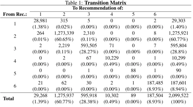
Table 1:Transition Matrix
To Recommendation of:
From Rec.: 1 2 3 4 5 6
1 28,981 (1.38%) 315 (0.02%) 5 (0.00%) 0 (0.00%) 0 (0.00%) 2 (0.00%) 29,303 (1.40%) 2 264 (0.01%) 1,273,339 (60.65%) 2,310 (0.11%) 0 (0.00%) 0 (0.00%) 8 (0.00%) 1,275,921 (60.77%) 3 2 (0.00%) 2,219 (0.11%) 593,505 (28.27%) 71 (0.00%) 0 (0.00% 7 (0.00%) 595,804 (28.8%) 4 0 (0.00%) 2 (0.00%) 67 (0.00%) 10,229 (0.49%) 0 (0.00%) 1 (0.00%) 10,299 (0.49%) 5 0 (0.00%) 0 (0.00%) 1 (0.00%) 0 (0.00%) 88 (0.00%) 1 (0.00%) 90 (0.00%) 6 21 (0.00%) 62 (0.00%) 30 (0.00%) 2 (0.00%) 1 (0.00%) 187,485 (8.93%) 187,601 (8.94%) Total 29,268 (1.39%) 1,275,937 (60.77%) 595,918 (28.38%) 10,302 (0.49%) 89 (0.00%) 187,504 (8.93%) 2,099,522 (100%)
Table 93contains descriptive statistics for the recommendation data-set, indicating: the av-erage number of analysts per each covered firm, the total number of analysts and of brokers. 2I/B/E/S provides a recommendations stop file which includes those analysts estimates that are not
updated or confirmed for a total of six months. According to the description provided by I/B/E/S, recom-mendations are updated by a contributing analyst sending a confirmation, revision or drop in coverage
Finally, also the average rating, among all covered firms, is reported. In this regard, it is in-teresting to note that this number is almost constant over the whole time-frame. To determine whether analysts’ recommendations are predictive of future returns, several portfolios, based on the consensus rating of each covered firm, will be constructed.
Table 2 contains a 6 x 6 transition matrix of the analysts’ average recommendations. In particular, the average analyst rating, ˆCi,t, for the firmion the datet is found by summing the individual ratingsCi,j,t, of the j=1 toni,t analyst who have outstanding recommendations for the firmion dayt and dividing byni,t. More formally:
ˆ
Ci,t= 1
ni,t ni,t
∑
j=1
Ci,j,t (1)
the existence of transaction costs accounts in investors’ decision to re-balance their portfolio or not.
4
Methodology
4.1
Portfolio Construction
In order to build the portfolios that were be used for the analysis, equation 1 was used as a starting point. Hence, five portfolios were constructed: the first one containing stocks whose average rating is 1Cˆi,t 1.5, the second one is defined by 1.5<Cˆi,t 2, the third one is 2<Cˆi,t 2.5, the fourth one is 2.5<Cˆi,t3 and the fifth one consists of the least favorably recommended stocks, for which ˆCi,t>3.
Even though the number of portfolio and the rating cutoffs for each of them are chosen arbi-trarily, they are certainly reasonable. Five portfolios were chosen to achieve an higher degree of separation across the firms which compose the sample while retaining sufficient information for the tests that will be performed. The cutoffs were set so that only the bottom portfolio contains firms whose consensus rating corresponded to hold or sell recommendations. This is due to the relative infrequency of such average ratings among the stocks that compose the S&P 500.
After determining the composition of each portfolio, as of the closing of trading on datet, both the value-weighted and the equal-weighted return for datet+1 were calculated. Denoted byRP,t+1, the return for the value-weighted portfolioPis given by:
RP,t+1= nP,t
∑
i=1
xi,tRi,t+1, (2)
xi,t Represents the market value of equity for firm i as of the close of the trading on datet divided by the aggregate market capitalization of all firms in portfolioPas of the close of trading on that date;
Ri,t+1 Is the log-return4on the stock5of the firmiduring datet+1;
nP,t Represents the number of firms in portfolioPat the close of trading on datet.
For the equal-weighted portfolio, the return, denoted by ¯RP,t, is given by:
¯
RP,t= 1
nP,t nP,t
∑
i=1
Ri,t+1. (3)
The decision of using a value-weighted allocation, beside an equally-weighted one, was moved by two reasons. First, an equal weighting of daily returns (and the implicit assumption of daily rebalancing) leads to portfolio returns that are overstated6. Second, while an individual investor could hold equal amounts of each security, in aggregate each firm must be held in proportion to its market value.
The cumulative return for each portfolio Pis given by the sum of the daily return RP,t over the
ntrading days that constitute the sample:
RP,n= n
∑
t=1
RP,t. (4)
4.2
Performance Evaluation
Three measures of abnormal performance were calculated for each of the constructed portfolios. First, the Capital Asset Pricing Model was employed, estimating the following time-series OLS
4The log-returnR
i,t+1is defined as ln(PiP,ti+,t1). 5In this study only common stocks are considered.
6In this regard, the same approach used by Barber et al. (2001) was followed. The authors argue that the
regression:
RP,t Rf,t=αP+βP(Rm,t Rf,t) +εP,t (5)
where:
Rf,t Is the daily return on treasury bills having one month until maturity7;
αP Represent the estimated CAPM intercept;
βP Is the estimated market beta;
Rm,t Is the daily return on the market index. In this study, daily data for theCRSPIndex were used.
εP,t Is the regression’s stochastic term.
Second, the three-factor model developed by Fama and French (1993) was used. To asses the performances of each portfolio, the following regression was estimated:
RP,t Rf,t =αP+β1,P(Rm,t Rf,t) +β2,PSMBt+β3,PHMLt+εP,t (6)
where:
SMBt Is the difference between the daily returns of a value-weighted portfolio of small stocks and one of large stocks;
HMLt Is the difference between the daily returns of a value-weighted portfolio of high book-to-market stocks and one of low book-to-book-to-market stocks8;
7This return is derived from Ibbotson Associates.
8A more detailed description of both factors is contained in Fama and French (1993). The data used for this
Finally, a third regression was also estimated using the data for price momentum as in Carhart (1997). The resulting regression is:
RP,t Rf,t =αP+β1,P(Rm,t Rf,t) +β2,PSMBt+β3,PHMLt+β4,PU MDt+εP,t (7)
whereU MDt is the equally-weighted monthly average return of the firms with the highest 30 percent return over the the eleven previous months, less the equally-weighted monthly average return of the firms with the lowest 30 percent return over the same period.
In the following analysis, the estimatedβ1,P,β2,P,β3,P andβ4,P are used to provide insights into the characteristics of the firm in each of the portfolios. In particular, a value ofβ1,P greater (less) than one indicates that the firms in the portfolioPare, on average, riskier (less risky) than the market. A value ofβ2,P greater (less) than zero implied that a portfolio tilt toward smaller (larger) firms. A value ofβ3,P greater (less) than zero signifies a tilt toward stocks with a high (low) book-to-market ratio. A value ofβ4,P bigger than zero identifies a portfolio with stocks that have, on average, performed well (poorly) in the past.
Lastly, a more technical premise has to be specified. All the previous model can be ex-pressed, using the matrix notation, as9:
y=Xβ+ε
WhereE[ε] =0andE[εε0] =Φ, which is a positive definite matrix. Under these specification, the OLS estimator ˆβ= (XX0) 1X0yis best linear unbiased with:
Var βˆ = X0X 1X0ΦX X0X 1 (8)
Furthermore, assuming that the errors are homoscedastic, i.e. they have the same variance, it impliesΦ=σ2I. Hence, equation 8 simplifies to:
Var βˆ =σ2 X0X 1
Defining the residuals asei=yi xiβ, whereˆ xiis theith row ofX, the OLS covariance matrix
is:
Σ= ∑
N i=1e2i
N K (X
0X) 1 (9)
where N is the sample size and K is the number of regressors. However, Σis appropriate for hypothesis testing and computing confidence intervals only when the standard assumptions of the regression model, including homoscedasticity hold. Furthermore, if equation 9 is used in presence of heteroscedasticity, results are likely to be misleading. Since in practice the form of heteroscedasticity is unknown, a heteroscedasticity robust covariance matrix(Σˆ)should be used (Long and Ervin, 2000). The basic idea, as shown by White (1980), is then to use e2i
to estimate φii. This can be seen as estimating the variance of εi with a single observation: ˆ
φii= (ei 0)2/1=e2i. Than, an estimator for Φof equation 8 isΦˆ =diag
⇥
e2i⇤. Therefore, a first heteroscedasticity robust estimator is:
HC0= X0X 1X0ΦˆX X0X 1= X0X 1X0diag⇥e2i⇤X X0X 1 (10)
As shown by White (1980), the estimator in equation 10 is a consistent for Var βˆ in the presence of heteroskedasticity of an unknown form.
factor ofpN/(N K). Whit this correction, the resulting estimator is HC1:
HC1= N
N K X
0X 1
X0diag⇥e2i⇤X X0X 1= N
N KHC0
The idea behind this new estimator is that Φˆ of equation 10 is based on the residuals of the regression, e, and not on the true errors ε. Hence, even if the errors are homoscedastic, the residual might not be. Furthermore, defininghii=xi(X0X) 1x0i, then:
Var(ei) =σ2(1 hii)6=σ2 (11)
Since 1/Nhii1,Var(ei)underestimatesσ2. Equation 11 indicates that whilee2i is a biased estimator ofσi2,e2i/(1 hii)will be less biased10. Basing themselves on the work by Horn et al. (1975), MacKinnon and White (1985) proposed a new estimator:
HC2= X0X 1X0diag
e2i
1 hii
X X0X 1
Finally, a third variation approximates a more complicated “jackknife” estimator, first devel-oped by Efron and Morris (1972):
HC3= X0X 1X0diag
e2i
(1 hii)2
X X0X 1 (12)
Dividing e2i by(1 hii)2 inflatese2i which is thought to adjust for the “over-influence” of ob-servations with large variances (Long and Ervin (2000)). For the sake of this study, all the presented standard errors were estimated using equation 12.
5
Portfolio Characteristics and Returns
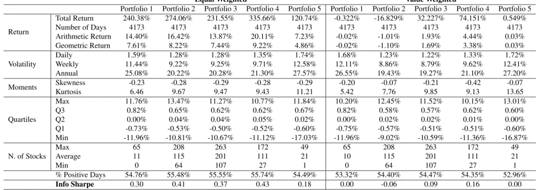
Table 2 provides descriptive statistics on the performances of the portfolios built according to analyst recommendations, whose cumulative returns are drown in Figures 1 and 2.
Looking at the first half of the table, it can be observed that, among the equally weighted portfolios, the one containing stocks whose average rating was between 2.5 and 3 performed the best, both in terms of average return and of Info Sharpe ratio. It is worth noting that, beside Portfolio 5, which contains the least recommended stocks, all of the other portfolios outperformed the one containing the most recommended companies.
Figure 1: Equally Weighted Portfolio Cumulative Return.
assets in the portfolio.
Table 2:Portfolio Performance Statistics
Equal Weighted Value Weighted
Portfolio 1 Portfolio 2 Portfolio 3 Portfolio 4 Portfolio 5 Portfolio 1 Portfolio 2 Portfolio 3 Portfolio 4 Portfolio 5
Return
Total Return 240.38% 274.06% 231.55% 335.66% 120.74% -0.322% -16.829% 32.227% 74.151% 0.549%
Number of Days 4173 4173 4173 4173 4173 4173 4173 4173 4173 4173
Arithmetic Return 14.40% 16.42% 13.87% 20.11% 7.23% -0.02% -1.01% 1.93% 4.44% 0.03%
Geometric Return 7.61% 8.22% 7.44% 9.22% 4.86% -0.02% -1.10% 1.69% 3.38% 0.03%
Volatility
Daily 1.59% 1.28% 1.28% 1.35% 1.74% 1.68% 1.23% 1.22% 1.33% 1.72%
Weekly 11.44% 9.22% 9.25% 9.71% 12.58% 12.11% 8.86% 8.79% 9.62% 12.41%
Annual 25.08% 20.22% 20.28% 21.30% 27.57% 26.55% 19.43% 19.27% 21.10% 27.20%
Moments Skewness -0.23 -0.28 -0.29 -0.28 -0.29 -0.20 -0.07 -0.21 -0.42 -0.07
Kurtosis 6.46 9.67 9.47 9.43 11.21 5.42 7.76 9.85 9.13 13.65
Quartiles
Max 11.76% 13.47% 11.27% 10.77% 11.84% 10.20% 12.45% 11.52% 10.15% 13.01%
Q3 0.82% 0.65% 0.62% 0.62% 0.67% 0.82% 0.58% 0.57% 0.62% 0.60%
Q2 0.00% 0.04% 0.04% 0.05% 0.02% 0.00% 0.02% 0.02% 0.01% 0.00%
Q1 -0.73% -0.53% -0.50% -0.52% -0.60% -0.75% -0.57% -0.51% -0.51% -0.60%
Min -11.96% -10.81% -10.67% -11.12% -17.03% -11.96% -9.02% -10.59% -11.36% -16.87%
N. of Stocks
Max 65 208 263 172 49 65 208 263 172 49
Average 11 115 201 111 21 10 115 201 111 21
Min 0 64 107 27 1 0 64 107 27 1
% Positive Days 54.76% 55.48% 55.55% 55.74% 54.49% 53.32% 54.40% 54.47% 54.35% 52.96%
Info Sharpe 0.30 0.41 0.37 0.43 0.18 0.00 -0.06 0.09 0.16 0.00
Table 3: Portfolios Market Capitalization
Portfolio 1 2 3 4 5
Market Capitalization
Max 19.09% 68.92% 59.24% 34.72% 6.24%
Average 2.39% 34.00% 45.49% 15.44% 2.01%
Min 0.00% 18.77% 14.04% 1.33% 0.00%
Table 4: Average Annual Turnover
Equally Weighted Portfolios Value Weighted Portfolios
Portfolio 1 2 3 4 5 1 2 3 4 5
Portfolio Turnover 781.93% 347.96% 313.94% 373.04% 462.64% 895.61% 482.85% 479.88% 630.06% 695.95%
Figure 2: Value Weighted Portfolio Cumulative Return.
As far as the value weighted portfolios, it appears that the previous results hold as well. Moreover, the patterns in the market risk factor and HML are clearer. The same can be said regarding the momentum factor. Looking at theAd justedR2, they indicates that the results of the regression are solid.
Table 5:Equal Weighted Portfolios: Regressions Results Equal Weighted Portfolios
CAPM Three Factor Model Four Factor Model
Portfolio Intercept βP R-SquaredAdjusted Intercept Mkt-Rf SMB HML R-SuaredAdjusted Intercept Mkt-Rf SMB HML UMD R-SquaredAdjusted
1 0.00 (0.24) 0.09 (7.05) 0.01 0.00 (0.41) 0.16 (4.89) 0.99 (55.54) 0.22 (7.13) 0.34 0.00 (0.43) 0.15 (4.88) 0.98 (55.88) 0.22 (7.25) -0.015 (-0.78) 0.54
2 (1.54)0.00 (0.63)0.04 0.01 (2.37)0.001 (5.63)0.08 (105.11)0.98 (4.53)0.07 0.45 0.0001(2.07) (16.96)0.11 (106.28)0.998 (3.74)0.06 (6.68)0.05 0.70
3 0.01 (1.19) 0.28 (4.56) 0.02 0.00 (1.07) 0.31 (17.63) 0.98 (125.25) 0.01 (0.74) 0.31 0.00 (1.29) 0.30 (16.98) 0.96 (115.97) 0.02 (1.98) -0.04 (-3.94) 0.70 4 0.00 (1.29) 0.49 (7.08) 0.05 0.00 (1.11) 0.54 (30.37) 0.99 (106.33) 0.10 (4.77) 0.29 0.00 (1.75) 0.49 (30.13) 0.95 (106.28) 0.125 (6.67) -0.125 (-13.10) 0.68 5 0.00 (0.81) 0.70 (7.05) 0.07 -0.01 (-1.03) 0.76 (16.19) 1.06 (49.21) 0.18 (3.44) 0.29 -0.001 (-0.62) 0.66 (15.87) 0.99 (41.52) 0.22 (4.52) -0.25 (-9.31) 0.56
Table 6: Value Weighted Portfolios: Regressions Results
Value Weighted Portfolios
CAPM Three Factor Model Four Factor Model
Portfolio Intercept βP R-SquaredAdjusted Intercept Mkt-Rf SMB HML R-SuaredAdjusted Intercept Mkt-Rf SMB HML UMD R-SquaredAdjusted
1 0.00 (0.71) -0.10 (-1.21) 0.01 0.00 (-1.22) -0.057 (-1.56) 1.06 (52.23) 0.08 (2.39) 0.30 0.00 (-1.27) -0,05 (-1.28) 1.07 (51.57) 0.07 (2.23) -0.03 (1.10) 0.54 2 0.00 (-0.06) -0.18 (-2.92) 0.01 -0.001 (-3.69) -0.17 (-14.70) 0.96 (157.83) -0.17 (-17.15) 0.33 -0.0001 (-4.30) -0.15 (-13.69) 0.98 (169.28) -0.19 (-18.11) 0.08 (12.30) 0.75
3 (0.15)0.0 (3.57)0.20 0.02 (-2.10)-0.001 (9.81)0.197 (115.09)0.93 (-11.3)-0.20 0.31 (-2.00)0.00 (9.44)0.19 (105.97)0.93 (-11.53)-0.20 (-1.23)-0.01 0.72
6
Further Analysis
In this section, the effect of changing how the portfolio are constructed is evaluated. Further-more, the analysts’ recommendation sample will be also split. First, by subperiod, and then by market direction.
6.1
Changing Portfolio Attributions
Previously, the portfolios’ components were decided according to their raw average recommen-dation. In this section, each score was standardized. To do so, the row average (corresponding to the average recommendation for each day in the sample) was subtracted from each element of the score matrix (S) which were than divided by the standard deviation of each row. Mathe-matically, given the matrixS, of sizem⇥n:
Sm,n=
0 B B B B B B B B B B @
s1,1 s1,2 · · · s1,n
s2,1 s2,2 · · · s2,n
..
. ... . .. ...
sm,1 sm,2 · · · sm,n
1 C C C C C C C C C C A
Ifµnandσnare, respectively, the mean and the standard deviation of the observations contained in the in the columnn, the standardized matrix ( ¯S) is given by:
¯
Sm,n=
0 B B B B B B B B B B @
s1,1 µ1
σ1
s1,2 µ2
σ2 · · ·
s1,n µn
σm
s2,1 µ1
σ1
s2,2 µ2
σ2 · · ·
s2,n µn
σm
..
. ... . .. ... sm,1 µ1
σ1
sm,2 µ2
σ2 · · ·
sm,n µn
σm 1 C C C C C C C C C C A
equal to the first quintile of the specific row; portfolio two was composed of stocks whose rating was between the first quintile and the second one and so on. The performance achieved by this new portfolios are presented in table 1011. As the table shows, there is no significant difference in terms of performances in the case of the equal weighted portfolios. However, looking at the data for the value weighted ones, an increase in the Sharpe Ratios, which are now positive, can be noticed. The results of Carhart’s Four Factor Model are presented in table 11.12 Again, the results are similar to the one obtained previously, with, in the case of the equal weighted portfolios, all the coefficients statistically different from zero and a null intercept. In the case of value weighted portfolios, intercepts are negative for portfolio two and three. Moreover, w the other coefficients are almost always different from zero. Looking for the patterns that were previously identified, it can be noticed that:
• What was said for the market risk premium still hold: riskier stocks receive lower ratings;
• Lower ratings seems to be associated with stocks characterized by lower book-to-market
ratios;
• The analyst are trend following: higher coefficients for the momentum factor are
associ-ated with top-rassoci-ated stocks.
6.2
Subperiod Analysis
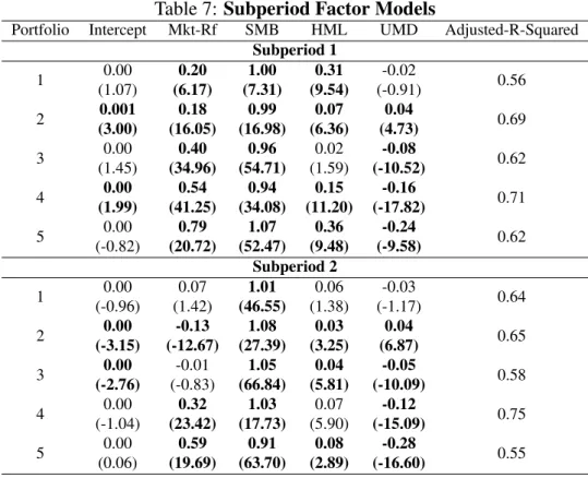
Following the approach of Barber et al. (2001), a subperiod analysis for the factor models was carried out13. To do so, the sample was split in two halves, the first one covering a period from January 2000 to December 2008 and the second one from January 2009 to December 2015.
11This table is presented in the enclosed appendix. 12This table is presented in the enclosed appendix.
13In this paragraph, only equally weighted portfolios are presented since the results obtained from the value
Table 7: Subperiod Factor Models
Portfolio Intercept Mkt-Rf SMB HML UMD Adjusted-R-Squared
Subperiod 1 1 0.00 (1.07) 0.20 (6.17) 1.00 (7.31) 0.31 (9.54) -0.02 (-0.91) 0.56
2 (3.00)0.001 (16.05)0.18 (16.98)0.99 (6.36)0.07 (4.73)0.04 0.69
3 0.00 (1.45) 0.40 (34.96) 0.96 (54.71) 0.02 (1.59) -0.08 (-10.52) 0.62 4 0.00 (1.99) 0.54 (41.25) 0.94 (34.08) 0.15 (11.20) -0.16 (-17.82) 0.71 5 0.00 (-0.82) 0.79 (20.72) 1.07 (52.47) 0.36 (9.48) -0.24 (-9.58) 0.62 Subperiod 2 1 0.00 (-0.96) 0.07 (1.42) 1.01 (46.55) 0.06 (1.38) -0.03 (-1.17) 0.64 2 0.00 (-3.15) -0.13 (-12.67) 1.08 (27.39) 0.03 (3.25) 0.04 (6.87) 0.65 3 0.00 (-2.76) -0.01 (-0.83) 1.05 (66.84) 0.04 (5.81) -0.05 (-10.09) 0.58 4 0.00 (-1.04) 0.32 (23.42) 1.03 (17.73) 0.07 (5.90) -0.12 (-15.09) 0.75 5 0.00 (0.06) 0.59 (19.69) 0.91 (63.70) 0.08 (2.89) -0.28 (-16.60) 0.55
The results from the factor model regressions are presented, for both subperiods, in table 7. Coefficients for Subperiod 1 show that for both portfolio two and four a significant, yet very small, alpha was generated. Furthermore, both the trends for the firm size and for the momentum still appear. However, it should be noticed that the Ad justedR2 are now smaller than the previous ones.
Looking at Subperiod 2, it appears that all the significant alphas are now negative and, again, very small. It seems that the market risk premium trend do not apply for this subset. However, the momentum trend still holds. Furthermore, it seems that the pattern for the firms’ book-to-market ratio is present in this subset. As far as the measure of fit, they are very similar to the one obtained in the first subset and smaller than the original ones.
alphas were negative. The only trend that seems to persist among both subsets is the one for momentum. This means that analysts are always inclined to recommend stocks that performed better in the past and, hence, they can be considered as trend-following.
6.3
Bull Market Vs. Bear Market
In this section, the performances of analysts’ recommendations were tested in condition of bull and bear market. To define bull and bear market, the same approached followed by Barber et al. (2001) is used: a month is considered of bull market if the return on theCRSPIndex was positive, bear otherwise. Then, observation for portfolio returns were split accordingly. Hence two samples were created, one with 2325 observations, corresponding to a bull market, and one with 1846 observations, corresponding to a bear market. The results from the Carhart’s Four Factor model are presented in tables 12 and 13.14
As far as the bull market sample, it appears that, portfolio two, three and four were capable of generating small positive alphas. However, just as it happened before, it is not portfolio one to achieve the bigger alpha, which, in this case, is not statistically different from zero. Moreover, the only visible pattern seems to be the one for the momentum factor. The same results apply also in the case of the value weighted portfolios. However, it should be noticed that in this case the top-rated portfolios are associated to negative betas for the market risk factor. Hence, this might represent one of the possible explanations for the small performance of the portfolios: when the market is bullish, they do not catch all the movement.
In the case of the bear market sample, we can notice that, for the equal weighted Portfolios, number one and two were capable of generating a small positive alpha. However, Portfolio five did so as well. Furthermore, it appears that the pattern for the market risk premium is present: during bearish months, analysts attributed less favorable recommendation to stocks that have an
higher beta towards the market. Moreover, also the patter for momentum is still present, again. In the case of the value weighted portfolios, only Portfolio 1 generated a positive alpha, whereas Portfolio two generated a negative one. Furthermore, the pattern for the market risk premium is present and it is even stronger than in the previous case. The same can be said for the pattern associated with the momentum factor.
7
Trading Strategy
As already mentioned, Elton et al. (1986) have indicated that there is information laying into analysts’ change in recommendations. Hence, a trading strategy that is based on the on the change in the average score should yield a positive return. To test this hypothesis, a series of long-short portfolios were constructed using the previous sample.
In order to build these portfolio, the starting point was the score matrix S, of dimension
m⇥n:
Sm,n=
0
B B B B B B B B B B B B B B @
s1,1 s1,2 · · · s1,j · · · s1,n
..
. ... · · · ... · · · ...
si,1 si,2 · · · si,j · · · si,n
..
. ... · · · ... . .. ...
sm,1 sm,2 · · · sm,j · · · sm,n
1
C C C C C C C C C C C C C C A
Tm,n= 0 B B B B B B B B B B B B B B B B B B B B B B @
t1,1 t1,2 · · · t1,j · · · t1,n
..
. ... · · · ... · · · ...
ti+d,1 ti+d,2 · · · ti+d,j · · · ti+d,n
..
. ... · · · ... · · · ...
ti+d+hp,1 ti+d+hp,2 · · · ti+d+hp,j · · · ti+d+hp,n
..
. ... · · · ... . .. ...
tm,1 tm,2 · · · tm,j · · · tm,n
1 C C C C C C C C C C C C C C C C C C C C C C A
The main idea behind the trading strategy is to go long (short) in that stocks that have received an upgrade (downgrade) in the average score. In this regard, the position is held for different periods: from three days to three months. The results of this strategy are presented in table 8.
Table 8:Long-Short Equity Portfolios with Different Holding Periods
Holding Period 3 Days 15 Days 30 Days 45 Days 60 Days 90 Days
Return
Total Return -15.69% 516.73% 732.19% 752.76% 753.21% 818.25%
Number of Days 4173 4173 4173 4173 4173 4173
Arithmetic Returns -1.00% 32.81% 46.50% 47.80% 47.83% 51.96%
Geometric Returns -1.08% 12.25% 14.40% 14.58% 14.58% 15.12%
Volatility
Daily 1.11% 2.20% 2.62% 2.61% 2.60% 2.60%
Weekly 7.99% 15.85% 18.91% 18.82% 18.78% 18.74%
Annual 17.53% 34.76% 41.45% 41.27% 41.19% 41.10%
Moments Skewness 0.88 -0.23 -0.35 -0.34 -0.33 -0.34
Kurtosis 62.16 12.42 9.24 9.4 9.62 9.71
Quartiles
Max 16.93% 20.21% 21.20% 21.70% 21.70% 21.93%
Q3 0.00% 0.71% 1.21% 1.21% 1.21% 1.20%
Q2 0.00% 0.00% 0.03% 0.02% 0.02% 0.02%
Q1 0.00% -0.46% -0.98% -0.96% -0.96% -0.95%
Min -14.98% -21.28% -21.28% -21.11% -21.38% -21.43%
% Positive Days 9.03% 37.24% 50.59% 50.42% 50.44% 50.71%
Turnover 2300.50% 2288.52% 1249.36% 798.21% 782.53% 357.57%
Info Sharpe -0.06 0.94 1.12 1.16 1.16 1.26
extend-Figure 3: Long-Short Trading Strategy with Different Holding Periods.
ing the holding produce higher Sharpe Ratios. However, these increases are not of the same magnitude as the first one.
References
Brad Barber, Reuven Lehavy, Maureen McNichols, and Brett Trueman. Can investors profit from the
prophets? security analyst recommendations and stock returns. The Journal of Finance, 56(2):531–
563, 2001.
Brad M Barber and Terrance Odean. Boys will be boys: Gender, overconfidence, and common stock
investment. Quarterly journal of Economics, pages 261–292, 2001.
David A Belsey, Edwin Kuh, and Roy E Welsch. Regression diagnostics: Identifying influential data
and sources of collinearity. John Wiley, 1980.
Mark M Carhart. On persistence in mutual fund performance. The Journal of finance, 52(1):57–82,
1997.
Hemang Desai, Bing Liang, and Ajai K Singh. Do all-stars shine? evaluation of analyst
recommenda-tions. Financial Analysts Journal, 56(3):20–29, 2000.
Bradley Efron and Carl Morris. Limiting the risk of bayes and empirical bayes estimatorspart ii: The
empirical bayes case. Journal of the American Statistical Association, 67(337):130–139, 1972.
Edwin J Elton, Martin J Gruber, and Seth Grossman. Discrete expectational data and portfolio
perfor-mance. The Journal of Finance, 41(3):699–713, 1986.
Eugene F Fama and Kenneth R French. Common risk factors in the returns on stocks and bonds.Journal
of financial economics, 33(1):3–56, 1993.
Sanford J Grossman and Joseph E Stiglitz. On the impossibility of informationally efficient markets.The
American economic review, 70(3):393–408, 1980.
David V Hinkley. Jackknifing in unbalanced situations. Technometrics, 19(3):285–292, 1977.
Susan D Horn, Roger A Horn, and David B Duncan. Estimating heteroscedastic variances in linear
Narasimhan Jegadeesh and Woojin Kim. Do analysts herd? an analysis of recommendations and market
reactions. Review of Financial Studies, 23(2):901–937, 2010.
J Scott Long and Laurie H Ervin. Using heteroscedasticity consistent standard errors in the linear
regres-sion model. The American Statistician, 54(3):217–224, 2000.
James G MacKinnon and Halbert White. Some heteroskedasticity-consistent covariance matrix
estima-tors with improved finite sample properties. Journal of econometrics, 29(3):305–325, 1985.
Burton G Malkiel and Eugene F Fama. Efficient capital markets: A review of theory and empirical work.
The journal of Finance, 25(2):383–417, 1970.
I Welch. Herding among security analysts’, journal of financial economics, 58, 369-96.
INTERNA-TIONAL LIBRARY OF CRITICAL WRITINGS IN ECONOMICS, 187(2):606, 2005.
Halbert White. A heteroskedasticity-consistent covariance matrix estimator and a direct test for
het-eroskedasticity. Econometrica: Journal of the Econometric Society, pages 817–838, 1980.
Kent L Womack. Do brokerage analysts’ recommendations have investment value? The journal of
finance, 51(1):137–167, 1996.