Exploring the effects of visual occlusion in young football players during small-sided games

(1)

University of Trás-os-Montes and Alto Douro

Exploring the effects of visual occlusion in young football

players during small-sided games

Master Thesis in Performance Analysis in Sports

Gabriel Joaquim Gonçalves Vilas Boas

Supervisor: Professor Doctor Jaime Sampaio

(2)

(3)

University of Trás-os-Montes and Alto Douro

Exploring the effects of visual occlusion in young football

players during small-sided games

Master Thesis in Performance Analysis in Sports

Gabriel Joaquim Gonçalves Vilas Boas

Supervisor: Professor Doctor António Jaime da Eira Sampaio

Judge composition:

Professor Doctor Nuno Miguel Correia Leite Professor Doctor António Jaime da Eira Sampaio Professor Doctor Bruno Sérgio Varanda Gonçalves

(4)

The following knowledge and ideas shown in this thesis, are exclusively responsible by the author.

(5)

Acknowledgements

I would like to express my sincere gratitude to the University of Trás-os-Montes and Alto Douro, for accepting me as a student and enrol me in the International Masters of Performance Analysis in Sports.

I would also like to thank to the professor Diogo Coutinho for the help and letting me perform this study in his football team. As well for the players that participated in this study. Thanks to professor Nuno Leite for always be helpful with any kind of questions and problems that I had, and to give me advice in my academic journey.

A special thanks to the professor Bruno Gonçalves, that always helped me in order to achieve the correct data collection and the analysis of the results of this study. To my advisor Jaime Sampaio, for his understanding, wisdom, insight and feedback that he gave me in this study. And for always bringing the best insight and knowledge surrounding this study.

And finally, I would like to thank my parents and sister, for always giving me support in this journey of knowledge, in order to achieve my academic responsibilities and above all, my dreams.

(6)

Abstract

The aim of this study was to identify the physical, tactical and technical performances of young footballers, when playing without and with a visual occlusion. The tasks were five-minutes matches (5 versus 5 players) in two different pitch dimensions (small pitch – 40m x 30m and big pitch – 50m x 35m). The visual occlusion was a constraint applied to the players, where they wore a band occluding the sight of one eye. The occluded eye was on the same side as their dominant foot.

This study is in line with a nonlinear pedagogy approach, which accentuates the need to design representative and facilitative type of learning for individual learners, supported by principles in understanding the nonlinearity features of human learning. In order to extract, analyse and interpret the results for this study, the physical, tactical and technical data was obtained. For the physical and tactical variables, the coordinates of the players were needed. As for the technical variables, the video recordings were required. The magnitude-based inferences and precision of estimation was employed aiming to avoid the shortcomings of research approaches supported by the null-hypothesis significance testing.

The results show that walking intensity, presents a possibly and most likely increase for both small pitch and big pitch respectably, when players played with bands as oppose without bands. In the total distance covered showed a likely decrease in both small and big pitch while wearing bands as oppose without bands. In the tactical variables, regarding the distance to own team centroid, showed a possibly decrease for without vs with bands and a likely increase for without against with bands vs with against without bands in the small pitch. As for the distance to opponents’ centroid showed a possibly increase in the small pitch for without vs with bands, and a likely increase in the big pitch for with against without bands. The technical variables regarding the number of touches that a player took and the dominant touches showed, a possibly increase for without vs with bands in the small and big pitch scenarios. As for the non-dominant touches, showed possibly increase for both without vs with bands and without against with bands vs with against without bands in the small pitch. In the bid field occurred a likely increase in non-dominant touches for without vs with bands. Results suggest that constraining situations with visual occlusion can created a "team-emergency” situation where players decrease their inter-personal distances and

(7)

consequently slowed game pace and decrease distance covered. Also as a consequence, the number of passes has decreased. This resulted in a more individualistic style of play, recurring to hold possession influencing positively the number of touches that each player took in order to take control the ball. These results were more noticeable when both teams were wearing the bands. The use of the non-dominant foot was greater when the players wore the bands, increasing the use of the non-dominant foot also influenced the passing accuracy of the players.

(8)

Index

Acknowledgements ... iii

Abstract ... iv

Index ... vi

Table Index ... viii

Figures Index ... ix

Abbreviation List ... x

1. Introduction ... 1

1.1 Learning process of task constraints ... 2

1.2 The effects of pitch size manipulations... 3

1.3 Non-linear pedagogy and differential learning ... 5

1.4 Vision ... 6

1.4.1 Sports vision... 6

1.5 Foot-eye coordination ... 7

1.6 Perceiving affordances for others ... 7

1.7 Temporal occlusion ... 8

1.8 Visual search behaviour ... 8

1.9 Advance visual cue utilization ... 9

1.10 Knowledge of situational probabilities ... 9

1.11 Objective ... 10

2. Methods ... 11

2.1 Experimental Approach to the Problem ... 11

2.2 Participants ... 11 2.3 Experimental task ... 12 2.4 Procedures ... 13 2.5 Pitch-positioning derived-variables ... 15 2.6 Statistical analysis ... 16 3. Results ... 17 3.1 Physical Performance ... 17 3.2 Tactical Performance ... 21 3.3 Technical Performance ... 24 4. Discussion ... 30

(9)

5. Conclusions ... 34 6. References ... 35 7. Attachment ... 41

(10)

Table Index

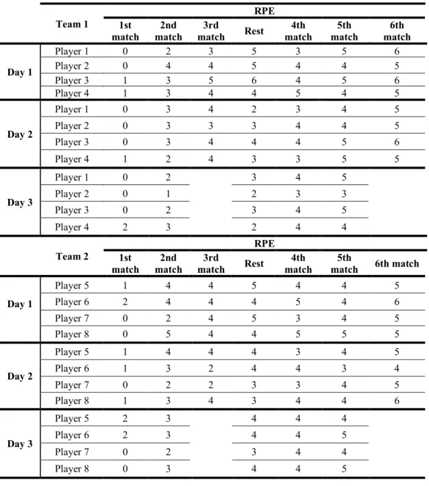
Table 1. Experimental conditions in the small and big pitch ... 11 Table 2. Study protocol ... 13 Table 3. Descriptive physical analysis (mean ± SD). Difference in means and uncertainty in the true differences comparisons among the different constraints among both types of field dimensions. ... 18 Table 4. Descriptive tactical analysis (mean ± SD). Difference in means and uncertainty in the true differences comparisons among the different constraints among both types of field dimensions. ... 21 Table 5. Descriptive technical analysis (mean ± SD). Difference in means and uncertainty in the true differences comparisons among the different constraints among both types of field dimensions. ... 25 Table 6. RPE scale of the study protocol ... 41

(11)

Figures Index

Figure 1. Standardized (Cohen) differences in physical variables according to the two field dimensions (small pitch and big pitch). Error bars indicate uncertainty in the true mean changes with 90% confidence intervals... 20 Figure 2. Standardized (Cohen) differences in tactical variables according to the two field dimensions (small pitch and big pitch). Error bars indicate uncertainty in the true mean changes with 90% confidence intervals... 23 Figure 3. Standardized (Cohen) differences in technical variables according to the two field dimensions (small pitch and big pitch). Error bars indicate uncertainty in the true mean changes with 90% confidence intervals... 28

(12)

Abbreviation List

ACT – Australian Capital Territory ApEn – Approximate entropy CL – Confidence limits

CV – Coefficient of variation GK – Goalkeeper

GPS – Global Positioning System Hz – Hertz

Km/h – Kilometres per hour m - Meters

min – Minute

m/s – Meters per second r – Tolerance factor

RPE – Rated perceived exertion

SSCG – Small sided and conditioned games UTM - Universal Transverse Mercator

(13)

1. Introduction

In course of the years the studies focused on football have been increasing in quantity and quality. Across the literature several authors suggest that sports’ expertise requires as much skill to pick up valuable information as to perform precise movements. The differences in expert and amateur athletes, demonstrate that the expert players showed better performance when using visual information to anticipate the direction of a moving object than amateur or less experienced athletes. This principle seems simple to assimilate, but their previous experience improves the reaction time and enables them to accurate predict, in this case the direction of a moving object. Ando et al. (2001), reported that expert athletes have shorter reaction times than novices, given more developed central and peripheral vision. Furthermore, experts could garner more contextual knowledge of the task, making the decision-making process quicker and more precise. For that is necessary to understand the nonlinearity nature of human learning. Teaching and coaching this nonlinearity is based on ideas from Newell (1986) and Davids et al. (2008), a constraints-led approach has been strongly presented to promote the understanding of how goal-directed behaviour can emerge as a consequence of the interacting constraints (task, environment, and performer) in a learning or performance situation (Renshaw et al., 2010). Specifically, performer constraints refer to the structural and functional aspects of the learner; environment constraints incorporate the physical and the social-cultural environment; and rules of game; and equipment and goals of the task can be categorized as task constraints (Davids et al., 2008). However, a constraints-led approach only promotes the understanding of how skills is acquired from a motor learning domain and does not provide a framework for designing motor learning programs.

An important aspect of nonlinear pedagogy is associated with the role of functional movement variability in enhancing acquisition of coordination since movement variability is seen as a feature of nonlinearity in human learning (Chow & Atencio, 2012; Chow et al., 2011). Nonlinear pedagogy incorporates and recognizes the critical role of infusing perturbation (e.g., in the form of encouraging variability in practice conditions) in a learning environment to allow for exploratory learning and greater search in the perceptual-motor workspace of the individual. This is especially relevant when a learner is stuck in a rut and the coach can incorporate a perturbation to the

(14)

practice by altering task constraints, such as instructions or equipment to challenge the learner to try new coordination patterns.

In this study, the players tested were young amateur players, with enough basic skillset to play football. Also, to take into account is the different levels of relationship express the dynamics of interpersonal coordination established between players, both within teammates and between opponents, bounded by ongoing changes in the performance environment (Duarte et al., 2012). This is very important, due to the fact that, during a football match the players are directly influenced by all of the surrounding factors such as pitch size, teammates, opponents and so on. To give a more precise and scientific evaluating of these factors, several positioning derived-variables such as centroid estimation, distance covered and game pace, have been used to disclose the effect of relevant constraints on collective behaviours. The study of the manipulation of spatial referents, such as pitch task dimensions (Silva et al., 2014). These experiments generally show that inter-team adaptations on the spatiotemporal relationships between players and on preferential pitch exploration, tend to occur as a result of changing these spatial referents. At the same time, the physical demands of several task constraints have been well described in literature (Hill-Haas et al., 2011).

1.1 Learning process of task constraints

The learning process of a new constraint is a new reality, that players on the initial phases of the learning process tend to freeze their degrees of freedom in order to take advantage of a stable context to achieve a task goal (Edwards, 2010), but as the learning process proceeds, the exploration of different behaviours allows for greater movement possibilities. This only takes advantage, if the players feel comfortable with the new constraint, because sometimes to many new inputs could be a problem greater than the player could handle, especially amateur players. With that in mind, coaches should manipulate the tasks constraints in order to change the players’ possibilities of action, and consequently promote higher-level performances. Breaking down the complexity of the constraints to better suit the squad of players that he has. For instance, affecting the space of intervention during the training tasks may amplify the information that should be attended for effective decisions. This topic has not been researched well enough, in order to describe the spatial-temporal relationships on players’ during practice, however, this issue deserves a closer look considering that high-level football

(15)

performances seems to be related to optimized intra-team movement synchronizations (Folgado et al., 2014; Folgado et al., 2015; Frencken et al., 2012). The role of constraints has been put forth as an important aspect of nonlinear pedagogy. While much has been written about the constraints-led approach and its role in skill acquisition (Renshaw et al., 2012), it only provides an understanding of how goal-directed behaviour occurs. Nonlinear pedagogy is reinforced by this understanding of how key constraints interact with each other for coordination to self-organize in a performance or learning setting. Constraints are defined as providing the boundaries where the learners can explore and search for movement solutions afforded to the individual within a perceptual-motor workspace (Chow et al., 2006; Chow et al., 2007).

Typically, task constraints, such as instructions, rules of the activity, and equipment, can be readily manipulated to perturb learners to explore and acquire different movement behaviours (Chow & Atencio, 2012; Tan et al., 2012).

Task constraints such as task goals, specific rules, surfaces, performance areas, player-starting positions, number of players involved, etc., are linked by the goal of the activity and are influenced by the goal (Davids, Button, & Bennett, 2008; Passos et al., 2008). Task-constraints manipulation is the most powerful tool available to coaches for improving the players’ decisions and actions in a performance context (Passos et al., 2008) since their influence can override the effects of other relevant constraints (Davids, Button, & Bennett, 2007). With that, manipulating the pitch size and visual constraints, seems a powerful tool for the players to perform and adapt to a total different set of situations that will put them exposed and forced them to leave their comfort zone.

1.2 The effects of pitch size manipulations

The pitch size was manipulated in this experiment in order to see the different changes in physical, tactical and technical behaviour of the players. According to previous research on SSCGs in football, involving pitch size manipulations, has mainly focused on physical and technical characteristics of performance (Kelly & Drust, 2008; Owen, Twist, & Ford, 2004; Tessitore et al., 2006). Some studies suggest that shorter and narrower pitches resulted in smaller longitudinal and lateral inter-team distance values, respectively, whereas a team’s surface area decreased as a result of smaller total playing areas (Frencken et al., 2013). This could mean that the interpersonal relations between

(16)

players and how they were constrained to adapt their interactive behaviour according to specific pitch size constraints. Another approach to the matter is, to talk about the opposition relationship between players of different teams, meaning that at every instant, some or all players aim to achieve a specific goal. Whilst doing so, players within a team are cooperating to score a goal, or to prevent the opposition from scoring. Thus, all players cooperate and compete simultaneously. So, it’s important for the player to keep exploring and moving on the field to choose tactically relevant positions, relative to the teams positioning on the field, relative to opponents, teammates, ball, and specific task goals. With that in mind, information based on speed and direction of players and ball seem to govern tactical decisions by players. This infers that changes in player positions on the field reflect the interactions between players. Some evidence confirms this has been provided in basketball (Araújo et al., 2004) and rugby (Passos et al., 2011). Such entrainment of team measures like the teams’ centroids (geometrical centres) and surface areas has been established in various studies. Moreover, both inter-team distances, defined as the distance between two longitudinal or lateral components of teams’ centroid positions, seem to be associated with critical and tactically relevant game following a dynamical analysis of an elite football match (Frencken et al., 2012). So, the distance between the teams’ centroids and difference in surface area reflect the interaction process between teams. Still there’s the need to dig deeper into the understanding of the effects of pitch size manipulations, and how this constraint manipulates individual tactical behaviour underlying collective performance in SSCGs. These experiments generally show that inter-team adaptations on the spatiotemporal relationships between players and on preferential pitch exploration, tend to occur as a result of changing the spatial referents. At the same time, the physical and physiological demands of several task constraints have been well described in literature.

From the workload viewpoint, using pitch area-restrictions may be useful to manage the physical and physiological stimulus while highlighting specific positioning role demands and maintaining the tactical focus. These outcomes may help coaches to better plan the short- and mid-term schedules by optimizing training loads during the practice sessions. In fact, appropriate weekly stimuli are well-related to recovery strategies and fatigue prevention (Coutinho et al., 2015).

(17)

1.3 Non-linear pedagogy and differential learning

A nonlinear pedagogy approach, based on nonlinear and complexity phenomenon, has increasingly been supported to provide practitioners with key principles to reinforce teaching. Pertinent information on how to assess performance, how to structure practices, and how best to deliver instructions and provide feedback are particularly relevant (Chow et al., 2013). Nonlinear pedagogy accentuates the need to design representative and facilitative type of learning for individual learners supported by principles in understanding the nonlinearity features of human learning. Nonlinear pedagogy provides a pedagogical framework where learning needs to be situated in real-game contexts (Chow et al., 2006). Port and Van Gelder (1995) have emphasized the importance of understanding the development of cognition from a situated and embodied perspective. Learning takes place when the learner is in the context of the learning environment and the acquisition of knowledge occurs as a consequence of the interactions between the learner and the environment. Fajan, Riley and Turvey (2009) reiterated the significance of providing representative learning situations by highlighting that athletes need to be placed in realistic learning atmospheres so that they can adapt to the information which will enable them to make intelligent and informed decisions based on their own, team mates’ and opponents’action capabilities.

The differential learning approach is mainly characterized by taking advantage, for the purpose of learning, of fluctuations that occur, without movement repetitions and without corrections during the skill acquisition process (Schöllhorn et al., 2009). This approach becomes nonlinear because of learners constantly performing the whole complex movement with permanently changing stochastic perturbations. In contrast to a nonlinear pedagogical approach, originally suggested by Davids, Shuttleworth and Chow (2005), and Chow et al. (2007), where key tasks constraints are manipulated in order “to facilitate the emergence of functional movement patterns and decision-making behaviours”, the differential learning approach does not identify key task constraints. In the differential learning approach, the fluctuations in the learner’s subsystems itself are exploited during the learning process because they have the potential to destabilize the whole system. This destabilization process can lead to an instability that has the advantage of requiring less energy in order to achieve a new stable state of organization for the learner. By amplifying these observed fluctuations, the system is additionally confronted with the potential limits of possible performance solutions.

(18)

1.4 Vision

Another constraint used in this study was the visual occlusion of the players. The visual occlusion affects directly the field of vision of the players during the game situation. So, it’s important to understand how the vision is correlated to sports and how it’s affected.

Vision is the signal that directs the body to respond and provides athletes with the information regarding where and when to perform. It’s important for visual systems to be functioning at advanced levels because athletic performance can be one of the most rigorous activities for the visual system (Hitzeman & Beckerman, 1993). Vision is used as a feed forward control where the eyes fixate on the target position and interacts with the locomotor system to plan the next movement and produce a coordinated activity (Holands & Marple-Horvat, 2001).

1.4.1 Sports vision

Sports Vision includes specific visual determinants which precisely coordinates a player’s activity during the game. It has been seen that successful athletes generally have better skill, accuracy and spatial-temporal constraints on visual information acquisition. Sport activities often have a close relationship between perception and action therefore temporally constrained sport tasks require that players extract the most valuable source of visual information and use this information to quickly anticipate the opponent's movement outcome (Shim, Carlton, & Young-Hoo, 2006). The research available shows there are evidences which support the claims of vision playing an important role in the perceptual ability of an athlete relating proportionately to his/her motor response. Revien and Gabor (1981) stated that visual abilities affect sports performance and the acquisition of motor skills, which can be improved with training. Supporting the same Quevedo et al. (1999), stated that sports vision training is conceived as a group of techniques directed to preserve and improve the visual function, with the goal of incrementing sports performance through a process that involves teaching the visual behaviour required in the practice of different sporting activities. Therefore, it should hold true that if a subject’s visual system is at higher level, then the overall performance will be at higher level as well (Griffiths, 2002).

(19)

1.5 Foot-eye coordination

It is a known fact that foot-eye coordination skill is important in the game of football, which allows players to make pinpoint passes, free kick with precision, fake out the defence, and dribble the ball. The development of foot-eye coordination allows a player to keep his head up during ball handling and explore the many possibilities to perform without the constant eye-ball connection.

Further, football requires the proper coordination of different body parts particularly the eyes, feet and the hand. Eye-hand coordination is important for goalkeepers to prevent the ball from reaching the goal posts (Bhootra & Sumitra, 2008). While position or field players require excellent eye-foot coordination to accurately kick, pass, dribble and receive the ball in right conditions. The players' eyes provide their sense of direction and their feet move to follow that projected route.

1.6 Perceiving affordances for others

In the day to day basis, we experience the ordinary perception, this is the perception of affordances. Affordances are invariant combinations of our environment taken with reference to a person’s action capabilities. In other words, by describing the environment in terms of a person’s action capabilities, affordances describe possibilities for action. So, if there is change in other persons actions there will be changes in the affordance perception, and that subsequently it’s described as dynamic (Turvey, 1992). According to Turvey (1990), the study of visual perception and sports is related to the need athletes have to perceive the spatiotemporal structure of the environment in carrying out their actions. Goulet, Bard, and Fleury (1989) argued that athletes perform diverse perceptual search strategies depending on their experience and skill, proving that the experience and skill are facilitators in perceiving the environment. The knowledge and use that could be made of the visual cues in sport environments, would help athletes respond quick and precise, being always ready to what’s ahead (Goulet, Bard, & Fleury, 1989; Turvey, 1990).

Fajan et al. (2009), have identified two categories of affordances: body-scaled affordances (e.g., step-on-ability, sit-on-ability, pass-under-ability) and action-scaled affordances (e.g., braking distance, jumping to reach). Body-scaled affordances are a function of the relation between (usually geometric) properties of the environment and some (usually geometric) dimension of the body of the perceiver that determine

(20)

whether an action is possible for the perceiver. Action-scaled affordances are a function of the relation between properties of the environment and the action capabilities of the perceiver that determine whether an action is possible for the perceiver (Fajan et al., 2009; Ramenzoni et al., 2008).

1.7 Temporal occlusion

The temporal occlusion paradigm was used to assess anticipatory performance (Abernethy & Russel, 1987). This concept of temporal occlusion is used as a technique to evaluate the use of pre-cues in sport situations (Abernethy, 1987). Studies of this technique have been carried out with athletes of various skills, especially in laboratory studies of tennis players before a serve (Jones & Mills, 1978), of hockey players before a pitch to the goal, of squash players in defensive situations (Abernethy, 1990), or of football players before a penalty kick (Williams & Burwitz, 1993). Data in these studies suggested that experienced athletes are more effective than novices in occlusion situations during the first stages of sports sequence, specially right before the main stimulus occurs (hitting the moving object).

In terms of football performance, Williams and Davids (1998), conducted an experiment were the participants were presented with football action sequences including 1 v. 1 (2 choice response), 3 v. 3 (4 choice response), and 11 v. 11 (10 choice response) simulations. Participants attempted to anticipate the direction of a dribble (1 v. 1) or pass (3 v. 3, 11 v. 11). Results revealed a significant main effect for skill. Regardless of age, elite players were more successful at anticipating pass destination in 11 v. 11 simulations.

1.8 Visual search behaviour

In recent years, there has been growing acceptance that perceptual skill precedes and determines skilful action in sport and other contexts (Harris & Jenkin, 2001). Much research exists to show that skilled athletes display more appropriate and efficient visual search strategies than their less skilled counterparts (Williams & Burwitz, 1993; Williams & Davids, 1998). Visual search behaviour refers to the way that the eyes move around the display in an attempt to direct visual attention towards relevant sources of information. Visual search behaviour is typically examined using an eye movement registration system. These systems, which can be floor or head-mounted, record participants' eye movements as well as the interspersed visual fixations as they perform

(21)

on the task. The duration of each fixation is presumed to represent the amount of cognitive processing, whereas the point-of-gaze is assumed to indicate areas of interest. Another example examines the effect of temporal constraints on head, eye and arm coordination in the table tennis fore-hand drive (Rodrigues, Vickers, & Williams, 2002). They highlight how recent technological advances have enabled scientists to record several components of performance simultaneously within realistic settings.

1.9 Advance visual cue utilization

Advance visual cue utilization refers to a player’s ability to make accurate predictions based on information arising from an opponent’s posture and bodily orientation previously to a key event, such as football tackle, take on or dribble (Williams, 2000; Williams & Burwitz, 1993). This perceptual skill is essential to performance in fast paced team sports because of the time constraints placed on the player (Abernethy, 1987). Only a few researchers have attempted to identify the underlying mechanisms or even the specific perceptual information that supports the identification process that guides skilful action. This issue is usually addressed by combining the temporal occlusion approach with spatial occlusion, eye movement registration and verbal report techniques (Abernethy & Russel, 1987; Williams & Davids, 1998). In the event occlusion approach, the presumption is that if there is a decrement in performance on the trial when a particular cue is occluded compared to a full vision control condition, then the importance of the occluded source of information is highlighted. The suggestion is that skilled performers use the relative motion between joints and/or limbs to guide successful performance rather than a specific cue (Lavalle et al., 2004). In conclusion, the researchers demonstrate that, when executing a technical skill, such as controlling a ball in football, the best skilled players are able to use several potential sources of sensory information (e.g., vision, proprioception) in an interchangeable manner to facilitate effective performance (Williams et al., 2002).

1.10 Knowledge of situational probabilities

This perceptual-cognitive skill has been defined as the ability of the expert performers to extract meaningful contextual information from the event outcomes. There is evidence to suggest that skilled players have more accurate expectations than novices of the events most likely to occur in any given scenario.

(22)

Ward and Williams (2003) tried to assign the requirements of elite and sub-elite football players in predicting and ranking the “best passing options” available to a player in possession of the ball. The elite players were better than their sub-elite counterparts at identifying players who were in the best position to receive the ball and were more accurate in assigning an appropriate probability to players in threatening and non-threatening positions, as determined by a panel of expert football coaches. The skilled players were also better at hedging their bets, judiciously determining the importance of each potential option presented, effectively priming the search for new information, and ensuring that the most pertinent contextual information was extracted from each area of the display. 

1.11 Objective

The aim of this study was to identify the physical, tactical and technical performances of football players, without and with visual occlusion during a five-minute match (5 versus 5 players) in two different pitch dimensions (small pitch – 40m x 30m and big pitch – 50m x 35m). The visual occlusion was a constraint applied to the players, where, they wore a band occluding the sight of one eye. The occluded eye was on the same side as their preferred foot (if the preferred foot was the left foot, then their left eye was occluded). The analysis of the performance was measured to compare performance in different scenarios.

(23)

2. Methods

2.1 Experimental Approach to the Problem

A cross-sectional field study was conducted using a 5 vs. 5 football match performed by under-14 football players undertaking eight experimental conditions: (i) team 1 with bands in a small pitch; (ii) team 2 with bands in a small pitch; (iii) both teams with bands in a small pitch; (iv) both teams without bands in a small pitch; (v) team 1 with bands in a big pitch; (vi) team 2 with bands in a big pitch; (vii) both teams with bands in a big pitch; (viii) both teams without bands in a big pitch (see table 1 and table 2). The players positional displacement was used to compute several pitch-positioning variables, giving the tactical perspective of the study. The players positional 2D coordinates were used to compute several pitch-positioning variables, giving the tactical perspective of the study. The players’ physical performance was measured by the distance covered at different speed categories (six different speed categories), average speed and total distance covered. The players’ technical performance was measured using video notational analysis, taking into account the number of shots (on target and off target; dominant foot and non-dominant foot), the number of dribbles (success and non-success), the number of touches (success and non-success; dominant foot and non-dominant foot) and the number of passes (success and non-success; dominant foot and non-dominant foot).

Table 1. Experimental conditions in the small and big pitch

Small pitch Big pitch

Team 2 Team 2 Without bands With bands Without bands With bands Team 1

Without bands (iv) (ii) (viii) (vi)

With bands (i) (iii) (v) (vii)

2.2 Participants

Ten young academy football players (under-14), participated in this cross-sectional field study. The two goalkeepers were not measured for the purpose of this study and entered in the study protocol only as active opposition to the field players. All the participants were playing in the same team prior to this study. At the time that this study

(24)

was conducted, the frequency of football practice sessions was three times a week, around 90 minutes per session (included constrained small/large-sided games focused on the team tactical principles, the physical and the technical aspects of the game), with one football match on the weekend. All players and legal tutors were informed about the research procedures and requirements by their head coach and by the researchers. The study was conducted with the consent of all parties and conformed the Helsinki declaration.

2.3 Experimental task

The study occurred in three different days, each one dedicated to a different study scenario. The participants were divided into two teams of 4 outfield players and 1 goalkeeper (GK + 4 x 4 + GK). Each team was selected by the head coach according to his subjective perspective, in order to have two equally matched teams. The teams were classified by Team 1 (green jerseys) and Team 2 (red jerseys). Because the experiment was a small sided game, the head coach used always the same team formation with a central defending player, two wingers and a striker (the 1-2-1 system).

As I mentioned before the study was divided into three days under four experimental scenarios (see Table 3): (i) team 1 with bands in a small pitch, it was given to the players of the team 1 the bands, that occlude the eye corresponding to the most preferred foot; (ii) team 2 with bands in a small pitch, it was given to the players of the team 2 the bands, that occlude the eye corresponding to the most preferred foot; (iii) both teams with bands in a small pitch, it was given to the players of both teams the bands, that occlude the eye corresponding to the most preferred foot; (iv) both teams without bands in a small pitch, nothing was implement just the normal rules of a small sided game; (v) team 1 with bands in a big pitch, it was given to the players of the team 1 the bands, that occlude the eye corresponding to the most preferred foot; (vi) team 2 with bands in a big pitch, it was given to the players of the team 2 the bands, that occlude the eye corresponding to the most preferred foot; (vii) both teams with bands in a big pitch, it was given to the players of both teams the bands, that occlude the eye corresponding to the most preferred foot; (viii) both teams without bands in a big pitch, nothing was implement just the normal rules of a small sided game.

(25)

The playing areas were designed as follow: small pitch, 40 meters by 30 meters; big pitch, 50 meters by 35 meters. The design of the playing areas was based on guidelines provided from available research (Casamichana & Castellano, 2010).

One of the main concerns was to always watch the position of the bands in the players eyes, because, due to the fact that they were playing, the bands sometimes slid from their eyes and we had to warn the payers to reposition them to close the entire eye. Every time the ball went out, the reposition of the same was as fast as possible, to have the most amount of playing time possible during those five-minute matches. The game rules applied to these matches was the same as the football rules of a 11-a-side football match.

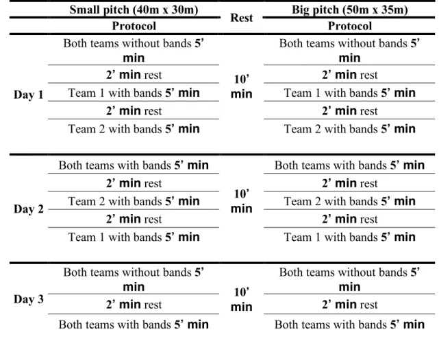
Table 2. Study protocol

Small pitch (40m x 30m)

Rest Big pitch (50m x 35m)

Protocol Protocol

Day 1

Both teams without bands 5’ min

10’ min

2’ min rest 2’ min rest

Team 1 with bands 5’ min Team 1 with bands 5’ min

Day 2

Both teams with bands 5’ min

10’ min

Both teams with bands 5’ min

Day 3

Both teams without bands 5’

min _10’

min

Both teams with bands 5’ min Both teams with bands 5’ min

2.4 Procedures

Before the first day of testing, the players had a familiarization process to the study protocol. This was performed two days before the beginning of the study protocol. This familiarization process was to access the quality of the bands, to see if they would

(26)

sustain the wear and if they would be comfortable for the players to use and for the players to understand the experiment, so they can all be in the same equal state. The first day started with a 25-minute warm-up, composed with low intensity running, limb activation, passes with the ball and dynamic stretching exercises. After the warm-up, the players proceeded to the small pitch to play three matches of 5 minutes each with 2 minutes of rest in between. Then after that the players rested for 10 minutes and played in the big pitch, replicating the same protocol of the small pitch, with three 5 minute matches with 2 minutes rest in between (see Table 2). The second day we followed the same warm-up and after that the players played in the small pitch three matches of 5 minutes with 2’ minutes rest. After a 10 minute rest the players proceeded to the big pitch and replicated the same match conditions as the small pitch (see Table 1). The third day occurred 14 hours after the second day. Due to the tight schedule of the players and coach, we decided to have the less physical demanding day of the protocol for last. With the same warm-up, the player headed to the small pitch and played two 5 minute matches with 2 minutes rest in between. After that they rested for 10 minutes and replicated the protocol in the big pitch, with two 5 minute matches with 2 minutes rest in between.

To keep the work rate of the players high, the coach would often give verbal incentives so they would be encouraged to give their best in each match. One strategy that worked well was to give the players rewards for the winning team. Each session ended with a cool down and a final talk explaining the dates and times for next session.

During the whole protocol, hydration was very important for the players and during the big 10-minute rest, the players would lay down in a shadow or in a cool place with breeze. To monitor the intensity of the protocol we used the RPE scale (see Table 6) (25) to see if they were able to proceed with the protocol, if so the protocol would stop and then reschedule and rethink. The values never overtook 6 in the RPE scale, so the effort was not a fatigue effort by the players, which enabled the experiment to continue with a similar performance throughout.

(27)

2.5 Pitch-positioning derived-variables

For the physical and tactical variables, the coordinates of the players were needed. So, the players’ positional data was captured over time using a 5Hz non-differential global positioning system (SPI-Pro, GPSports, Canberra, ACT, Australia). The devices were placed on the upper back of each player with the respective harness. Latitude and longitude data collected from each individual outfield player were synchronized. If there were any missing data gaps, then they were re-sampled using an interpolation method to guarantee the same length of the time series. The coordinates data gathered was transposed to meters, using the Universal Transverse Mercator (UTM) coordinate system by means of a Matlab routine, and smoothed using a two-points moving average to reduce the tracking error noise (Folgado et al., 2014; Palacios, 2006). The version of Matlab used was Matlab R2014b (MathWorks, Inc., Massachusetts, USA).

Only one position-specific centroid was calculated for each team, and for that was used the dynamic positional data as the mean position from the four field players of each team. The absolute distances from each player to their own team centroid and the opponents’ centroid was calculated as well. Each player is a source of data that contributes to the computation of the team centroid. The dynamical relations between team-specific centroids were performed for both lateral and longitudinal directions (pitch-wide and length, respectively).

The distance covered at different movement speed categories and the game pace (i.e., average speed for each player in each scenario) were measured as physical performance indicators. The following categories were used: walking (0.0 – 7.0 km/h); light jogging (7.1 – 10.0 km/h); faster jogging (10.1 – 13.0 km/h); running (13.1 – 15.0 km/h); sprinting (15.1 – 18.0 km/h); and maximal speed (>18.1 km/h).

Taking into consideration the 2D coordinates retrieved from the pitch, that were used to process the following variables: (i) distance to their own team centroid, expressed by the absolute values (m); (ii) variability in the distance to their own team centroid (CV); (iii) predictability in the distance to their own team centroid, expressed by the approximate entropy (ApEn); (iv) distance to the opponents team centroid, expressed by the absolute values (m); (v) variability in the distance to the opponents team centroid (CV); (vi) predictability in the distance to the opponents team centroid, expressed by the approximate entropy (ApEn).

(28)

ApEn technique was used to assess regularity or predictability of the time series correspondent to the distance between players’ (predictability of the intra-team positioning). Input values for computations were 2.0 to the vector length (m) and 0.2 standard deviations to the tolerance factor (r). The outcome range between 0 and 2 (arbitrary units) and lower values represented more repeatable, regular, predictable and less chaotic sequences of data points (Pincus, 1991).

Effects of pitch area-restrictions during the football matches, dictates that ApEn results express the probability that the configuration of one segment of data in a time

series will allow the prediction of the configuration of another segment of the time series a certain distance apart (Harbourne & Stergiou, 2009). This technique identifies if players’ displacement trajectories express a regular and predictable pattern which may, in turn, provide information regarding their tactical behaviour (Duarte et al., 2013; Gonçalves et al., 2014; Sampaio et al., 2014).

2.6 Statistical analysis

The magnitude-based inferences and precision of estimation was employed aiming to avoid the shortcomings of research approaches supported by the null-hypothesis significance testing (Batterham & Hopkins, 2006). Prior to the scenario comparisons (i.e., without vs with bands and without against with bands vs with against without bands), all processed variables were log-transformed to reduce the non-uniformity of error. A descriptive analysis was performed using mean and standard deviations for each variable (the mean shown is the back-transformed mean of the log transform). The comparisons among game scenarios were assessed via standardized mean differences, computed with pooled variance and respective 90% confidence intervals (Hopkins et al., 2009). Thresholds for effect sizes statistics were 0.2, trivial 0.6, small 1.2, moderate 2.0, large and >2.0, very large (Hopkins et al., 2009). Differences in means for both pairs of scenarios were also expressed and graphically represented in percentage units with 90% confidence limits (CL). The effect was reported as unclear if the CL overlapped the thresholds for smallest worthwhile changes, which were computed from the standardized units multiplied by 0.2. Magnitudes of clear effects were described according to the following scale: 25-75%, possible; 75-95%, likely; 95-99%, very likely; >99%, most likely (Hopkins et al., 2009).

(29)

3. Results

3.1 Physical Performance

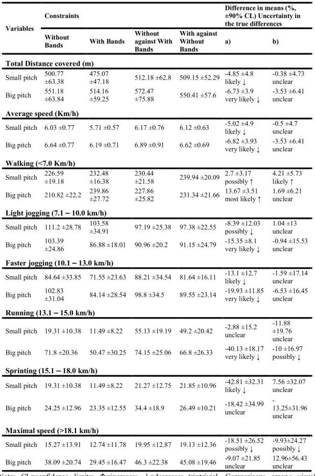
The table 3 shows the results from the descriptive physical analysis, which are the outcome of comparisons among the constraint variables. In the total distance covered showed a likely decrease in both small pitch and big pitch during the constraint of with bands vs without bands. Also, the average speed showed similar results with a likely decrease in the small pitch and a most likely decrease (13.67% ±3.51%) in the big pitch for without vs with bands. During walking intensity, the results show a possibly and most likely increase for both small pitch and big pitch respectably, in the constraint of without vs with bands. As for without against with bands vs with against without bands, showed a likely increase in the small pitch. In light jogging and faster jogging there was an unclear pool of results for without against with bands vs with against without bands but for without vs with bands showed a possibly and likely decrease in light jogging for both small and big pitch respectably, and as well as a likely and very likely decrease (-40.13% ±18.17%) for without vs with bands for both small and big pitch respectably. As for running the only results word mention was a very likely decrease for without vs with bands in the big pitch and a possibly decrease for without against with bands vs with against without bands in the big pitch as well. For the distance covered in sprinting sowed a likely decrease for without against with bands vs with against without bands. The distance covered during maximal speed sowed a possibly decrease for both without vs with bands and without against with bands vs with against without bands, in the small pitch.

(30)

Table 3. Descriptive physical analysis (mean ± SD). Difference in means and uncertainty in the true differences comparisons among the different constraints among both types of field dimensions.

Variables

Constraints

Difference in means (%, ±90% CL) Uncertainty in the true differences Without

Bands With Bands

Without against With Bands With against Without Bands a) b)

Total Distance covered (m)

Small pitch 500.77 _±63.38 475.07 _±47.18 512.18 ±62.8 509.15 ±52.29 -4.85 ±4.8 _{likely ↓} -0.38 ±4.73 _unclear Big pitch 551.18 _±63.84 514.16 _±59.25 572.47 _±75.88 550.41 ±57.6 -6.73 ±3.9 _{very likely ↓} -3.53 ±6.41 _unclear

Average speed (Km/h)

Small pitch 6.03 ±0.77 5.71 ±0.57 6.17 ±0.76 6.12 ±0.63 -5.02 ±4.9 _{likely ↓} -0.5 ±4.7 _unclear Big pitch 6.64 ±0.77 6.19 ±0.71 6.89 ±0.91 6.62 ±0.69 -6.82 ±3.93 _{very likely ↓} -3.53 ±6.41 _unclear

Walking (<7.0 Km/h)

Small pitch 226.59 _±19.18 232.48 _±16.38 230.44 _±21.58 239.94 ±20.09 2.7 ±3.17 _{possibly ↑} 4.21 ±5.73 _{likely ↑} Big pitch 210.82 ±22.2 239.86 _±27.72 227.86 _±25.82 231.34 ±21.66 13.67 ±3.51 _{most likely ↑} 1.69 ±6.21 _unclear

Light jogging (7.1 – 10.0 km/h)

Small pitch 111.2 ±28.78 103.58 _±34.91 97.19 ±25.38 97.38 ±22.55 -8.39 ±12.03 _{possibly ↓} 1.04 ±13 _unclear Big pitch 103.39 _±24.86 86.88 ±18.01 90.96 ±20.2 91.15 ±24.79 -15.35 ±8.1 _{very likely ↓} -0.94 ±15.53 _unclear

Faster jogging (10.1 – 13.0 km/h)

Small pitch 84.64 ±33.85 71.55 ±23.63 88.21 ±34.54 81.64 ±16.11 -13.1 ±12.7 _{likely ↓} -1.59 ±17.14 _unclear Big pitch 102.83 _±31.04 84.14 ±28.54 98.8 ±34.5 89.55 ±23.14 -19.93 ±11.85 _{very likely ↓} -6.53 ±16.45 _unclear

Running (13.1 – 15.0 km/h)

Small pitch 19.31 ±10.38 11.49 ±8.22 55.13 ±19.19 49.2 ±20.42 -2.88 ±15.2 _unclear -11.88 ±19.76 unclear Big pitch 71.8 ±20.36 50.47 ±30.25 74.15 ±25.06 66.8 ±26.33 -40.13 ±18.17 _{very likely ↓} -10 ±16.97 _{possibly ↓}

Sprinting (15.1 – 18.0 km/h)

Small pitch 19.31 ±10.38 11.49 ±8.22 21.27 ±12.75 21.85 ±10.96 -42.81 ±32.31 _{likely ↓} 7.56 ±32.07 _unclear Big pitch 24.25 ±12.96 23.35 ±12.55 34.4 ±18.9 26.49 ±10.21 -18.42 ±34.99 _unclear

-13.25±31.96 unclear

Maximal speed (>18.1 km/h)

Small pitch 15.27 ±13.91 12.74 ±11.78 19.95 ±12.87 19.13 ±12.36 -18.51 ±26.52 _{possibly ↓} -9.93±24.27 _{possibly ↓} Big pitch 38.09 ±20.74 29.45 ±16.47 46.3 ±22.38 45.08 ±19.46 -9.07 ±21.85 _unclear 12.96±56.43 _unclear

Note: CL=confidence limits; ↑=increase; ↓=decrease; tri=trivial. Comparisons among visual constraints: (a) without bands (two teams without bands) vs with bands (two teams with bands); (b) without against with bands (one team without bands playing against other with bands) vs with against without bands (one team with bands playing against other without bands).

(31)

In the figure 1, the trivial differences for the variable of without against with bands vs with against without bands were found in both small pitch and big pitch scenarios. Only the distance covered of walking (<7 Km/h) presented small higher values. As for the variable of without vs with bands, the results of walking (<7 Km/h) showed moderate higher values in the big pitch and small lower values for the small pitch. Regarding total distance covered, average speed, light jogging and faster jogging, showed small/moderate lower values for both small and big pitch. In the results of sprinting (15.1 – 18.0 Km/h) demonstrated small lower values in the small pitch and big pitch. The running speed showed small/moderate lower values for the small pitch and big pitch respectably, regarding the condition of both teams with bands. The maximal speed showed trivial values for both field dimensions, but showed moderate lower values when one team played with the visual occlusion against another without in the small pitch.

(32)

Figure 1. Standardized (Cohen) differences in physical variables according to the two field dimensions (small pitch and big pitch). Error bars indicate uncertainty in the true mean changes with 90% confidence intervals.

Note: Small pitch=40m x 30m; big pitch=50m x 35m. Comparisons among visual constraints: without bands (two teams without bands) vs with bands (two teams with bands); without against with bands (one team without bands playing against other with bands) vs with against without bands (one team with bands playing against other without bands).

(33)

3.2 Tactical Performance

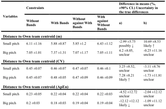
In the table 4 is represented the descriptive tactical analysis of the different constraints. The results were classified as the players distance to the team centroid and the players distance to the opponents’ team centroid. With that the results evaluated the absolute distance, the coefficient of variation and the approximate entropy. The absolute distance results for both distance to own team centroid and opponent centroid showed that in the big pitch was unclear for both conditions. But in the small pitch, regarding the distance to own team centroid, showed a possibly decrease for without vs with bands and a likely increase for without against with bands vs with against without bands. As for the absolute distance to opponent centroid showed a likely trivial difference for without vs with bands and a possibly increase for without against with bands vs with against without bands. Focusing in the coefficient of variation, the results demonstrate a likely decrease in the big pitch for without vs with bands in the distance to own team centroid. As for the distance to opponents’ centroid showed a possibly increase in the small pitch for without vs with bands, and a likely increase in the big pitch for without against with bands vs with against without bands.

Table 4. Descriptive tactical analysis (mean ± SD). Difference in means and uncertainty in the true differences comparisons among the different constraints among both types of field dimensions.

Variables

Constraints

Difference in means (%, ±90% CL) Uncertainty in the true differences Without

Without against With Bands With against Without Bands a) b)

Distance to Own team centroid (m)

Small pitch 6.11 ±1.16 5.88 ±0.87 5.85 ±1.2 6.43 ±1.12 -2.99 ±5.75 _{possibly ↓} 10.69 ±8.53 _{likely ↑} Big pitch 7.05 ±1.01 7.37 ±1.31 7.07 ±1.17 7.05 ±1.11 4.2 ±8.05, _unclear -0.25 ±11.16 _unclear

Distance to Own team centroid (CV)

Small pitch 0.45 ±0.07 0.46 ±0.07 0.47 ±0.07 0.46 ±0.1 3.25 ±8.52, _unclear -3.11 ±8.76 _unclear Big pitch 0.45 ±0.07 0.48 ±0.05 0.47 ±0.09 0.46 ±0.09 7.28 ±8.21 _{likely ↑} -1.73 ±11.81 _unclear

Distance to Own team centroid (ApEn)

Small pitch 0.23 ±0.05 0.22 ±0.04 0.22 ±0.04 0.22 ±0.03 -4.52 ±12.72 _unclear -2.04 ±12.12 _unclear Big pitch 0.2 ±0.03 0.18 ±0.03 0.19 ±0.04 0.19 ±0.04 -12.12 ±12.12 _{likely ↓} -1.09 ±11.12 _unclear

(34)

Distance to Opponent team centroid (m)

Small pitch 6.85 ±1.39 6.76 ±1.3 6.89 ±1.07 7.35 ±1.26 -1.33 ±3.6 _{likely tri} 6.37 ±8.58 _{possibly ↑} Big pitch 8 ±1.39 8.23 ±1.34 7.89 ±0.89 7.84 ±0.99 3.25 ±7.32 _unclear -0.85 ±8.36 _unclear

Distance to Opponent team centroid (CV)

Small pitch 0.45 ±0.11 0.47 ±0.09 0.47 ±0.08 0.46 ±0.1 5.8 ±6.42 _{possibly ↑} -1.81 ±6.47 _unclear Big pitch 0.46 ±0.06 0.5 ±0.07 0.48 ±0.08 0.48 ±0.1 7.7 ±5.97 _{likely ↑} 0.69 ±10.37 _unclear

Distance to Opponent team centroid (ApEn)

Small pitch 0.27 ±0.05 0.24 ±0.04 0.25 ±0.04 0.25 ±0.03 -10.47 ±8.28 _{likely ↓} -0.52 ±8.41 _unclear Big pitch 0.22 ±0.05 0.19 ±0.02 0.22 ±0.04 0.22 ±0.05 -14.52 ±8.71 _{very likely ↓} -5 ±8.63 _unclear

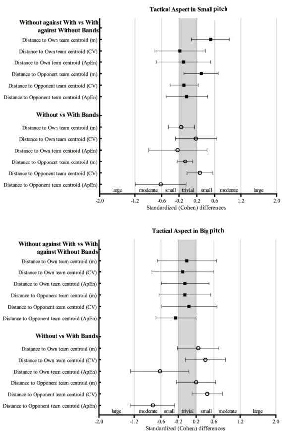
The figure 2 shows the standardized (Cohen) differences in tactical variables. The results display small higher values of the distance to own and opponents’ team centroid for without against with bands vs with against without bands in the small pitch. As for the without vs with bands scenarios showed a small/moderate and moderate lower values of the distance to own and opponents’ team centroid (ApEn) in both small and big pitch respectably. The distance to opponents’ team centroid (CV), showed small higher values for both small and big pitch. When playing in the big pitch the distance to own team centroid (m) and the distance to own team centroid (CV) presented small higher values compared to the small pitch which presented trivial values.

(35)

Figure 2. Standardized (Cohen) differences in tactical variables according to the two field dimensions (small pitch and big pitch). Error bars indicate uncertainty in the true mean changes with 90% confidence intervals.

pitch

(36)

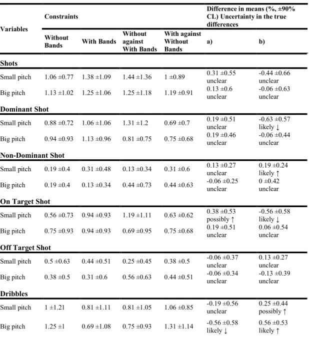
3.3 Technical Performance

The results demonstrating the technical analysis of the experiment, were divided into 4 different main categories: shots, dribbles, passes and touches. Also, the accuracy and the preference of foot used for these categories was gathered. The criteria for shots taken was for every shot taken with the preferred foot of each player was considerate a dominant shot, and if it was on target (including post and bar of the net) was a dominant shot on target. For the dribbles, were counted each time the player attempted to pass the opponent using take-on, dribbles and football skills. If he was successful and passed the opponent it was considered a successful dribble. The category of passes was the total number of passes taken by all players. If the pass arrived to another player of the same team without any interceptions, then the pass was considered successful. And if the pass was taken with the preferred foot, then was considered a dominant pass. The final category was the touches, the total amount of touches that a player took every time he had the ball in his feet. If he touched with the preferred foot, then it counts as a dominant touch.

In the table 5 the results of shots taken showed an unclear difference between the constraints. But when considering non-dominant shots, showed a likely increase for without against with bands vs with against without bands in a small pitch.

As for the data regarding the dribbles, showed a likely decrease and a likely increase in the big pitch for without vs with bands and without against with bands vs with against without bands, respectably. In the small pitch the dribble and success dribble had a possibly increase for without against with bands vs with against without bands. In the success dribble, there was a likely decrease and a possibly increase in the big pitch for without vs with bands and without against with bands vs with against without bands, respectably.

The results of the touches and the dominant touches showed a possibly increase for without vs with bands in the small and big pitch scenarios. As for the non-dominant touches, showed possibly increase for both without vs with bands and without against with bands vs with against without bands in the small pitch. In the bid field occurred a likely increase in non-dominant touches for without vs with bands.

Finally, the data gathered for the passes demonstrates a likely and possibly decrease for without vs with bands in the small and big pitch respectably. Interestingly the use of dominant passes had a likely decrease for without vs with bands in a small pitch. As for the use of non-dominant passes had a likely decrease for without vs with bands in the

(37)

big pitch. And more interesting was the results showed for without against with bands vs with against without bands, which demonstrated that was a likely and possibly increase of non-dominant passes in the small and big pitch scenarios respectably. As for the success of the passes, showed a likely and possibly decrease for without vs with bands in the small and big pitches respectably. The non-success passes showed a likely increase for without against with bands vs with against without bands in the small pitch scenario.

Table 5. Descriptive technical analysis (mean ± SD). Difference in means and uncertainty in the true differences comparisons among the different constraints among both types of field dimensions.

Variables

Constraints Difference in means (%, ±90% CL) Uncertainty in the true differences

Without

Without against With Bands With against Without Bands a) b) Shots

Small pitch 1.06 ±0.77 1.38 ±1.09 1.44 ±1.36 1 ±0.89 0.31 ±0.55 _unclear -0.44 ±0.66 _unclear Big pitch 1.13 ±1.02 1.25 ±1.06 1.25 ±1.18 1.19 ±0.91 0.13 ±0.6 _unclear -0.06 ±0.63 _unclear

Dominant Shot

Small pitch 0.88 ±0.72 1.06 ±1.06 1.31 ±1.2 0.69 ±0.7 0.19 ±0.51 _unclear -0.63 ±0.57 _{likely ↓} Big pitch 0.94 ±0.93 1.13 ±0.96 0.81 ±0.75 0.75 ±0.68 0.19 ±0.46 _unclear -0.06 ±0.44 _unclear

Non-Dominant Shot

Small pitch 0.19 ±0.4 0.31 ±0.48 0.13 ±0.34 0.31 ±0.6 0.13 ±0.27 _unclear 0.19 ±0.24 _{likely ↑} Big pitch 0.19 ±0.4 0.13 ±0.34 0.44 ±0.73 0.44 ±0.63 -0.06 ±0.25 _unclear 0 ±0.42 _unclear

On Target Shot

Small pitch 0.56 ±0.73 0.94 ±0.93 1.19 ±1.11 0.63 ±0.62 0.38 ±0.53 _{possibly ↑} -0.56 ±0.58 _{likely ↓} Big pitch 0.75 ±0.93 0.94 ±0.93 0.69 ±0.95 0.75 ±0.68 0.19 ±0.51 _unclear 0.06 ±0.54 _unclear

Off Target Shot

Small pitch 0.5 ±0.63 0.44 ±0.51 0.25 ±0.45 0.38 ±0.5 -0.06 ±0.37 _unclear 0.13 ±0.27 _unclear Big pitch 0.38 ±0.5 0.31 ±0.6 0.56 ±0.63 0.44 ±0.51 -0.06 ±0.34 _unclear -0.13 ±0.39 _unclear

Dribbles

Small pitch 1 ±1.21 0.81 ±1.11 0.81 ±1.05 1.06 ±0.85 -0.19 ±0.56 _unclear 0.25 ±0.44 _{possibly ↑} Big pitch 1.25 ±1 0.69 ±1.08 0.75 ±0.93 1.31 ±1.14 -0.56 ±0.58 _{likely ↓} 0.56 ±0.53 _{likely ↑}

(38)

Success Dribble

Small pitch 0.69 ±0.95 0.56 ±0.81 0.44 ±0.89 0.75 ±0.86 -0.13 ±0.48 _unclear 0.31 ±0.38 _{possibly ↑} Big pitch 0.81 ±0.83 0.44 ±0.63 0.56 ±0.63 0.88 ±0.89 -0.38 ±0.32 _{likely ↓} 0.31 ±0.41 _{possibly ↑}

Non-Success Dribble

Small pitch 0.31 ±0.48 0.25 ±0.45 0.38 ±0.5 0.31 ±0.48 -0.06 ±0.19 _unclear -0.06 ±0.37 _unclear Big pitch 0.44 ±0.63 0.25 ±0.58 0.19 ±0.4 0.44 ±0.51 -0.19 ±0.4 _unclear 0.25 ±0.25 _{likely ↑}

Touches

Small pitch 12.31 _±6.39 14.63 ±7.09 13.94 ±8.9 16.31 ±8.44 2.31 ±2.16 _{possibly ↑} 2.38 ±5.72 _unclear Big pitch 14.31 _±8.27 16.63 ±8.88 16.06 ±10.47 14.69 ±11.22 2.31 ±3.57 _{possibly ↑} -1.38 ±6.27 _unclear

Dominant Touch

Small pitch 10.06 _±5.25 11.88 ±6.3 10.63 ±7.77 12.25 ±8.01 1.81 ±1.86 _{possibly ↑} 1.63 ±5.14 _unclear Big pitch 12 ±8.05 13.38 ±7.55 13 ±8 11.06 ±8.8 1.38 ±2.98 _{possibly ↑} -1.94 ±5.14 _unclear

Non-Dominant Touch

Small pitch 2.25 ±1.65 2.75 ±1.84 3.31 ±2.12 4.06 ±2.14 0.5 ±0.8 _{possibly ↑} 0.75 ±1.08 _{possibly ↑} Big pitch 2.31 ±1.54 3.25 ±2.24 3.13 ±1.82 3.63 ±2.83 0.94 ±0.9 _{likely ↑} 0.5 ±1.43 _unclear

Passes

Small pitch 6.63 ±2.83 5.19 ±2.86 4.63 ±2.25 4.81 ±2.71 -1.44 ±1.1 _{likely ↓} 0.19 ±1.7 _unclear Big pitch 5.31 ±2.24 4.63 ±2.16 4.69 ±1.99 4.63 ±2.83 -0.69 ±1.05 _{possibly ↓} -0.06 ±1.7 _unclear

Dominant Pass

Small pitch 5.88 ±2.85 4.5 ±2.31 4.06 ±2.14 4.06 ±2.84 -1.38 ±1.1 _{likely ↓} 0 ±1.82 _unclear Big pitch 4.69 ±2.18 4.31 ±2.27 4.19 ±2.14 3.69 ±2.73 -0.38 ±1 _unclear -0.5 ±1.78 _unclear

Non-Dominant Pass

Small pitch 0.75 ±0.93 0.69 ±0.95 0.56 ±0.63 0.75 ±0.58 -0.06 ±0.49 _unclear 0.19 ±0.29 _{possibly ↑} Big pitch 0.63 ±0.72 0.31 ±0.48 0.5 ±0.82 0.94 ±0.68 -0.31 ±0.38 _{likely ↓} 0.44 ±0.48 _{likely ↑}

Success Pass

Small pitch 5.75 ±2.05 4.69 ±2.33 4.13 ±2.22 3.69 ±2.65 -1.06 ±0.87 _{likely ↓} -0.44 ±1.75 _unclear Big pitch 4.44 ±2.19 3.94 ±1.95 4 ±1.86 4.13 ±2.83 -0.5 ±0.95 _{possibly ↓} 0.13 ±1.67 _unclear

Non-Success Pass

Small pitch 0.88 ±1.36 0.5 ±0.73 0.5 ±0.63 1.13 ±0.89 -0.38 ±0.64 _unclear 0.63 ±0.45 _{likely ↑} Big pitch 0.94 ±1.12 0.69 ±0.79 0.69 ±0.6 0.5 ±0.73 -0.25 ±0.57 _unclear -0.19 ±0.46 _unclear

(39)

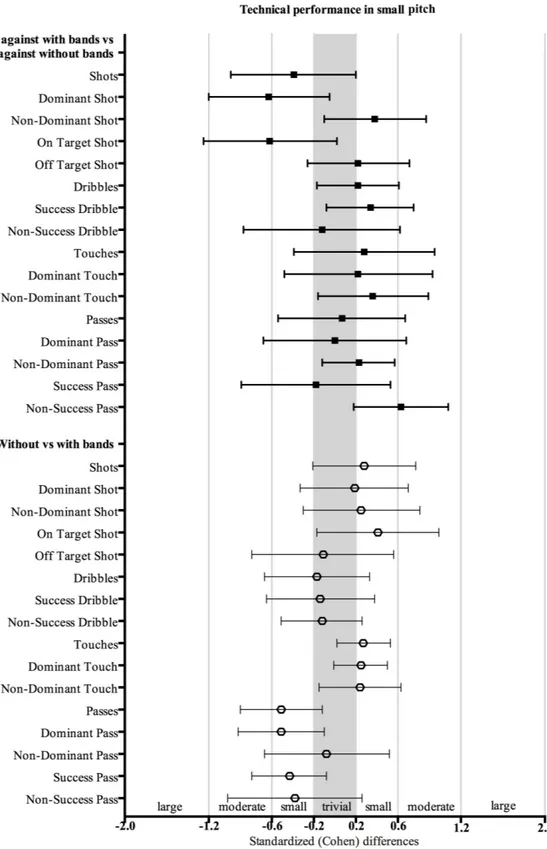
The figure 3 display the standardized (Cohen) differences in technical variables. For without against with bands vs with against without bands the results showed moderate lower values in the dominant shots and on target shots taken in the small pitch. The non-success pass presented a moderate higher value in the small pitch. In the big pitch, there was a moderate higher value for the non-dominant pass.

As for the without vs with bands, presented small higher values in the non-dominant touch for both small and big pitch. Also presented small lower values for success and non-success passes in both small and big pitch. The results of dribbles also shown smaller values without bands in the big pitch, as oppose to the small pitch where the values present no changes.

The non-dominant pass presented lower smaller values for players without bands and higher smaller values for players with bands playing against without bands, for both small and big pitch.

(40)

Figure 3. Standardized (Cohen) differences in technical variables according to the two field dimensions (small pitch and big pitch). Error bars indicate uncertainty in the true mean changes with 90% confidence intervals.

(41)