Wine metrics : revealing the volatile molecular feature responsible for the wine like aroma

WINE METRICS : REVEALING THE VOLATILE MOLECULAR FEATURE

RESPONSIBLE FOR THE WINE LIKE AROMA

Thesis presented to Escola Superior de Biotecnologia of the Universidade

Católica Portuguesa to fulfill the requirements of Master of Science degree in

Food Engineering

by

João Manuel Tomé Domingues

Place: Escola Superior de Biotecnologia – Universidade Católica Portuguesa Supervision: Doutor António César da Silva Ferreira

III

Resumo

O vinho é uma matriz complexa composta por uma variedade de aromas provenientes das diferentes interações dos seus variados compostos. Aroma é geralmente associado a compostos voláteis, que resultam da fermentação alcoólica de acordo com a levedura utilizada e condições utilizadas. A grande concorrência do sector está levar os produtores a compreender melhor as expectativas e preferências dos seus consumidores. A motivação desta tese vai ao encontro de uma ferramenta para compreender o aroma “tipo-vinho” levando à seleção de estirpes de S. cerevisiae de acordo com o padrão de voláteis em função dos consumidores. Este trabalho irá fornecer informações sobre a conexão entre o metabolismo da fermentação do vinho e a percepção do aroma vínico.

Neste contexto, foram realizadas 3 réplicas de 4 fermentações em um meio sintético, usando diferentes estirpes de levedura em cada fermentação (3 estirpes vínicas: QA23, VL1, ZA e 1 estirpe de cachaça: L328). Os perfis metabólicos das fermentações foram obtidos através de cromatografia gasosa ligada a um detetor de ionização por chama (GC-FID), espectrometria de massa (GC-MS) e cromatografia líquida de alto desempenho (HPLC) de modo a quantificar os compostos. Um estudo sensorial foi usado para avaliar se os consumidores reconheciam o aroma “tipo-vinho” no decorrer das fermentações. Esta estratégia direcionada em conjunto com uma análise não direcionada usando técnicas de análise multivariada como: decomposição singular do valor (SVD) e análise hierárquica de Agrupamentos (HCA), revelou que o aroma “tipo-vinho” das fermentações está relacionada com acetaldeído, acetato de hexilo e ésteres etílicos. A estirpe L328 revelou-se a que apresenta melhores resultados sensoriais e melhor correlação com os compostos responsáveis pelo aroma “tipo-vinho”. Uma análise supervisionada, nomeadamente PLS-R, permitiu a construção de um modelo que prevê os resultados (R2 = 0.8)) sensoriais do aroma “tipo-vinho” pelo padrão aromático. Por fim uma estratégia não direcionada foi usada com os dados de GC-MS pré-processados e análise por SVD. Este método demonstrou distinguir estirpes baseadas na evolução metabólica durante a fermentação, L328 e QA23 revelaram ser facilmente distinguíveis das restantes.

No decorrer desta tese foram utilizadas estratégias de quimiometria e bioinformática para o estudo metabólico de fermentações e a possibilidade de uma pré-seleção das estirpes de acordo as características do produto final.

V

Abstract

Wine represents a variety of aromas that stem from a complex, completely non-linear system of interactions among many hundreds of compounds. Aroma is usually associated with odorous or volatile compounds that result from fermentation. Yeast strain and fermentation conditions are claimed to be the most important factors influencing the aromas produced in wine. The fierce competition is forcing wine producers to understand better the expectations and preferences of their target market so they can produce wines accordingly. The motivation of this thesis is in the line with a tool for yeast strains selection according with the volatiles output giving a better acceptance by the consumers. This work provided insights about the connection between the wine fermentation metabolism and the product “wine-like” aroma perception.

In this context were performed 3 replicas of 4 fermentations of a synthetic grape juice with a different S. cerevisae strain on each (3 wine strains: QA23, VL1, ZA and 1 cachaça strain: L328). The metabolic profiles of fermentations were obtained using gas chromatography attached to a flame ionization detector (GC-FID) or to mass spectrometry (GC-MS) and High Performance Liquid Chromatography (HPLC). A sensorial study also was used in order to evaluate the recognition of a “wine-like” aroma. This target approach coupled with unsupervised analysis, namely Singular Value Decomposition (SVD) and Hierarchical Cluster Analysis (HCA), revealed that the “wine-like” aroma key odorants are acetaldehyde, hexyl acetate and ethyl esters. L328 revealed to be the strain with better scores and correlation with the sensorial analysis scores of “wine-like”. A supervised analysis, Partial least squares regression (PLS-R) model, allowed the prediction (R2 = 0.8) of the “wine-like” scores of the samples during fermentation process. Finally, an untargeted metabolomic approach combining GC-MS data preprocessing with SVD was able to distinguish strains based on their metabolic profiles evolution during the fermentation time. L328 and QA23 strains revealed to be easily distinguished from each other and from the couple ZA and VL1.

In conclusion this study demonstrated the potential of the use of chemometrics and bioinformatics approaches was explored in the characterization, prediction and classification of metabolic profiles from fermentations and the possibility of selection of the yeast strain

VII

Acknowledgments

I wish to express my sincere gratitude and appreciation to all persons that contributed to this achievement:

Dr. António César Ferreira, who as my supervisor, provided guidance, advice, much needed encouragement, in addition to the critical evaluation of this manuscript.

All my friends and colleagues at the Universidade Católica Portuguesa, that during these years helped me, in special to Ana Rita Monforte for her indispensable presence.

IX Contents RESUMO ... III ABSTRACT ... V ACKNOWLEDGMENTS ... VII CONTENTS ... IX LIST OF FIGURES ... XI LIST OF TABLES ... XIII LIST OF ABBREVIATIONS ... XV

1. INTRODUCTION ... 17

1.1. WINE AROMA AND FLAVOR ... 18

1.2. YEAST AND ITS IMPORTANCE TO WINE AROMA ... 19

1.3. SUGAR AND ETHANOL ... 20

1.4. VOLATILES SYNTHESIS ... 20 1.4.1. Higher alcohols ... 23 1.4.2. Volatile Acids ... 23 1.4.3. Esters ... 24 1.5. METABOLOMICS ... 25 1.5.1. Analytical techniques ... 25 1.4.1.1. Gas chromatography ... 26 1.4.1.2. Liquid chromatography ... 27

1.5.2. Metabolomics: signal process techniques ... 28

1.5.2.1. Unsupervised multivariate method: Cluster Analysis ... 28

1.4.2.2. Unsupervised multivariate method: Singular Value Decomposition (SVD) ... 29

1.4.2.3. Supervised multivariate method: Partial least squares regression (PLS-R) ... 30

2. MATERIAL AND METHODS ... 31

2.1. REAGENTS ... 31

2.2. STRAIN, MEDIA AND CULTURE CONDITIONS ... 31

2.3. GROWTH MEASUREMENT ... 31

2.4. SENSORIAL ANALYSIS ... 31

2.5. ANALYTICAL PROCEDURES ... 32

2.5.1. Analytical methods – HPLC ... 32

2.5.2. Analytical methods – GC-FID ... 32

2.5.3. Analytical methods – GC-MS ... 33

2.6. DATA ANALYSIS ... 33

X

2.6.2. Multivariate Analysis ... 34

3. RESULTS AND DISCUSSION ... 35

3.1. FERMENTATION KINETICS ... 35 3.2. SENSORY ANALYSIS ... 37 3.3. VOLATILES FORMATION ... 38 3.3.1. Targeted approach ... 39 3.4.2.3. Unsupervised Techniques ... 42 3.4.2.3. Supervised Techniques ... 48 3.3.2. Untargeted approach ... 52 4. CONCLUSION ... 61 5. FUTURE WORK ... 63 6. REFERENCES ... 65

XI

List of Figures

Figure 1. Illustration of yeast metabolism

Figure 2. Glycolysis pathway in the alcoholic fermentation Figure 3. Example of a MS three-dimensional graphic

Figure 4. CO2 release during fermentation. Values are the average of three biological repeats

± standard deviation. L328 (cachaça strain), QA23 and VL1 (commercial wine strain) and ZA (laboratory wine strain).

Figure 5. Fermentation kinetics of the four yeast strains used in this study: glucose (A) and

fructose (B) consumption, glycerol (C) and ethanol (D) formation. All y-axis are in grams per litter and refer to extracellular metabolite concentrations in the synthetic mediums. Values are the average of three biological repeats ± standard deviation.

Figure 6. Percentage of the panelists that associate the fermentation aroma with the

“wine-like” aroma. Values are the average of three biological repeats ± standard deviation.

Figure 7. Comparison of Ethyl butanoate production rates by concentration of CO2(A) with

by time(B).

Figure 8. Principal component analysis score plot of PC1, PC2 and PC3 projected against

fermentation time (A) and CO2 release (B).

Figure 9.Singular value decomposition plot: PC1 vs. PC2 and PC1 vs. PC3 of the normalized

volatile data obtained combined with the “wine-like”

Figure 10. Principal component analysis: PC1 vs. PC4 of the normalized volatile data

obtained combined with the “wine-like” feature.

Figure 11. Cluster analysis of the fermentations data combined with “wine-like” feature. Figure 12. PLS-R method for “wine-like” feature for prediction in fermentation.

XII

Figure 14. PLS-R method for “wine-like” feature for prediction in fermentation before 142

hours (maximum wine-like)

Figure 15. Distribution of volatiles compounds in accordance with PLS model until 142

hours.

Figure 16. Raw data alignment

Figure 17. Zoom-in of the alignment of raw data.

Figure 18. Singular value decomposition: PC1 vs. PC2 using an untargeted approach.

Figure 19.Chromatogram of GC-MS raw data (metabolic data) vs PC 1.

Figure 20. Illustration of the effect of time in PC1 scores (untargeted). Figure 21.. Singular value decomposition: loadings plot PC2.

Figure 22.Singular value decomposition: PC1 vs. PC3 using an untargeted approach.

XIII

List of Tables

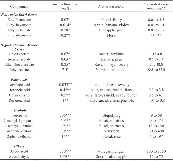
Table 1. Aroma compounds commonly found in wines with important influence in sensorial

perception

Table 2. Average concentrations of the measured compounds of all replicas ± standard

deviation in the last point of fermentation.

Table 3. Average concentrations of the measured compounds of all replicas ± standard

deviation in the point of fermentation with more wine-like (142 hours).

Table 4. Validation statistics of the performance of PLS method on prediction of "wine-like"

feature.

Table 5. Validation statistics of the performance of PLS method on prediction of "wine-like"

XV

List of Abbreviations

Acetyl-CoA Acetyl coenzyme A

ANOVA Analysis of Variance

ATP Adenosine Triphosphate

CDF Common Data Form

FID Flame Ionization Detector

GC Gas Chromatography

GC-FID Gas Chromatography – Flame Ionization Detector

GC-MS Gas Chromatography - Mass Spectrometry

H2S Hydrogen Sulfide

HPLC High Performance Liquid Chromatography

IR Infrared

min minutes

MS Mass Spectrometry

MVA Multivariate Analysis

MVDA Multivariate Data Analysis

NAD Nicotinamide Adenine Dinucleotide

PC1 First Principal Component

PC2 Second Principal Component

PC3 Third Principal Component

PC4 Fourth Principal Component

PLS Partial Least Squares

PLS-R Partial Least Squares Regression

R2 Coefficient of determination

RMSEC Root Mean Square Error of Calibration

RMSECV Root Mean Square Error of Cross Validation

RT Retention Time

SGJ Synthetic Grape Juice

SPME Solid Phase Microextration

SVD Singular Value Decomposition

17

1. Introduction

The ancients explained the boiling during fermentation (from the Latin fervere, to boil) as a reaction between substances that come into contact with each other during crushing [1]. In the XVII century, Antonie van Leeuwenhoek analyzed yeast in beer wort using a microscope, but the relationship between yeast and alcoholic fermentation wasn´t establish. Only in the end of the XVIII century Lavoisier started the study of yeasts and alcoholic fermentation [2], when with his studies in wine and beer gave a true credibility to the viewpoint of alcoholic fermentation. His studies showed that the yeasts responsible for spontaneous fermentation of grape must came from the surface of the grape [2]. He even conceived the view that the strain of the yeast could influence the characteristics of the wine and that the yeast during fermentation also produced other products such as glycerol in addition to alcohol and carbon dioxide.

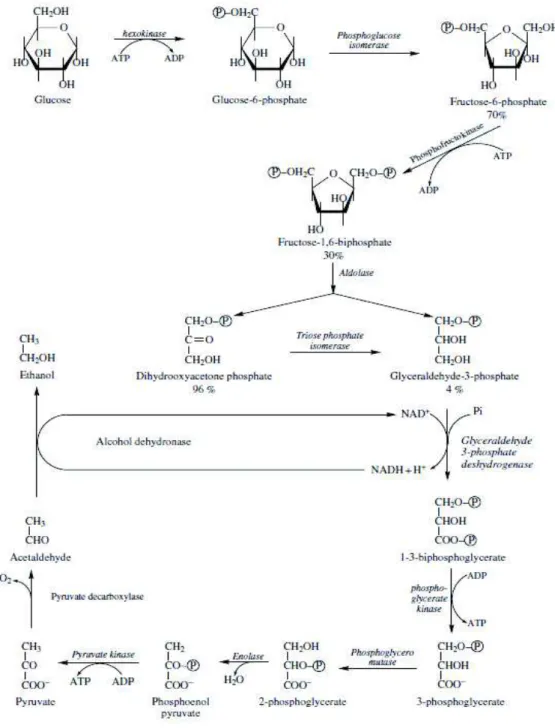
Depending on aerobic conditions, yeast can degrade sugars using two metabolic pathways: alcoholic fermentation (Figure 1) and respiration [3]. Both start with the same process, glycolysis, responsible of the transformation of sugars into pyruvate with the formation of adenosine triphosphate (ATP) [3]. Fermentation produces nicotinamide adenine dinucleotide (NAD+) by the decarboxylation of pyruvate into acetaldehyde, itself reduced to form ethanol [3]. Pyruvate can also be used in other secondary metabolic pathways, to form many volatile compounds such as higher alcohols, esters and fatty acids[3].

18

1.1. Wine Aroma and Flavor

Knowledge of wine flavor is connected with the developments in analytical chemistry. In the past, only the major wine components (ethanol, organic acids and sugar) were quantified in wines. The appearance of new analytical techniques, in particularly the development of gas chromatography, allowed the scientists to discover the uncharted compounds of the wine [2]. At this date more than 1300 volatile compounds have already been identified in beverages [4]. The aim of the analyses shifted from identification and quantification of new compounds toward developing dynamic analytical techniques that can show the relation between volatile composition and sensory properties. The expression “aroma” refers to “a strong, pleasant smells, usually from food or drink" (Definition of aroma from the Cambridge Advanced Learner’s Dictionary & Thesaurus, Cambridge University Press). In oenology, aroma means all fragrances of young wines, while the acquired odor during aging is called bouquet [5]. From the consumer’s point of view flavor and aroma in the wine is an essential factor in making a purchasing decision [6]. The tangled flavor of wine is derived from many sources, such as grape, yeast, microbial fermentations and post-fermentation treatments such as oak storage and bottle aging[5].

The most basic “wine-like” feature is the human sensorial experience of realizing that “it smells like wine”, hence a pattern recognition event. Humans generally struggle with identifying the components of mixture, even when they are able to identify the components alone, the difficult level gets higher as the complexity increases.

The wine industry has come to realize that today’s consumer’s vote with their wallets for those wines that offer a pleasurable and recognizable “sensory experience”. The wine industry’s challenge is to offer these sentiments to the consumer and produce products with superior quality for the target-market. The evolution of wine industry is forcing producers to understand the expectations and preferences of their consumers and try to offer them the wines they desire [6].

19

1.2.

Yeast and its importance to wine aroma

Today there are a vast number of selected commercial yeast strains capable to realize fermentation to optimize a distinctive character to the wine influencing the aroma by having a different impact in the production of volatiles [7, 8], thus the ability to choose the right yeast strain that produce a wine with the characteristics that the consumers want is really important. These differences are a consequence of the differential ability of wine yeast strains in releasing volatile compounds from the grape precursors and the differential ability to synthesize de novo yeast-derived volatile compounds[9].

With the knowledge about the physiology of genetic reference strains it is possible produce industrial yeast toward practical goals [1].

20

1.3. Sugar and Ethanol

Ethanol is the main volatile compound of wine. It is produced by the Saccharomyces

cerevisiae during catabolism of glucose and fructose (Figure 1 and figure 2) [10]. In the end

of the fermentation the ethanol concentration will depend on the initial concentration of sugars in the must and on the winemaking techniques[3]. Saccharomyces cerevisae is considered to be glucophilic, this means that it will have preference for glucose over fructose. This preference is related to the yeast strain so the discrepancy between glucose and fructose consumption is not a fixed parameter[11].

The presence of ethanol is essential to enhance the sensory attributes of other wine components. Excessive ethanol, however, can produce a perceived ‘hotness’ and mask the overall aroma of the wine [6].

Nitrogen also play a central role in structure and function, and most organisms have elaborate control mechanisms to provide a constant supply of nitrogen[12]. Most of the nitrogen used by yeast comes from ammonia, asparagine, glutamine and glutamate, when these nitrogen sources are absent or in low concentrations (which can limit yeast growth) other sources such as amino acids and peptides are used[11]. Amino acids play an important role in winemaking process, their catabolism result into a range of volatile and non-volatile compounds with impact in the organoleptic qualities of wine[13].

1.4. Volatiles Synthesis

The volatile compounds formed during fermentation have a big impact on the flavor of wines, but there are cases where the concentrations are below of the humans’ sensory thresholds and rarely have an impact on overall wine flavor [4]. The basic aroma of wine, however, can be attributed to four esters: (ethyl acetate, isoamyl acetate, ethyl caproate and caprylate), two alcohols (isobutyl, isoamyl) and acetaldehyde [14]. The vast majority of the other compounds typically function to modify the basic odor. The fermentation-derived aroma compounds found in the highest quantities include propanol, 3-methyl-butanol, 2-methyl-butanol and 2-phenylethanol, which collectively account for near half of the total volatiles [14].

21

22

Table 1. Aroma compounds commonly found in wines with important influence in sensorial perception (adapted from

Swiegers et al. 2005). Compounds !! "#$%&!'(#)*($+,! -%./01! "#$%&!,)*2#34'$#! 5$62)6'#&'3$6!36! 736)!-%./01! !!

Fatty acids Ethyl Esters

! ! ! !

Ethyl butanoate

! 0.02* Floral, fruity 898:!'$!:9;!

Ethyl hexanoate

! 0.014* Apple, banana, violets 898<!'$!<9=!

Ethyl octanoate

! 0.58* Pineapple, pear 898>!'$!<9;!

Ethyl decanoate

! 0.2** Floral 8!'$!?9:!

! ! ! ! !

Higher Alcohols Acetate

Esters ! ! ! ! Hexyl acetate ! 0.67* sweet, perfume 8!'$!=9;! Isoamyl acetate ! 0.03* Banana, pear 89:!'$!<9=! Ethyl phenylacetate

! 0.25* Rose, honey, flowery 8!'$!:;9>!

Ethyl acetate

! 7.5* Varnish, nail polish ??9>!'$!@<9>!

! ! ! ! !

Fatty acids

! ! ! !

Isovaleric acid

! 0.033** rancid, cheese, sweaty !

Hexanoic acid

! 0.42** sour, cheese, rancid, fatty 0.9 to 3.8

Octanoic acid

! 0.5** oily, fatty, rancid, soapy, butter 0.6 to 4.7

Decanoic acid

! 1** fatty, rancid, citrus, phenolic 0.06 to 0.8

! ! ! ! ! Alcohols ! ! ! ! 1-propanol ! 306*** Stupefying 9 to 68 2-methyl-1-propanol ! 40*** Fusel, spiritous 9 to 174 2-methyl-1-butanol ! 40*** Fusel, spiritous 15 to 150 3-methyl-1-butanol ! 30*** Marzipan 60 to 490 2-phenylethanol ! 14** Floral, rose 4 to 197 ! ! ! ! ! Others ! ! ! ! Acetic Acid ! 280*** Vinegar, pungent 100 to 1150

Acetaldehyde !! 100*** Sour, bruised apple 10 to 75

* red wine dearomatised (Pineau, 2007); ** hydro-alcoholic solution (10% v/v ethanol at pH 3.5 + tartaric acid); *** synthetic wine (11% v/v ethanol, 7 g/L glycerol, 5 g/L tartaric acid, pH 3.4);

23 1.4.1. Higher alcohols

The higher alcohols (also known as fusel alcohols) are secondary metabolites but represent the larger group of aromatic compounds produced by the yeast during fermentation[4]. The impact of this group on the wine aroma can be positive or negative; it can give fruity characters at optimal levels but at excessive concentrations can result in a strong, pungent smell and taste [15]. The higher alcohols source is the amino acids usually present in the grape. Yeast can excrete ketonic acid from the deamination of amino acids (the precursors for higher alcohols that can be found in grape must or produced by the yeast in de novo synthesis using ammonium) in the Ehrlich Reaction, so the final concentration of higher alcohols is direct linked to the concentration of amino acids in the medium [7]. For example 3-metil-1-butanol, 2-metil-1-butanol and 2-metil-1-propanol are synthesized by leucine, isoleucine and valine, respectively [16]. There is also on other way for the synthesis of higher alcohols involving the sugars metabolism, which is connected later to the Ehrlich reaction. The preferential path is from the amino acids, representing the source of about 65% of the final higher alcohols [6]. The fusel alcohols found in the largest quantity in wine are 1-propanol, 2-methyl-1-propanol (isobutyl alcohol), 2-methyl-1-butanol, and 3-methyl-1-butanol (isoamyl alcohol). Quantitatively, isoamyl alcohol generally accounts for more than 50% of all fusel alcohol fractions [14].

1.4.2. Volatile Acids

Yeast metabolism also is responsible for the production of saturated and unsaturated acids present in the wine. The composition of the acids in wine is mostly acetic acid, around 90% [17], the other 10% is mostly short and medium chain acids. These last groups of acids are from the fatty acid metabolism and are rather considered as products intermediates than as end products. Their impact on the aroma is relatively low, but in the other hand, are the precursors of a very important aromatic compound: ethyl esters[17].

24 1.4.3. Esters

Esters are, like the higher alcohols, the most abundant volatiles compounds in wine. This compounds produced by the yeast during fermentation can have a significant impact on the fruity flavors in the final product [4]. As the length of the carbon chain increases fruity odors tend to become soft [14]. The majority of these compounds usually are synthesized by the yeast metabolism, using the lipid and acetyl-CoA metabolism, but some can be produced by grape precursors present in the must [18]. The two big groups of Esters are acetate esters and ethyl esters, the first result from the reaction between acetic acid and the corresponding higher alcohol. Ethyl esters are synthesized from ethanol and the “fatty” acid corresponding [19]. Ethyl esters are found in the largest quantities while acetates, though in less quantity, contribute to some of the intensity and quality of wine aroma. This type of esters are more volatile when compared to other aroma compounds, hence these compounds are partially transferred onto the carbon dioxide produced during the fermentation and can easily swept away [14].

25

1.5. Metabolomics

Metabolomics has been defined as a comprehensive view of the metabolites present in samples. Metabolomic analyses have been generally classified as targeted or untargeted. Targeted analyses focus on specific group of metabolites, which requires in most cases the identification and quantification of metabolites. This type of analyses is important for study the behavior of the group of metabolites under defined conditions, and it is required a high level of purification in the extraction and analyses of the metabolites in study. In the other hand, untargeted analyses has the objective on the detection of all the groups of metabolites possible to acquire biological fingerprints [20].

Metabolomic studies also can be classified as discriminative, informative and predictive, which depends the aim of the analysis. Discriminative analyses have been defined to search differences between sample groups without creating statistical models and know what is causing those differences. This is achieved by the use of multivariate data analysis (MVDA) techniques, being singular value decomposition (SVD) the most used tool [21].

Informative metabolic analysis have the objective to identify and quantify of target or untarget metabolites to obtain sample intrinsic information, such as possible pathways, discovery of biomarkers and creation metabolites databases [22]. For last, predictive analysis which uses statistical models based on metabolites profile to create a tool to predict a variable that is difficult to quantify by other process. These models are usually produced by partial least square (PLS) regression.

The analysis of metabolomics data is perhaps the most challenging and time consuming step in the processing pipeline, so it is necessary to select the right statistical techniques because of high data dimensions [23].

1.5.1. Analytical techniques

It is impossible to use a single analytical technique to cover the entire tier of the wine metabolome, so it is necessary the use of complementary analytical platforms to improve the coverage and identification ability [24].

26 multichannel. Single-channel detectors (FID, HPLC and FTIR) produce a single value for each time sample of the chromatogram, while multichannel detectors (such MS) produce multiple values for each time sample.

1.4.1.1. Gas chromatography

- Gas chromatography – Flame Ionization Detector (GC-FID)

One of the most used methods in any analytical laboratory is Gas Chromatography with Flame Ionization Detection (GC-FID). After the separation of the metabolites in the GC column the FID measures the electrical current generated by burning carbon in the sample, thus making the most sensitive and universal detection method for practically all organic compounds. It is resistant to small fluctuations of gas flow and it is insensitive to gas impurities [25, 26].

- Gas chromatography – Mass Spectrometry (GC-MS)

Gas chromatography attached to mass spectrometry (GC-MS) is based on separation of metabolites by applying heat until they reach their boiling point, fly through the GC column, and reach the detector (MS). In the GC column, metabolites are separated because of their different boiling point and partitioning coefficients between mobile face (GC carrier gas) and stationary phase (GC column). In the end of the GC column is an ionization chamber of a mass spectrometer where eluted metabolite will be ionized by a beam of electrons. Resulted ions further travel through the mass analyzer where ions are separated based on their mass to charge ratio (m/z) and finally reaches the detector. The resolution of the metabolites analysis depends on the GC column separation and on scan speed of the mass spectrometer [27]. The MS detector is a multi-channel which records several parallel signals for each time point resulting in a two dimensional dataset (figure 3).

One of the main challenges of GC-MS metabolomics, which is mostly solved, is processing of the complex data and extraction of relevant information about it. In GC-MS, metabolites can be identified by comparing their retention time/indices and characteristic fragmentation pattern of their mass spectra with databases [27] .

27

Figure 3. Example of a MS three-dimensional graphic (source Bahromovich, 2013 [27])

1.4.1.2. Liquid chromatography

Liquid Chromatography is a chromatographic technique based on the separation of the target compounds contained on the liquid mobile phase using the different interactions between them and the stationary phase[24]. Is a technique used for the separation of macromolecules and ionic species, such as amino acids, polysaccharides and plant or animals metabolites[28]. -High Performance Liquid Chromatography (HPLC)

The use of High Performance Liquid Chromatography (HPLC) seems to be the most suitable for simultaneous analysis of sugars, acids and alcohol in fermentation samples [29].

For metabolomics with the application of this analytical procedures it is necessary three big steps: sample preparation, data acquisition (this first two step are very important for the quality of the obtain data, which will have a good impact on the last step), and data analysis (the right selection of the method will facilitate extraction of the metabolic knowledge)[24].

28

1.5.2. Metabolomics: signal process techniques

There is more than one type of multivariate data analysis techniques, to know how to choose the right on depends on the answer the scientist wants to obtain out of the data analysis. In this work it was used multivariate analysis based on so called projection methods [30]. This projection approach is mostly used to summarizing and visualizing a data set, multivariate classification and discriminate analysis and finding quantitative relationships among the variables.

Target and untarget metabolomics can also be divided in two major categories: unsupervised and supervised techniques. Unsupervised classification is where the outcomes are based on the type of analysis of data without the user providing sample classes [31]. This classification determines which samples are related and groups them into classes (SVD and cluster analysis) [32]. Supervised classification is where the scientist can select sample characteristics that representative of specific classes and then direct the algorithm to use these references for the classification in the samples (such as PLS) [31].

1.5.2.1. Unsupervised multivariate method: Cluster Analysis

Clustering is an important data-mining problem with a wide variety of applications. It is an unsupervised technique for MVA that separate items to automatically created groups based on a degree of similarity between groups (clusters) [33] usually represented as a vector of measurements, or a point in a multidimensional space.

Clustering is mostly useful in situations like exploratory pattern analysis, grouping, decision making and machine learning situations [34]. The big concerning about cluster analysis is that all clustering algorithms will, when presented with data, produce cluster, even if the data contain cluster or not [34]. So the data domain and the expectation of cluster are very important when we want to use this type of tool.

The most common algorithm used is Hierarchical cluster analysis (HCA), in these method hierarchies of subspaces clusters can be discovered, this means, the information of a lower-dimensional cluster is implanted within a higher-lower-dimensional one. The result is a dendrogram (correlation tree) that represent the relative similarities and differences among objects. When

29 performing cluster analysis of multivariate data with different families of compounds, because of complex metabolic pathway it is expected that members of the same organic group or synthesis pathway will cluster [35].

The aim of cluster analysis is to help understanding the data generated or to validate the results obtained from other methods.

1.4.2.2. Unsupervised multivariate method: Singular Value Decomposition (SVD)

SVD is a powerful tool in matrix computation and analysis such as matrix approximation. This technique of data processing has the advantage of reducing the dimensionality of the data set while retaining the important information hidden in the matrix. This can be done by mapping the raw data set onto a reduced orthogonal space assigned in such a manner as to account for most of the original data set’s variability [36] [37]. SVD is made of score and loading plots, score plots contains information about the samples, which are described in terms of theirs projection onto principal components, the loading plots contain information about the variables which are also described in terms of their projection onto principal components.

SVD is based on a theorem from linear algebra which says that a rectangular matrix A can be broken down into the product of three matrices, an orthogonal matrix U, a diagonal matrix S, and the transpose of an orthogonal matrix V (equation 1). Hence the diagonal elements of S are singular values (!) of A and the columns of U and of V are left (u) and right (v) singular vectors of A (equation 2), respectively.

A = USV

A v =

!"u

A

u = !"v

Basically, the aim of a SVD is taking a high dimensional, highly variable set of data points and reducing it to a lower dimensional space that exposes the substructure of the raw data more clearly and orders it from most variation to the least [38]. This means the original data is decomposed into linearly independent components, which are in some way an abstraction from without the noisy correlations found the raw data to sets of values that best approximate

30 the underlying structure of the dataset. SVD is a useful tool for signal processing and pattern recognition in high data dimensions.

1.4.2.3. Supervised multivariate method: Partial least squares regression

(PLS-R)

The aim of a regression analysis is to construct a model, also referred to as a calibration model that connects information in a set of measurements to some desired property, this means to predict the independent variable matrix Y from the dependent variable matrix X and describe their common structure [30].

Partial least squares (PLS) is a chemometric technique used when the explaining variables (predictor variables) are highly correlated. It produces an orthonormal sequence of latent components from the explaining variables, which have maximal covariance with the response variable [39]. The main purpose of PLS regression in this study was to build linear calibration models that enable prediction of desired characteristics. The statistical indicators used to evaluate the model are bias, root mean square error of cross validation (RMSECV), root mean square error of calibration (RMSEC) and coefficient of determination (R2

)

Bias refers to the mean difference between the predicted and the measured reference values for all the samples in a validation set. It is a measure of the overall accuracy of a prediction model and is expressed in the same unit as the original reference data. RMSECV describes the predictive accuracy of the calibration model in relation to the reference data. RMSEC gives an indication of the average prediction error obtained for several samples. Coefficient of determination (R2

)

31

2. Material and Methods

2.1.

Reagents

Chemicals and standards were obtained from Sigma-Aldrich, USA (a high-purity grade, >99.0%). Anhydrous sodium sulfate was obtained from Merck, Darmstadt, Germany.

2.2.

Strain, media and culture conditions

The two commercial wine strains used in this study were S.cerevisiae QA23 (Lallemand, Montreal, Canada) and Zymaflore VL1 (Laffort, Bordeux, France), a cachaça strain codified as L328 and a laboratory wine strain from Douro region, Portugal codified as ZA. Each set of fermentations was performed in triplicate.

Fermentation vessels were inoculated with pre-culture in the logarithmic growth phase (OD640≈1) to an OD640 of 0.1 (final cell density of approximately 106 cfu/mL). Fermentations were conducted in synthetic grape juice (SGJ) adapted from Ciani and Ferraro[40]. All fermentations were performed in Schott bottles modified with a plastic tube and a syringe in order to allow the sampling without opening the flask thus avoiding the media aeration. The ratio liquid/gas was maintained (1:1) in all replicates in order to avoid any deviation. The 1000 mL fermentations were sampled daily for sensory analysis, GC-MS and GC-FID analysis, optical density measurements, sugar consumption and ethanol production. All fermentations were conducted in a temperature-controlled incubator (22°C) and were agitated before sampling.

2.3. Growth measurement

The yeast growth in the fermentations was monitored by measuring the optical density using a UV/VIS spectrophotometer Nicolet evolution 100, Thermo electron corporation (Cambridge, UK). The absorbance of the homogenized sample was read at 640 nm in acrylic cuvettes with 1 cm of light path length.

2.4. Sensorial Analysis

Eleven sensorial tests were performed (one for each fermentation time), in each session 15 panelists with ages between 20 and 46 years old evaluated the “wine-like aroma” of the 4

32 strains. The panelists received 4 samples in coded black glasses covered with a watch glass; first they were asked if they recognize the wine aroma in each glass and then a ranking test was performed.

Eleven ranking tests, with the same panelists from the first test, were performed (one for each fermentation point) according with Larmond, 1982 [41]. The results of the ranking test were transformed from ranks to scores according to Fisher and Yates. An analysis of variance (ANOVA) was applied to the experimental data; results were considered significant if the associated p-value was below 0.05.

2.5. Analytical procedures

2.5.1. Analytical methods – HPLC

Glucose, fructose, ethanol and glycerol measurements were performed using a HPLC equipment (Beckman, System Gold) with an Aminex HPX-87H (ion exclusion column – 300 mm x 7.8 mm) connected to a refraction index detector. A H2SO4 2.5 mM solution at 0.6

mL/min flow rate was used as mobile phase and 20 µL of sample was injected. The column was kept at constant temperature of 40°C.

2.5.2. Analytical methods – GC-FID

Higher alcohols were analyzed using a Hewlett–Packard 5890 gas chromatograph equipped with a flame ionization detector and connected to a HP 3396 Integrator. 50 µL of 4-methyl-2-pentanol, at 10 g/L, were added to 5 mL of wine as an internal standard. The sample (1 µL) was injected (split, 1:60) into a CP-WAX 57 CB column (Chrompack) of 50 m x 0.25 mm and 0.2 lm phase thickness. The temperature was set to 40 °C (5 min) to 180 °C at 3 °C/min. Injector and detector temperatures were set at 250 °C. Carrier gas was H2 at 1–2 mL/min.

33 2.5.3. Analytical methods – GC-MS

The volatile extraction was performed by SPME using a SPME grey (DVB/CAR/PDMS) fiber (Supelco, Bellefonte, PA) and the volatiles were analyzed using a Varian 450 Gas Chromatograph, equipped with a mass spectral detector, Varian 240-MS and a CombiPAL auto sampler (CTC Analytics AG, Zwingen, Switzerland). The column used was a VF-WAXms (15m x 0.15mm, 0.15µm) (Varian). A 5 mL sample was spiked with 20 µL of 3-octanol (50 mg/L) as the internal standard. Anhydrous sodium sulphate (0.5 g) was added to increase ionic strength. Samples were pre-incubated in the CombiPAL oven at 40°C and 500 rpm for 2 min, then the fiber was exposed on the sample headspace for 10 minutes at 250 rpm and 40°C for extraction. The fiber was kept 10 mm from the bottom. Desorption of volatiles took place in the injector in split less mode, at 220°C for 15 minutes in both methods. The oven temperature was 40°C (1 min), and then increased 4 °C/min to 220 °C and held for 2.5 min (48.5 min). The carrier gas was Helium at 1 mL.min-1, with a constant flow. The injector port was heated to 220°C. The injection volume was 1 µL in split less mode and the split vent was opened after 30 seconds. All mass spectra were acquired in the electron impact (EI) mode (ionization energy, 70 eV; source temperature, 180°C). The analysis temperatures were: trap 170°C, the manifold 50°C, transfer line 190°C and ion source 210°C. Compound identification was achieved by comparing retention times and mass spectra obtained from a sample containing pure, authentic standards. Compound quantification was performed based on standard calibration curves.

2.6. Data analysis

2.6.1. Statistical analysis

The evaluation via two-way analysis of variance (ANOVA) was performed using Microsoft Office Excel, version 2007.

34 2.6.2. Multivariate Analysis

For the targeted analysis the data was obtained manually by the quantification of the peak areas in the chromatograms in the MS data review software (VARIAN) and converted to concentration by a calibration model.

For the untargeted analysis raw data was converted to CDF format using MASStransit (Scientific Instrument Services, NJ, USA) and then processed using Matlab 2014b (The Matworks Inc., MA, USA) for alignment, grouping and feature extraction.

The mathematical analysis was implemented in Matlab 2014b (The Matworks Inc., Natick, MA). The metabolomics analysis (SVD, PLS and cluster analysis) was performed with an adapted Matlab toolbox.

SVD is used in metabolomics studies to visualize the principal multivariate variance in high-dimensional metabolomic data via mathematical projection into orthogonal subspaces. A scatter plot of principal components (PC) score vectors, where each point represents an individual sample, can be used to identify biologically interpretable patterns and/or clusters. When a specific PC score is related to a phenotype of interest the corresponding loading vector is evaluated to distinguish biological inferences

35

3. Results and Discussion

3.1

.

Fermentation kinetics

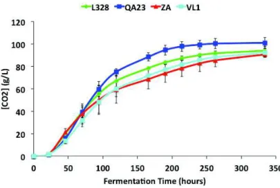
The experiment time was 334 hours in all replicas; the fermentation was considered finish when there was no weight loss between days. With the measure of weight loss it was possible to measure the CO2 production (Figure 4). The results show that the yeast strain QA23 has a

higher production of CO2 during the experience time, an ANOVA shown that the final

concentration is different between strains (p < 0.05). This difference is only mainly because of QA23 high CO2 production. The impact of yeast strain on the exponential phase of the curves

of CO2 release was already reported in the literature [8].

Figure 4.CO2 release during fermentation. Values are the average of three biological repeats ± standard deviation. L328

(cachaça strain), QA23 and VL1 (commercial wine strain) and ZA (laboratory wine strain).

The consumption kinetics (figure 5, A and B) shows that, for all yeast strains, fermentation of fructose always delays when comparing with glucose. This results has been associated with the glucose preference ability of the S. cerevisiae [42]. The fructose kinetics also shows that the selected strains in this work have different preferences regarding fructose, this differences are related to differential rate of nitrogen utilization [43].

36

Figure 5. Fermentation kinetics of the four yeast strains used in this study: glucose (A) and fructose (B) consumption,

ethanol (C) and glycerol (D) formation. All y-axis are in grams per litter and refer to extracellular metabolite concentrations in the synthetic mediums. Values are the average of three biological repeats ± standard deviation.

Although the results showed that ZA, displayed the lowest fructose consumption rate as well as rate of ethanol formation, despite this at the end of alcoholic fermentation no significant differences were observed. However there are significant differences in the glycerol formation, which is reportedly strain dependent [44] [7]. Regarding the ethanol production is known to vary poorly according to the S. cerevisiae strain [45]. The two most important functions of glycerol synthesis in yeast are related to redox balancing and the hyperosmotic stress response. Osmotic stress is one of the most common types of stress imposed on yeasts, making it necessary for the cell to develop mechanisms to survive under these conditions.

A B

37

3.2.

Sensory Analysis

The eleven points of fermentations for each the four strains was evaluated by 20 panellists, males and females, 21 to 50 years of age. The panellists were selected based on their preference for wine, interest and availability. Randomized 10 mL samples of each of the fermentation sampling points were served in black glasses. The panellists were asked whether the aroma of the fermentation products resembled wine or not. Results from the experiments are presented in figure 6.

The highest percentage of panellists describing a “wine-like” aroma was obtained at 142 hours of fermentation (approximately the sixth day). After this the percentage started to decrease because the panellists associate the aroma of the fermentations with the ethanol concentration and not with the “wine-like” feature. In fact some authors reported that ethanol can suppress the perception of several aromas in wines such as fruity notes [46].

Figure 6. Percentage of the panelists that associate the fermentation aroma with the “wine-like” aroma. Values are the

average of three biological repeats ± standard deviation.

The same fermentations samples were also ranked each day from least to most “wine-like”. The transformation of ranks to scores, according Fisher and Yates [47], allowed the quantification of the differences between samples: the lowest the score (more negative) highest the “wine like” aroma of the sample. Results show that L328 and QA23 are the samples that panellists consider more “wine like” and that the VL1 and IVDP are the samples

38 less “wine like”. With the data obtained from the ranking test was subjected to ANOVA to determine whether the panellists could differentiate between yeast strains. The results show that there was no difference in the ranking results of different strains until 142 hours of fermentation and after this time this difference disappear possibly related to the high concentration of ethanol present in the samples. This ethanol effect had already been observed in the first sensorial test for the detection of “wine-like” aroma (Figure 6).

3.3. Volatiles Formation

This study examined the effect of the volatiles compounds on the wine aroma perception. Using a target approached, 26 compounds were analysed during the fermentations of the different strains in all replicates.

Volatile odour/flavour compounds synthesized by yeast strains during fermentation and confirmed by GC-MS were ethyl butanoate, ethyl hexanoate, ethyl heptanoate, ethyl octanoate, ethyl nonanoate, ethyl decanoate, ethyl dodecanoate, hexyl acetate, isoamyl acetate, isoamyl hexanoate, isoamyl octanoate, ethyl phenylacetate, 2-phenylethanol, isovaleric acid, hexanoic acid, octanoic acid and decanoic acid. The compounds confirmed by GC-FID were 1-propanol, 2-methyl-1-propanol, 2-methyl-1-butanol, 3-methyl-1-butanol, acetaldehyde and ethyl acetate. The HPLC measured glycerol, acetic acid and ethanol concentrations.

To the data obtained of compounds concentrations was applied a metabolic synchronization, this means that the original data was divided by the CO2 cumulative

concentration of the same experiment points. This method is crucial because it is aligned with the growth pattern of the organism; the use of synchronized data is more stable and more robust than the original approach based on an imposed time period. The normalization treatment to reduce the time’s influence was proposed to obtain information related to yeast strain differences when using multi-variate analysis [48]. The example (Figure 7) shows the effect of this normalization, in the graphic with the CO2 synchronization we can observe a

39

Figure 7.Ethyl butanoate production rates by concentration of CO2 (A) and by time (B)

3.3.1. Targeted approach

Targeted metabolomics is a quantitative method where a set of known metabolites is quantified. This approach takes advantage of the comprehensive understanding of the fermentation end products and the known biochemical pathways to which they contribute[49]. As a start, a one-way ANOVA (with factor strain type) was performed on the volatiles data set. The quantitative values of the concentrations are represented in the Table 2 for the last point of fermentation and in the Table 3 for the fermentation time of higher “wine-like” (142 hours) as well as the ANOVA results.

A

40

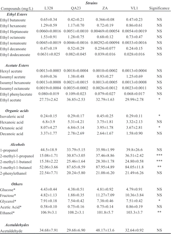
Table 2. Average concentrations of the measured compounds of all replicas ± standard deviation in the last point of fermentation.

Strains

Compounds (mg/L) L328 QA23 ZA VL1 Significance

Ethyl Esters Ethyl butanoate 0.65±0.34 0.42±0.21 0.366±0.08 0.47±0.23 NS Ethyl hexanoate 1.29±0.59 1.17±0.70 0.72±0.19 0.86±0.61 NS Ethyl Heptanoate 0.0060±0.0016 0.0051±0.0010 0.00469±0.00054 0.0054±0.0019 NS Ethyl octanoate 1.53±0.91 1.28±0.75 0.68±0.12 0.73±0.47 NS Ethyl nonanoate 0.0045±0.0019 0.0046±0.0016 0.00292±0.00094 0.0033±0.0016 NS Ethyl decanoate 0.47±0.19 0.52±0.29 0.254±0.077 0.24±0.15 NS Ethyl dodecanoate 0.0631±0.025 0.082±0.045 0.039±0.016 0.028±0.016 NS Acetate Esters Hexyl acetate 0.0013±0.0003 0.0018±0.0004 0.0010±0.0002 0.0013±0.0004 NS Isoamyl acetate 0.69±0.36 1.38±0.48 0.93±0.27 1.25±0.69 NS Isoamyl hexanoate 0.0013±0.0008 0.0021±0.0015 0.0013±0.0005 0.0013±0.0008 NS Isoamyl octanoate 0.0019±0.0004 0.0035±0.0002 0.0026±0.0012 0.0023±0.0011 NS Ethyl phenylacetate 0.080±0.019 0.109±0.023 0.079±0.027 0.068±0.017 NS Ethyl acetate 27.73±2.62 36.85±2.53 32.79±1.63 29.99±2.78 * Organic acids Isovaleric acid 0.24±0.15 0.29±0.17 0.45±0.25 0.29±0.11 * Hexanoic acid 6.8±3.9 5.31±4.21 3.75±1.81 3.32±2.13 NS Octanoic acid 8.07±4.27 6.84±5.14 3.95±1.78 3.67±2.81 * Decanoic acid 3.37±1.77 2.78±2.69 2.64±1.67 1.58±0.90 NS Alcohols 1-propanol 44.5±18.9 33.79±5.15 35.98±1.99 39.8±26.6 NS 2-methyl-1-propanol 15.08±1.71 30.87±3.05 37.46±8.86 36.51±2.42 *** 2-methyl-1-butanol 15.38±2.22 25.46±1.64 28.30±1.78 24.80±0.58 *** 3-methyl-1-butanol 52.06±3.66 87.65±8.59 87.95±4.89 84.05±11.8 ** 2-phenylethanol 22.54±7.71 20.24±5.80 21.08±6.20 21.49±6.26 NS Others Glucose* 4.43±0.44 4.38±0.51 4.81±0.92 4.79±0.91 NS Fructose* 4.82±1.13 1.88±0.35 11.27±7.09 10.36±3.84 NS Glycerol* 7.91±0.18 7.54±0.42 7.38±0.46 7.51±0.42 * Acetic Acid* 0.58±0.10 0.75±0.16 0.75±0.14 0.86±0.19 NS Ethanol* 106.9±3.1 108.2±3.1 101.8±5.7 103.3±3.7 ** Acetaldehydes Acetaldehyde 34.68±7.91 29.68±6.90 48.17±13.6 32.64±0.92 NS

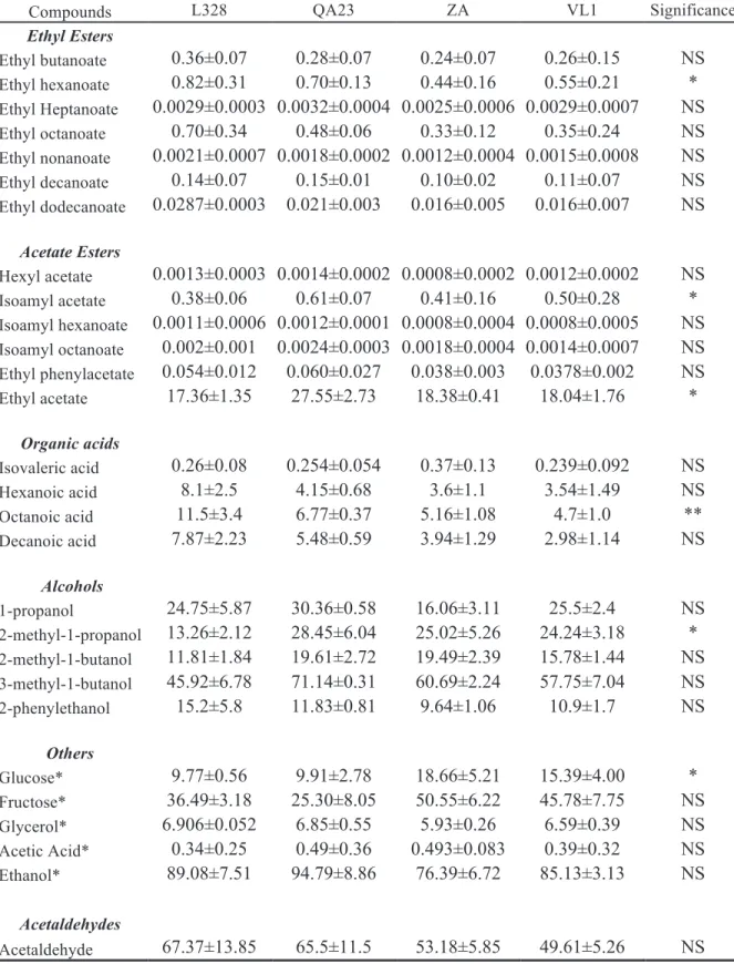
41 Table 3. Average concentrations of the measured compounds of all replicas ± standard deviation in the point of fermentation

with more wine-like (142 hours).

Strains

Compounds L328 QA23 ZA VL1 Significance

Ethyl Esters ! ! ! ! ! Ethyl butanoate 0.36±0.07 0.28±0.07 0.24±0.07 0.26±0.15 NS Ethyl hexanoate 0.82±0.31 0.70±0.13 0.44±0.16 0.55±0.21 * Ethyl Heptanoate 0.0029±0.0003 0.0032±0.0004 0.0025±0.0006 0.0029±0.0007 NS Ethyl octanoate 0.70±0.34 0.48±0.06 0.33±0.12 0.35±0.24 NS Ethyl nonanoate 0.0021±0.0007 0.0018±0.0002 0.0012±0.0004 0.0015±0.0008 NS Ethyl decanoate 0.14±0.07 0.15±0.01 0.10±0.02 0.11±0.07 NS Ethyl dodecanoate 0.0287±0.0003 0.021±0.003 0.016±0.005 0.016±0.007 NS ! Acetate Esters ! ! ! ! ! ! ! ! ! ! Hexyl acetate 0.0013±0.0003 0.0014±0.0002 0.0008±0.0002 0.0012±0.0002 NS Isoamyl acetate 0.38±0.06 0.61±0.07 0.41±0.16 0.50±0.28 * Isoamyl hexanoate 0.0011±0.0006 0.0012±0.0001 0.0008±0.0004 0.0008±0.0005 NS Isoamyl octanoate 0.002±0.001 0.0024±0.0003 0.0018±0.0004 0.0014±0.0007 NS Ethyl phenylacetate 0.054±0.012 0.060±0.027 0.038±0.003 0.0378±0.002 NS Ethyl acetate 17.36±1.35 27.55±2.73 18.38±0.41 18.04±1.76 * ! _{Organic acids} ! ! ! ! ! ! ! ! ! ! Isovaleric acid 0.26±0.08 0.254±0.054 0.37±0.13 0.239±0.092 NS Hexanoic acid 8.1±2.5 4.15±0.68 3.6±1.1 3.54±1.49 NS Octanoic acid 11.5±3.4 6.77±0.37 5.16±1.08 4.7±1.0 ** Decanoic acid 7.87±2.23 5.48±0.59 3.94±1.29 2.98±1.14 NS ! Alcohols ! ! ! ! ! ! ! ! ! ! 1-propanol 24.75±5.87 30.36±0.58 16.06±3.11 25.5±2.4 NS 2-methyl-1-propanol 13.26±2.12 28.45±6.04 25.02±5.26 24.24±3.18 * 2-methyl-1-butanol 11.81±1.84 19.61±2.72 19.49±2.39 15.78±1.44 NS 3-methyl-1-butanol 45.92±6.78 71.14±0.31 60.69±2.24 57.75±7.04 NS 2-phenylethanol 15.2±5.8 11.83±0.81 9.64±1.06 10.9±1.7 NS ! Others ! ! ! ! ! ! ! ! ! ! Glucose* 9.77±0.56 9.91±2.78 18.66±5.21 15.39±4.00 * Fructose* 36.49±3.18 25.30±8.05 50.55±6.22 45.78±7.75 NS Glycerol* 6.906±0.052 6.85±0.55 5.93±0.26 6.59±0.39 NS Acetic Acid* 0.34±0.25 0.49±0.36 0.493±0.083 0.39±0.32 NS Ethanol* 89.08±7.51 94.79±8.86 76.39±6.72 85.13±3.13 NS Acetaldehydes Acetaldehyde 67.37±13.85 65.5±11.5 53.18±5.85 49.61±5.26 NS

42 3.4.2.3. Unsupervised Techniques

The goal for the use of SVD was to examine the intrinsic variation in the data set, in order to determine if the selected target compounds are capable to discriminate fermentations performed by different strains. Because the aim of this study is to identify the metabolites that are important for the “wine-like” sensory feature, the two data sets were fused into one overall metabolomics set. This resulted in a data matrix consisting of 148 samples and 27 variables. Was applied a Singular Value Decomposition (SVD) to the normalized data of the concentrations together with the data from the sensorial analysis (the responses to a positive detection of “wine-like” aroma). This study is sensory driven so we sought to identify the compounds that are correlated with the “wine-like” aroma. This technique helps to understand the volatile composition and their association with the “wine-like” feature felt by the consumers.

Using PCA, the chemical and sensory data obtained were modelled. The root mean square error of cross validation (RMECV), takes minimum values at 4 principal components. PCA shows plot that 97% of variation is explained by the first four principal components, and that replicate fermentation measurements group together.

The sensorial data, relating to the “wine-like” aroma, was appended to the normalized data of the target compounds. This study is sensory driven, so we sought to identify the compounds that are correlated with the “wine-like” aroma. The score plots for the first three components were projected against time of fermentation in hours and the cumulative CO2 release (figure

8).

The first two principal components (PC1 and PC2 in figure 9) explained 46.28% and 18.01% of the total variance. In the biplot, PC1 is represented the evolution of the fermentation, this means the formation of compounds, the effect is not very marked because of the normalization by the CO2 which decrease the time impact.

The second component explained the variance obtained with the sensorial results. In the positive side of PC2 we observe the loading (purple dots) of “wine-like” feature together with acetaldehyde, hexyl acetate and ethyl esters. These compounds are in an orthogonal position with the higher alcohols and acetate esters. The good correlation of acetaldehyde with “wine-like” aroma as already been commented in the literature [50], it is reported that acetaldehyde give a desirable aroma to wines. Ethyl esters were also described as fruity and wine-like [4]

43 while higher alcohols are described as harsh and unpleasant [6]. In this analysis no strain could be differentiated, indicating that regarding the “wine-like” aroma there no big differences between strains.

Figure 8.Principal component analysis score plot of PC1, PC2 and PC3 projected against fermentation time (A) and CO2

44

Figure 9. Singular value decomposition plot: PC1 vs. PC2 and PC1 vs. PC3 of the normalized volatile data obtained

combined with the “wine-like”

When plotting PC1 with PC3 (figure 9) we can observe that the L328 (red marks) strain highly differentiated from the others strains mainly because of the production of ethyl esters as we can see in the loadings (purple dots). On the extremes of PC3 we can observe the higher alcohols and acetates in the positive side and the ethyl esters in the negative side. This means that when were produced more ethyl esters also were produced less higher alcohols. As we can see in Figure 11, L328 strain (red marks) has low concentration in 2 methyl-1-propanol

PC 1 (45.24%) -0.2 -0.15 -0.1 -0.05 0 0.05 0.1 0.15 0.2 PC 2 (18.30%) -0.1 -0.05 0 0.05 0.1 0.15 C4C2 C6C2 C7C2 C8C2 C10C2 Hexyl acetate IsoAcetate HexaAcetate EtPhAcetate iC5 C6 C8 Acetaldehyde EtAcetate 1-prop 2met1prop 2met1but 3met1but Gly Acetic Acid Ethanol Winelike Biplot of data Class 0 L328 QA23 VL1 ZA Class 0 (Selected) PC 1 (45.24%) -0.15 -0.1 -0.05 0 0.05 0.1 0.15 PC 3 (13.08%) -0.1 -0.08 -0.06 -0.04 -0.02 0 0.02 0.04 0.06 0.08 C4C2 C6C2 C8C2 C9C2 C10C2 C12C2 Hexyl acetate IsoAcetate HexaAcetate OctaAcetate Phenylol EtPhAcetate iC5 C6 C8 C10 Acetaldehyde EtAcetate 1-prop 2met1prop _2met1but 3met1but Gly Acetic Acid Ethanol Winelike Biplot of data Class 0 L328 QA23 VL1 ZA Class 0 (Selected) Decluttered

45 (higher alcohol) but higher concentration in ethyl octanoate (ethyl ester). The fact that ester composition of wines is strain dependent has been reported [51] [52].

This behave was described on a metabolic way in the literature. Differences in regulation of the synthesis of ethyl esters are due to the fatty acid metabolism being the main factor influencing it, whereas the production of higher alcohols and acetates is influenced by the Ehrlich pathway and the presence of alcohol acetyltransferases [53].

All this knowledge can be quite useful for wine industry since it allows the possibility of modifying wine aroma by either increasing the desirable or eliminating the undesirable compounds.

Projection of PC1 vs. PC4 (5.11% variance) shows a separation between replicas. The results (Figure 10) show that replica 3 (blue marks) is highly differentiated from the others replicas, the principal factor of this difference is the production of acetic acid. This difference is not very representative because only explain 5.11% of variance in the data so the spoilage of this replica by an acectobater. Acetic acid formation by strains of S. cerevisiae is affected by sugar concentration, pH and nitrogen [54] so a small difference in the medium preparation or ambient conditions can be cause of this separation. Since the PC1 refers to fermentation evolution we can clearly see that the second replica (green dots) had lower concentrations of the volatiles compounds.

Figure 10. Principal component analysis: PC1 vs PC4 of the normalized volatile data obtained combined with the

“wine-like” feature. PC 1 (45.24%) -0.15 -0.1 -0.05 0 0.05 0.1 0.15 PC 4 (5.57%) -0.08 -0.06 -0.04 -0.02 0 0.02 0.04 0.06 C4C2 C6C2 C7C2 C8C2 C9C2 C10C2 C12C2 HexaAcetate OctaAcetate Phenylol EtPhAcetate iC5 C6 C8 Acetaldehyde EtAcetate 1-prop 2met1prop 2met1but 3met1but Gly Acetic Acid Ethanol Winelike Biplot of data Class 0 R1 R2 R3 Class 0 (Selected)

Decluttered Class Set: Replicas

46 Cluster analysis technique generates a category structure, which fits a set of observations. The groups that are formed have a high degree of association between members.

Unsupervised two-way agglomerative hierarchical cluster analysis (HCA) assessed the similarities between individual metabolome profiles. This algorithm used a multivariate Euclidean distance metric and Ward’s group linkage. The results were displayed as a heat map (green=low metabolite concentration, red = high metabolite concentration) with associated cluster dendrograms; the lower the linkage distances in the dendrogram the more similar the feature. Metabolites that were most similar across all samples, and samples that were most similar across all metabolites, form the lowest linkage in the respective dendrograms. Prior to PCA and HCA each metabolite feature was scaled to unit variance (auto scaled), which allows each metabolite to be compared within the analysis with no bias due to differences in absolute concentration variance

The results (Figure 11) show the same conclusions of the SVD, when we can clearly see the two different groups. Compounds that are mainly from Fatty acid metabolism and compound that have connections with the Ehrlich Pathway, being the “wine-like” feature connected with the compounds of the first group (mainly ethyl esters). The results also show that the strain L328 has a good correlation the “wine-like” effect; hence it has a good correlation with ethyl esters and a low correlation with the higher alcohols as expected.

47

Figure 11. Cluster analysis of the fermentations data combined with “wine-like” feature.

The compounds used in this analysis were ethyl butanoate (C4C2), ethyl hexanoate (C6C2), ethyl heptanoate (C7C2), ethyl octanoate (C8C2), ethyl nonanoate (C9C2), ethyl decanoate (C10C2), ethyl dodecanoate (C12C2), hexyl acetate, isoamyl acetate, isoamyl hexanoate, isoamyl octanoate, ethyl phenylacetate, 2-phenylethanol, isovaleric acid (iC5), hexanoic acid (C6), octanoic acid (C8), decanoic acid (C10), 1-propanol, propanol, 2-methyl-1-butanol, 3-methyl-1-2-methyl-1-butanol, acetaldehyde, ethyl acetate, glycerol, acetic acid and ethanol.

48 3.4.2.3. Supervised Techniques

PLS-regression analysis (PLS-R) is a linear regression model by projecting the category and the observable variables onto a new space by maximizing the correlation between two data sets.

In this study PLS-R is used to find the relations between the metabolite data and the selected sensory attribute (figure 12). Table 4 shows the model performance. For “wine-like” sensory feature very important projection (VIP’s) leads to 9 metabolites.

With the data obtained with the targeted approach (the quantification of compounds) was applied a PLS to try get a prediction model by using the concentrations to get “wine-like” feature.

Several compounds play a key role in wine aroma, which is very important for the consumer buying decision. So the acceptance of the “wine-like” aroma needs to be measured during wine production. The traditional sensory analysis is the preferred method for evaluation of odor, but are expensive to implement, time consuming and cannot be implemented “on-line” for immediate feedback [55].

Figure 12. PLS-R method for “wine-like” feature for prediction in fermentation

Y Measured 1 0 0.5 1 1.5 2 2.5 3 3.5 4 4.5 5 Y CV Predicted 1 -0.5 0 0.5 1 1.5 2 2.5 3 3.5 4

4.5 Samples/Scores Plot of data

CV Bias = -0.0113 R2 _{= 0.805}

3 Latent Variables Calibration Bias = 8.8818e-16 RMSEC = 0.35893 RMSECV = 0.4038 Wine-like measured W in e -l ik e p re d ic te d

49 Figure 14 shows the predicted “wine-like” values (percentage of recognition) compared with the measured values in sensory analysis. The calibration model for “wine-like” feature performed well, with a coefficient of determination (R2) of 80.5%. The validation statistics of the performance of the calibration are shown in Table 5. The low differences attained between RMSEC (0.35893) and RMSECV (0.4038) values show that the built models are near to the real situations of the samples set [56]. The number of latent variables for this calibration model was 3.

Table 4. Validation statistics of the performance of PLS method on prediction of "wine-like" feature.

CV Bias -0.0113

R2 0.805

Latent Variables 3

Calibration Bias 8.88e-16

RMSEC 0.35893

RMSECV 0.4038

Figure 13 summarizes the influential volatile compounds in the construction of the model. Variable Importance in Projection (VIP) scores estimate the importance of each variable in the projection used in a PLS model and is often used for variable selection. A variable with a VIP Score close to or greater than 1 (one) can be considered important in given model. Variables with VIP scores significantly less than 1 (one) are less important and might be good candidates for exclusion from the model.

50

Figure 13. Distribution of volatiles compounds in accordance with PLS model

The most important compounds (higher than one) for the prediction of “wine-like” feature were acetaldehyde, hexyl acetate and glycerol. These same compounds were already commented as well correlated with the sensorial feature in the SVD method showing big impact on the aroma. The compounds ethyl butanoate, ethyl hexanoate, hexanoic acid and octanoic acid also have an impact in the construction of the model.

Variable

0 5 10 15 20 25 30

VIP Scores for Y 1

0 0.5 1 1.5 2 2.5 3 3.5 4 4.5 C4C2 C6C2 C7C2 C8C2 C9C2 C10C2 C12C2 Hexyl acetate IsoAcetate HexaAcetate OctaAcetate Phenylol EtPhAcetate iC5 C6 C8 C10 Acetaldehyde EtAcetate 1-prop 2met1prop 2met1but 3met1but Gly Acetic Acid Ethanol

Variables/Loadings Plot for data

Figure 14.PLS-R method for “wine-like” feature for prediction in fermentation before 142 hours (maximum wine-like)

W in e -l ik e p re d ic te d Wine-like measured