Influence of the molecular weight in mechanical properties and degradation kinetics of chitosan inverted colloidal crystals

(1)

Setembro, 2014

Ana Teresa Guerra Kullberg

[Nome completo do autor]

Licenciatura em Ciências de Engenharia de Materiais

[Habilitações Académicas]

Influence of the molecular weight on the mechanical

properties and degradation kinetics of chitosan inverted

colloidal crystals

[Título da Tese]

Dissertação para obtenção do Grau de Mestre em

Engenharia de Materiais

Dissertação para obtenção do Grau de Mestre em

[Engenharia Informática]

Orientador:

Prof. Doutor João Paulo Miranda Borges, Professor Auxiliar, FCT-UNL

Co-orientadores: Prof. Doutor Jorge Alexandre Monteiro Carvalho Silva, Professor

Auxiliar, FCT-UNL

Mestre Carlos Filipe Cidre João, FCT-UNL

Júri:

Presidente: Prof. Doutor João Pedro Botelho Veiga

Arguente: Prof. Doutora Ana Isabel Nobre Martins Aguiar de Oliveira Ricardo Vogal: Prof. Doutor João Paulo Miranda Ribeiro Borges

(2)

(3)

iii

Influence of the molecular weight in mechanical properties and degradation kinetics of chitosan inverted colloidal crystals

A Faculdade de Ciências e Tecnologia e a Universidade Nova de Lisboa têm o direito, perpétuo e sem limites geográficos, de arquivar e publicar esta dissertação através de exemplares impressos reproduzidos em papel ou de forma digital, ou por qualquer outro meio conhecido ou que venha a ser inventado, e de a divulgar através de repositórios científicos e de admitir a sua cópia e distribuição com objectivos educacionais ou de investigação, não comerciais, desde que seja dado crédito ao autor e editor.

(4)

(5)

v

Agradecimentos

Aos meus orientadores, Professor Doutor João Paulo Borges, Professor Doutor Jorge Carvalho Silva e Mestre Carlos João, pelo entusiasmo, disponibilidade e dedicação demonstrados no decorrer do trabalho, bem como pela partilha de conhecimentos.

À Pontes, por todos os momentos partilhados, dentro e fora da faculdade, que tornaram estes últimos tempos muito mais fáceis. Pela ajuda que nunca me negou, por toda a força e incentivo, mesmo nos momentos menos bons. Acima de tudo, por acreditar sempre em mim, mesmo quando eu própria duvidei. Não imaginas o quanto te admiro.

Alex, por tantas horas partilhadas e pelas conversas profundas e filosóficas sobre utopias. Ao Marreiros, que sempre esteve presente quando precisei, pela companhia e apoio.

À Rute, por todas as horas e trabalho partilhado, mas principalmente por me ter substituído nas alturas em que mais precisei.

À Joana, pela constante alegria, que fez com que mesmo nos momentos mais complicados houvesse sempre motivo para rir.

Ao Anselmo, pela boa disposição constante.

À Susana, pelo adorável mau feitio, a quem tenho que deixar também uma palavra de incentivo para o que aí vem.

Ao Chico, pela companhia e gargalhadas contagiantes. Ao Zé Rui, pelo otimismo e aleatoriedade.

Ao Gui, por toda a amizade e por sempre me ter apoiado incondicionalmente em todas as situações. Certamente uma das pessoas mais incríveis que conheço.

Aos meus amigos de sempre: a Bárbara, a Joana, a Loira, o Tiago e o Alex, por serem as excelentes pessoas que são, por todos os momentos partilhados e por mostrarem como é possível manter uma amizade sólida, independentemente dos caminhos seguidos.

A todo o grupo de Soft and Biofunctional Materials do DCM, em particular à Paula Soares e à Coro, por toda a disponibilidade, incentivo e pelas palavras experientes que foram tão importantes para superar este desafio.

À Andreia Lopes, do grupo de Materiais Estruturais, pela disponibilidade e simpatia que sempre demonstrou.

À minha família, em particular ao meu Mano, por toda a cumplicidade e proteção.

Por fim, e acima de tudo, devo um agradecimento muito especial aos meus Pais, pela educação e valores que me transmitiram, pelos sacrifícios feitos ao longo deste percurso, pela compreensão e apoio incondicional, essenciais em particular nesta última etapa.

(6)

(7)

vii

Abstract

Tissue engineering arises from the need to regenerate organs and tissues, requiring the development of scaffolds, which can provide an optimum environment for tissue growth.

In this work, chitosan with different molecular weights was used to develop biodegradable 3D inverted colloidal crystals (ICC) structures for bone regeneration, exhibiting uniform pore size and interconnected network. Moreover, in vitro tests were conducted by studying the influence of the molecular weight in the degradation kinetics and mechanical properties.

The production of ICC included four major stages: fabrication of microspheres; assembly into a cohesive structure, polymeric solution infiltration and microsphere removal.

Chitosan’s degree of deacetylation was determined by infrared spectroscopy and molecular weight was obtained via capillary viscometry. In order to understand the effect of the molecular weight in ICC structures, the mass loss and mechanical properties were analyzed after degradation with lysozyme. Structure morphology observation before and after degradation was performed by scanning electron microscopy. Cellular adhesion and proliferation tests were carried out to evaluate ICC in vitro response.

Overall, medium molecular weight ICC revealed the best balance in terms of mechanical properties, degradation rate, morphology and biological behaviour.

Keywords: Inverted colloidal crystals, Bone tissue engineering, Chitosan, Molecular weight,

(8)

(9)

ix

Resumo

A engenharia de tecidos advém da necessidade de regenerar órgãos e tecidos, requerendo o desenvolvimento de matrizes porosas que ofereçam um ambiente ideal para o desenvolvimento de tecido.

Neste trabalho, utilizou-se quitosano com diferentes pesos moleculares para a produção de estruturas 3D biodegradáveis para a regeneração de tecido ósseo, com a geometria de réplicas invertidas de cristais coloidais (ICC). Foram também realizados testes in vitro, através do estudo da influência do peso molecular na cinética de degradação e nas propriedades mecânicas.

A produção de ICC inclui essencialmente quatro etapas: produção de microesferas, construção de uma estrutura coesa, infiltração com uma solução polimérica e remoção das microesferas.

O grau de desacetilação do quitosano foi determinado por espectroscopia de infravermelho e o peso molecular foi obtido por viscosimetria capilar. De forma a compreender o efeito do peso molecular na estrutura dos ICC, a perda de massa e as propriedades mecânicas foram analisadas após a degradação com lisozima. A observação da morfologia da estrutura, antes e depois da degradação, foi realizada através de microscopia eletrónica de varrimento. Testes de adesão e proliferação celular foram efetuados, para avaliar o comportamento in vitro dos ICC.

De um modo geral, os ICC produzidos com peso molecular médio revelaram o melhor equilíbrio ente propriedades mecânicas, taxa de degradação, morfologia e comportamento biológico.

Palavras-chave: Réplicas invertidas de cristais coloidais, Engenharia de tecido ósseo, Quitosano, Peso

(10)

(11)

xi

List of Figures

Figure 2.1 -Structural organization of the human bone [6]... 3 Figure 2.2 - SEM images of (a) high periodicity colloidal crystals and (b) its respective inverted colloidal crystals, produced with polyacrylamide (adapted from [15]). ... 5

Figure 2.3 – Chemical structure of partially acetylated chitosan, a copolymer characterized by its average degree of deacetylation (1-DA), composed by (a) N-acetyl-glucosamine and (b) N-glucosamine units. ... 6

Figure 3.1 – Schematic representation of the microfluidics setup assembled. ... 10 Figure 3.2 – Schematic representation of the mould used in the production of colloidal crystals (a) with the different layers apart and (b) after assembly, ready to use; each well has a diameter of 5.93 mm and is 4.00 mm height. ... 10

Figure 3.3 – Schematic representation of the 24 well plate used in this experiment, with the wells identified according to their content (LCe – LMw ICC with cells; LMC – LMw ICC without cells (control); MCe – MMw ICC With cells; MMC – MMw ICC control; HCe – HMw ICC with cells; HMC – HMw ICC control; CeC – Cell control; MC – Medium control). ... 13

Figure 4.1 – Effect of the amount of NaNO2 on the Mw of chitosan. ... 15 Figure 4.2 – POM image of a PS microsphere, obtained by microfluidics, in which it is possible to observe the characteristic uniform shape. ... 16

Figure 4.3– SEM images of (a) a CC annealed at 120C and (b) the respective inverse replica. ... 17 Figure 4.4 – SEM images of a CC annealed at 130C, with different ampliations. ... 17 Figure 4.5 – SEM images of (a) ICC with 2% CS, (b) ICC with 3% CS and (c) ICC with 4% CS. ... 18 Figure 4.6 – Infrared spectra of different molecular weight CS. ... 19 Figure 4.7 - Mass loss evolution throughout the degradation time, for () HMw, (▲) MMw and (■) LMw CS. ... 20

Figure 4.8 – Compression moduli evolution throughout the degradation time, for () HMw, (▲) MMw and (■) LMw CS. ... 21

Figure 4.9 - Compression modulus evolution with the molecular weight of the chitosan, in (■) freeze-dried scaffolds and in () ICC. ... 22

Figure 4.10 – SEM image of a non-degraded high molecular weight CS ICC. ... 23 Figure 4.11 – SEM images of high molecular weight samples with (a) one, (b) two, (c) three and (d) four weeks degradation. ... 24

Figure 4.12 - SEM image of a non-degraded medium molecular weight CS ICC. ... 25 Figure 4.13 – SEM images of medium molecular weight samples with (a) one, (b) two, (c) three and (d) four weeks degradation. ... 25

Figure 4.14 - SEM image of a non-degraded low molecular weight CS ICC. ... 26 Figure 4.15 – SEM images of low molecular weight samples with (a) two, (b) three and (c,d) four weeks degradation. ... 26

(14)

xiv

Figure 4.16 – Absorbance evolution throughout SaOs-2 culture time, for H0, M0 and L0 ICC. . 28

Figure 4.17 – MO images of different regions of a HMw ICC, exhibiting some cell agglomerates (bright dots). ... 29

Figure 4.18 - MO images of the same area of a MMw ICC, with different focus ranges, exhibiting cell agglomerates all over the structure. ... 29

Figure 4.19 - MO images of the same area of a LMw ICC, with different focus ranges, showing no visible cells. ... 30

Figure 4.20 - SEM images of different areas of a MMw ICC, exhibiting a cell layer all over the structure. ... 30

Figure 6.1– Schematic representation of the Ubbelohde glass capillary used in this work. ... 37

Figure 6.2 – Plot of the reduced viscosity as a function of the concentration (example). ... 38

Figure 6.3 - Plot of the inherent viscosity as a function of the concentration (example). ... 39

Figure 6.4 – Example of an ICC’s stress-strain curve obtained during compression tests. ... 40

Figure 6.5– Compression modulus evolution throughout the degradation time, for high molecular weight CS. ... 41

Figure 6.6– Compression modulus evolution throughout the degradation time, for medium molecular weight CS. ... 41

Figure 6.7– Compression modulus evolution throughout the degradation time, for low molecular weight CS. ... 42

(15)

xv

List of Tables

Table 3.1– Chitosan solutions used for viscometry. ... 11

Table 4.1 – Chitosan molecular weight values obtained for each NaNO2 mass used in the reaction; each value represents an average of three measurements. ... 15

Table 4.2 – Mass concentrations used in the production of CS solutions, for each molecular weight. ... 18

Table 4.3 – Degrees of deacetylation obtained for each molecular weight. ... 20

Table 4.4 – Cell adhesion after 24h, for different molecular weight ICC. ... 28

Table 6.1– Parameters of the viscometry essays and constants for the used solvent. ... 37

Table 6.2 – Mass loss percentage per degradation set; each set is composed by 10 ICC. ... 39

Table 6.3 – Average mechanical properties obtained for each degradation sample and the respective relative standard deviation; each value was obtained with sets of approximately 10 ICC. . 40

Table 6.4 – Mechanical properties of the freeze-dried scaffolds and ICC, according to the different molecular weights. ... 42

Table 6.5. – Mechanical properties of the human bone [44]. ... 42

Table 6.6 – Porosity values obtained for each ICC set, according to the Ashby and Gibson model for cellular solids. ... 43

(16)

(17)

xvii

Symbology

A1655 Absorbance at 1655 cm-1 A3450 Absorbance at 3450 cm-1

md Dry-state mass

tsolvent Efflux time for the solvent E Elastic Modulus of a scaffold Es Elastic Modulus of a solid

mh Hydrated mass

ηinh Inherent Viscosity [η] Intrinsic Viscosity

w/w Mass Fraction

P Porosity

ηred Reduced Viscosity

ηr Relative Viscosity  Scaffold density s Solid density ηsp Specific Viscosity ms Submerged mass η Viscosity v/v Volume Fraction

(18)

(19)

xix

Abbreviations

ATR Attenuated Total Reflectance

CC Colloidal Crystals

CeC Cell control

CS Chitosan

DA Degree of acetylation

DAPI Fluorescent Nucleic Acid

DD Degree of deacetylation

FCC Face-Centered Cubic

FTIR Fourier Transform Infrared Spectroscopy H0 Non-degraded high molecular weight H1 High molecular weight (1 week degradation) H2 High molecular weight (2 weeks degradation) H3 High molecular weight (3 weeks degradation) H4 High molecular weight (4 weeks degradation)

HCe HMw ICC with cells

HEW Hen Egg White

HCP Hexagonal Close-Packed

HMC HMw ICC control

HMw High Molecular Weight

ICC Inverted Colloidal Crystals

L0 Non-degraded low molecular weight L1 Low molecular weight (1 week degradation) L2 Low molecular weight (2 weeks degradation) L3 Low molecular weight (3 weeks degradation) L4 Low molecular weight (4 weeks degradation)

LCe LMw ICC with cells

LMC LMw ICC without cells (control)

LMw Low Molecular Weight

M0 Non-degraded medium molecular weight M1 Medium molecular weight (1 week degradation) M2 Medium molecular weight (2 weeks degradation) M3 Medium molecular weight (3 weeks degradation) M4 Medium molecular weight (4 weeks degradation)

MC Medium control

MCe MMw ICC with cells

MHS Mark-Houwink-Sakurada

MMC MMw ICC control

MMw Medium Molecular Weight

(20)

xx

OM Optical Microscope

PBS Phosphate Buffered Saline POM Polarized Optical Microscope

PS Polystyrene

PVA Poly(vinyl alcohol) SaOs-2 Sarcoma Osteogenic

SEM Scanning Electron Microscopy T25 Tissue culture flask (25 cm2₎

(21)

1

1. Motivation and objectives

Tissue engineering employs the principles of engineering and life sciences to develop biological substitutes that replace, regenerate or improve the function of injured tissues [1,2]. The structure and properties of the scaffolds used in tissue engineering have been extensively studied.

Numerous results show that a scaffold with a 3D structure interconnected by a network of channels is extremely important for a successful tissue regeneration [3]. Pore size and interconnectivity play a vital role in cell culture, being responsible for the adhesion, migration and exchange of nutrients and metabolite wastes. Several production methods were proposed in order to create scaffolds which can provide an ideal environment, but they all seem to be rather limited in terms of capability and feasibility, typically leading to structures with irregular pore size and shape, as well as poor interconnectivity [1].

Inverted colloidal crystals have recently become object of study in tissue engineering. These scaffolds possess uniform pore size, shape, distribution and interconnectivity. Chitosan ICC combine the structure’s unique properties, in terms of morphology, with biocompatibility and biodegradability. Additionally, these scaffolds can exhibit nanofibrous texture on the wall surface, which led several groups to consider it an ideal system for tissue engineering [4,5].

Degradation kinetics is one of the most important issues when developing biological substitutes. Furthermore, mechanical properties have to be taken into account, in order to best suit the injured tissue. For these reasons, the main purpose of this work was to study the influence of the molecular weight of chitosan in the degradation kinetics and mechanical properties of inverted colloidal crystals.

(22)

(23)

3

2. Introduction

2.1. Bone Tissue

Bone is an extremely organized and specialized connective tissue [6]. This tissue has a complex hierarchical structure, meaning that it has distinct structural arrangements in different scales, extending from the nano to the macroscopic level [7].

Macroscopically, bone tissue has two different architectures: cortical, or compact, and cancellous, or trabecular. The first type has a higher density and constitutes the external layer of the bone, having higher Young Modulus. In contrast, trabecular bone is a porous material [6]. Such combination enables a balance between stiffness and ductility. Microscopically (10-500 m), it is possible to identify Haversian systems, osteons and single trabeculae. The sub-microstructure (1-10 m) consists of lamellae. At the nanoscale (100 nm–1 m), one can distinguish collagens fibrils and apatite crystals. Finally, the subnanostructure is composed by the molecular structure of constituent elements, such as mineral, collagen and other organic proteins [6,7]. This kind of architecture, which can be observed in Figure 2.1, provides a combination of outstanding mechanical properties (see Table 6.5, appendix – section 6.3) and biological response, allowing the bone to perform distinct functions, from structural support to cell protection and storage [6-8].

Figure 2.1 -Structural organization of the human bone [6].

In terms of composition, bones are natural composites, in which about 65% consists of an inorganic phase (carbonate hydroxyapatite) and the remaining is composed by organic matter (mostly collagen) and water [9].

(24)

4

2.2. Scaffolds

Frequently, bone lesions heal well under standard therapy, but when bone fractures or defects are larger than a critical-size, they cannot regenerate exclusively through normal physiological processes, requiring bone grafting [2]. Bone grafts are usually autologous (from the patient’s own body), but can also be allograft (cadaveric bone), xenograft (different species) or synthetic (scaffolds) [10]. These last can be polymeric, ceramic or composites, normally consisting of a ceramic (usually calcium phosphates) reinforced polymeric matrix.

Facing a complex and sensitive system as the human body, the requirements of scaffold materials for tissue engineering are particularly challenging [11]. Several experimental results show that it is extremely important for cell seeding, tissue growth and regeneration to have a three-dimensional structure, rather than a bi-dimensional one [4]. Traditional bi-dimensional structures proved to be unable to mimic the environment provided by the original tissue [3].

Generally, there are four main requirements for a scaffold [1,12]:

 The material used must be biocompatible, biodegradable and capable of promoting cell adhesion and migration;

 The scaffold must have a 3D network of interconnected and appropriately sized pores;  The mechanical properties should suit the application and tissue to replace, whether it is bone tissue, blood vessels, cartilage, or any other, in order to temporarily offer structural support until new tissue has formed;

 The degradation rate should match the tissue regeneration rate, so that it provides structural support at first, being reabsorbed once new tissue grows;

Achieving the requirements listed above depends not only on the material used, but also on the production method [4]. Several production techniques, such as electrospinning, phase separation, gas foaming, emulsion freeze drying, high pressure processing, internal bubbling process and particulate leaching, have been widely studied [1,13,14]. However, it was found that all of these methods are limited in at least one specification. Most of these techniques lead to scaffolds with irregularly sized, shaped and dispersed pores. Poor interconnectivity between pores and lack of mechanical strength are also pointed out as recurring problems. These parameters play a crucial role in cell seeding and, consequently, in successfully regenerating an injured tissue. A scaffold with opened, interconnected and organized pores allows an adequate exchange of nutrients, cell movement, penetration and adhesion, as well as in vivo vascularization [1,12]. Therefore, it is vital to use a highly organized structure.

2.2.1. ICC – Inverted Colloidal Crystals

Colloidal crystals are networks of spherical particles with uniform size and shape, arranged in a hexagonal lattice. The diameters of the spheres can reach from nanometers to micrometers, depending on the desired application [4].

Colloidal crystals can be assembled to serve as templates, whose voids can be filled with a variety of solutions. After the material solidifies, the CC particles can be removed, leaving a long-ranged periodic porous structure, composed by the infiltrated material, an ICC. As a result of the Hexagonal

(25)

5

Close Packed (HCP) structure of the CC, each cavity is connected with up to 12 other cavities in an ICC, allowing efficient cell migration and nutrients and oxygen diffusion in all directions [12].

The high periodicity of the networks obtained by aggregating microspheres in colloidal crystals is clearly revealed in Figure 2.2 (a). The respective inverse replicas are shown in Figure 2.2 (b).

Figure 2.2 - SEM images of (a) high periodicity colloidal crystals and (b) its respective inverted colloidal crystals, produced with polyacrylamide (adapted from [15]).

An exceptional uniformity in size, shape and pore distribution, combined with an enhanced interconnectivity, make these matrices an ideal system for tissue engineering. Combining these properties with a biocompatible and bioactive material, one can obtain an excellent environment for cell seeding and tissue regeneration [1,4].

Generally, the production of ICC consists of three major steps [12]:  Fabrication of uniform microspheres;

 Assembly of the microspheres into a HCP lattice;  Production of an inverse replica.

Microspheres can be obtained by microfluidics, a simple method to synthesize monodisperse microparticles. The particle size can easily be controlled by the variation of the flow rates and concentrations of two immiscible fluids [12,16].

The assembly step takes advantage of the fact that microspheres tend to organize into thermodynamically more stable forms, like HCP and Face Centered Cubic (FCC) structures. After the assembly, it is necessary to use a heat treatment (annealing), to create bridges between consecutive microspheres, turning the assembled microspheres into a linked solid structure [12].

The size of the microspheres used determines the structure’s porosity. The size of the “windows” between pores, which defines their interconnectivity, can be controlled during the annealing of the CC, by adjusting time or temperature. Therefore, the morphology of an ICC can easily be adapted to the type of cells which are intended to seed. For bone tissue regeneration, the recommended pore size is between 100 m and 400 m [1].

(26)

6

2.3. Chitosan

Chitin is a copolymer composed by N-acetyl-glucosamine and N-glucosamine units randomly or block distributed, depending on the processing method [13]. When the number of N-glucosamine units (see Figure 2.3) is dominant, meaning that the degree of deacetylation is higher than about 60%, this copolymer is named chitosan [17].

Figure 2.3 – Chemical structure of partially acetylated chitosan, a copolymer characterized by its average degree of deacetylation (1-DA), composed by (a) N-acetyl-glucosamine and (b) N-glucosamine

units.

Concerning its structure, chitosan is considered to be a semi crystalline linear polysaccharide, with repeat units connected by β-(1 → 4) glycosidic linkages [17-19].

Chitosan possesses several features that make it very attractive for a variety of applications, from agriculture, to water treatment and also for the cosmetic industry. However, the most promising uses of this deacetylated derivative of chitin seem to lie in the biomedical, biotechonological and pharmaceutical fields. Its biodegradability, natural origin and low toxicity make it ideal to use in tissue regeneration (in the form of three-dimensional porous scaffolds), as antimicrobial and antifungal agents, as wound dressing and as drug delivery vehicles [19]. Chitosan is often used in bone tissue regeneration in the form of three-dimensional porous scaffolds. Being a naturally occurring polymer, chitosan minimizes foreign-body response, one of the major problems associated with other bone grafts [10].

Additionally, chitosan has a hydrophilic surface that promotes adhesion and proliferation of bone forming cells (osteoblasts) as well as the formation of a mineralized bone matrix in vivo. Several results showed in vivo ossification and osteoinduction, promoted by chitosan. Along with hydroxyapatite, chitosan is one of the few materials classified as bioactive, biodegradable and osteoconductive, placing it among the most promising materials for bone tissue engineering [20].

2.3.1. Molecular Weight

In order to obtain distinct properties, chitosan with different molecular weights can be used. This parameter affects properties like the crystallinity degree, Young modulus and biodegradability. The high viscosity inherent to high molecular weight chitosan solutions, along with the poor solubility at physiological pH, are the major drawbacks associated with medical uses of chitosan. To overcome these difficulties, lower molecular weight chitosan is often preferred for these applications [19].

Different methods to adjust chitosan’s molecular weight can be used, such as ultrasonic degradation, enzymatic degradation or oxidative degradation. In the present work, chitosan’s

(27)

7

depolymerization will be achieved mainly by chemical reaction with sodium nitrite, since this method revealed the best performance in terms of degradation rate in previous studies [21].

2.3.2. Degradation

Polymer classification in terms of degradability is based on the ratio between the time scale of degradation and the time scale of the application. Degradable polymers usually degrade within the time of their application. On the contrary, if the polymer takes much longer to degrade, it is considered non-degradable. Chitosan is an example of a biodegradable polymer, meaning that it undergoes in vivo degradation. Polymeric degradation is achieved by chain scission, which leads to molecular weight and mechanical stability loss. In some cases, depending on the polymer’s biocompatibility, toxic levels can be exceeded, emphasizing the need to control the degradation levels [22].

Due to its influence on the properties, degradation plays a vital role in the success of any in vivo application of a polymer [23]. In the human body, lysozyme is one of the agents responsible for chitosan degradation. For this reason, lysozyme degradability is one of the most important properties of chitosan, when it is intended for medical or pharmaceutical uses. This enzyme hydrolyses the β-(1 → 4) glycosidic linkages present in chitosan’s structure, causing chain scission [18].

Previous studies show that molecular weight and degree of deacetylation affect the degradation kinetics of chitosan films. These parameters are important to the initial degradation rate, as well as to the degradation extension [23]. It was reported that lower molecular weight or degree of deacetylation samples are more vulnerable to enzymatic hydrolysis, exhibiting a higher initial degradation rate [24,25]. Degradation kinetics can be controlled not only by chitosan’s properties, such as molecular weight and degree of deacetylation, but also by the morphology and geometry of the structure. For this reason, it is essential to conduct a degradation study in scaffolds with an ICC morphology, in order to understand how it affects degradation kinetics.

(28)

(29)

9

3. Materials and Methods

3.1. Scaffold Production

3.1.1. Chitosan depolymerization

Acetic acid (glacial, 99.7%, Panreac) was used as solvent for all chitosan (Low Mw, Aldrich) solutions. Sodium nitrite (NaNO2, Sigma-Aldrich) was used as depolymerizing agent and sodium hydroxide(NaOH, max 0.0002 K, Merck) was employed to stop the reaction and precipitate the chitosan in solution. The water used in these step was purified by using a Millipore Elix Advantage 3 purification system.

Both LMw and MMw were obtained from the original chitosan (HMw) by chemical depolymerization with 1:15 and 1:100 ratios of NaNO2:CS, respectively. The NaNO2 solutions were added to 1% (w/w) chitosan in 1% acetic acid aqueous solutions and mechanically stirred. The reaction was stopped after 1h, with the addition of a 4M NaOH aqueous solution, until pH 9 was reached. The solution was then washed in a Heraeus Multifuge X1R Thermo Scientific centrifuge 3 to 4 times at 12000 rpm for 15 minutes and neutralized with ultrapure water. The resulting pellet was freeze-dried for 24h at -40C, and grinded with a porcelain pestle and mortar.

3.1.2. Production of uniform microspheres using a microfluidics setup

A 5 % (w/w) solution of polystyrene in dichloromethane and a 5 % (w/w) solution of poly(vinyl-alcohol) in distilled water were used as discontinuous and continuous phase, respectively. A PVC tube with an inner diameter of 0.8 mm and an outer diameter of 2.4 mm (isoflex kartell), two 30 mm syringes (Braun), two syringe pumps (KDS 100 – KD Scientific), a 25G needle and a 18G needle were used to assemble the microfluidic device.

The device was assembled as represented in Figure 3.1, by inserting the 18G needle in the top of the PVC tube, and the 25G in the middle. The end of the PVC tube was submerged in a PVA bath, which worked as a surfactant, preventing droplet aggregation. After completing the production, the exceeding PVA was replaced by distilled water, with a seringe, and the bath was placed on an orbital agitator to ensure complete evaporation of the dichloromethane.

The droplets were achieved in the dripping regime, with flow rates of 20 ml/h for the continuous phase and 3 ml/h for the discontinuous phase, according to previous studies [26].

(30)

10

Figure 3.1 – Schematic representation of the microfluidics setup assembled.

The measurement of the diameters was performed in a sample of 100 random spheres, using an optical microscope (Nikon Eclipse LV100) and an image processing software (ImageJ). Finally, to minimize size dispersion, all the microspheres were placed in a group of sieves (Retsch, 280 m, 250 m and 212 m). The microspheres retained between the 250 m and 280 m sieves were used to produce colloidal crystals.

3.1.3. Preparation of chitosan inverted colloidal crystals

Approximately 40 mg of PS microspheres were placed in each cavity of the mould represented in Figure 3.2, along with 150 l of ethanol (99.7%, Fisher Scientific UK).

Figure 3.2 – Schematic representation of the mould used in the production of colloidal crystals (a) with the different layers apart and (b) after assembly, ready to use; each well has a diameter of 5.93 mm

and is 4.00 mm high.

The suspension was placed in an ultra sonic bath (Bandelin Sonorex Super RK 510H) for 10 minutes and then on an orbital shaker (bioSan OS 20) for 1h, to ensure complete evaporation of the

(31)

11

ethanol (self-assembly step). Subsequently, the mould was placed in a Memmert oven at 40C for 24 h (drying step) and then at 130C for 4 h (annealing step). The resulting structures were impregnated with chitosan solutions of three different molecular weights (3% (w/w) of HMw, 7.3% (w/w) of MMw and 16.4% (w/w) of LMw, all in 2% (v/v) acetic acid in water), with identic viscosities, under vacuum. The exceeding chitosan solution in the impregnated colloidal crystals was removed with paper, to prevent the formation of superficial films in the final structures. These structures were then freeze-dried at -40C and aproximatelly 0.07 mbar, for 24h, with a Vaco 2 – Zirbus freeze dryer. After that, all the specimens were placed in ethanol for 1h, followed by 24h in dichloromethane, to ensure complete removal of the polystyrene microspheres. The samples were then submerged in ethanol again for 2h. Finally, the resulting ICC were freeze-dried for 24h, and placed in vacuum at 50C, in a thermostatic vacuum dryer VACUO-TEMP, from P-Selecta.

3.2. Chitosan characterization 3.2.1. Molecular weight

The molecular weight of the three types of chitosan was determined by capillary viscometry, using a Schott-Geräte AVS400 viscometer with a 0a capillary (0.53  0.01 mm).

Each chitosan sample was dissolved into a solution with the appropriate concentration, indicated in Table 3.1, in order to keep the flow time between 1.2tsolvent and 3tsolvent [27]. A solution of 0.2M acetic acid with 0.1M sodium acetate was used as a solvent. Starting from the initial concentrations, successive dilutions were made, according to Table 3.1, and each concentration ran through the capillary at least five times. This process was performed three times for each chitosan sample, to reduce associated inaccuracies.

Table 3.1– Chitosan solutions used for viscometry.

Sample Chitosan concentrations (mg/ml)

Solvent -

HMw 1.50 1.20 0.90 0.60 0.30

MMw 4.00 3.20 2.40 1.60 0.80

LMw 28.0 24.0 20.0 16.0 12.0

3.2.2. Fourier Transform Infrared spectroscopy

Chemical characterization of chitosan was conducted through Fourier Transform Infrared (FTIR) spectroscopy. FTIR spectra of powder samples from each molecular weight were collected using an attenuated total reflectance (ATR) sampling accessory (Smart iTR) equipped with a single-bounce diamond crystal on a Thermo Nicolet 6700 spectrometer. The spectra were acquired with an incident angle of 45, 4000-650 cm-1_{range, resolution of 4 cm}-1, 32 scans and a temperature of 20C.

(32)

12

3.3. ICC characterization 3.3.1. Degradation rate

Lysozyme from hen egg white (HEW), in the form of crystalline powder, from Fluka – Analytical was used as degradation agent in these experiments.

In vitro degradation was carried out by immersing the scaffolds in sterilized phosphate buffered

saline aqueous solution, containing 1% (w/w) of lysozyme and 0.02% (w/w) of sodium azide (99%, Merck), at 37C. This latter was employed to prevent the proliferation of bacteria. The degradation medium was replaced every three to four days, to ensure full enzyme efficiency. All the samples were kept in these conditions for a minimum of one week. After that, ten samples from each molecular weight were removed weekly, during four weeks. Degradation kinetics was evaluated through the mass loss of each set.

3.3.2. Mechanical properties

All the samples were mechanically tested in compression with a Rheometric Scientific (Minimat Firmware 3.1) system. The specimens were compressed at a rate of 0.5 mm/min, in a dry state at room temperature, and the compressive modulus was defined as the slope of the linear portion of the stress-strain curve.

3.3.3. Morphology

A minimum of two samples from each stage of the work were sputter coated with gold and morphologically analyzed, using a Scanning Electron Microscope. The specimens were observed using a SEM DSM962 from Zeiss with an acceleration voltage of 5 kV.

3.3.4. Porosity

Two distinct methods were tested for open porosity determination. First, the porosity evolution throughout the degradation study was determined using the Arquimedes principle based liquid displacement method, based in [28].

The second method included the production of freeze-dried scaffolds, with the same three CS types. Chitosan solutions, with the concentrations indicated in section 3.1.3 were poured into a 48 well plate and freeze-dried for 24h. Before removing the scaffolds from the wells, the plate was placed in vacuum at 50C for approximatelly 24h. Density measures and compression tests (0.5 mm/min, in a dry state at room temperature) were performed in these samples. Finally, the results were compared with the compression modulus of the ICC, using the Gibson and Ashby model for cellular solids.

3.3.5. Cell culture

Human osteoblast-like cells (SaOs-2) were used for cell cultivation studies. The cells were previously expanded in T25 flasks in a humidified incubator with 5% CO2, at 37C. Each flask contained 5 ml of McCoy’s 5A Modified Medium (reconstituted from GMP quality level, powder, Sigma-Aldrich), supplemented with 10% fetal bovine serum (Standard (sterile-filtered), EU Approved, South America

(33)

13

origin, Gibco) and 1% antibiotic/antimycotic cocktail (penicillin-streptomycin, 10000 U/ml, Gibco) under standard cell culture conditions (37°C, 100% humidity, 5% CO2). The culture medium was changed every two or three days, to ensure nutrient supply.

Ten ICC of each molecular weight were sterilized in ethanol at 70% under UV light. After 1 h, the samples were rinsed 3 times with PBS, to remove all the ethanol, and placed in a 24 well plate, as shown in Figure 3.3.

Figure 3.3 – Schematic representation of the 24 well plate used in this experiment, with the wells identified according to their content (LCe – LMw ICC with cells; LMC – LMw ICC without cells (control); MCe – MMw ICC With cells; MMC – MMw ICC control; HCe – HMw ICC with cells; HMC – HMw ICC control;

CeC – Cell control; MC – Medium control).

The thirty sterilized ICC were placed in row A, five in each well. Five ICC from each molecular weight were seeded with cells (odd columns) and the other five were placed in wells where no cells were added (even columns).

Cell were trypsinized from the T25 flask and the trypan blue method was used to count, using a hemocytometer, the number of cells present in 1 ml of the SaOs-2 suspension (1.4x104_{cells/ml). In} order to place around 30000 cells in each well, the SaOs-2 solution was diluted with culture medium, in a proportion of 4:5, and 1 ml of this new solution was placed on the top of the pre wetted scaffolds in each of the following wells: LCe, MCe, HCe and CeC. The remaining marked wells (LMC, MMC, HMC and MC) were filled with 1 ml of the original solution, without cells, for control. The plate was left undisturbed in the incubator (37C, 5% CO2) overnight.

A resazurin solution was prepared using 10% of a 0.2 mg/ml solution of resazurin in PBS and 90% of cell culture medium. After that, the plate was removed from the incubator, the medium extracted from all the wells, and replaced with 1 ml of the resazurin solution. The plate was placed in the incubator again. After 2h, 150 l were removed from each well (4 times) and placed in a 96 well plate, for absorbance measurements at 570 nm and 600 nm. The remaining resazurin solution was extracted from the plate and all the wells were washed twice with PBS. Finally, the PBS was replaced by fresh SaOs-2 medium, and the 24 well plate was left in the incubator again. This process was repeated every two to three days, for cell proliferation evaluation.

(34)

14

After ten days, the cells were fixed in a 3.7% paraformaldehyde solution, during 10 minutes. The paraformaldehyde was removed, cells washed with PBS and a drop of DAPI (fluorescent nucleic acid stain) was placed over all the ICC. After 5 minutes, the samples were washed with PBS and observed with a Nikon TiS inverted microscope, equipped with an epi-fluorescent attachment and adequate filters.

(35)

15

4. Results and Discussion

4.1. Scaffold production

4.1.1. Chitosan depolymerization

Average molecular weight values for each type of chitosan are shown in Table 4.1 and Figure 4.1. An explanation on how the presented values were achieved can be found in the appendix, section 6.1.

Table 4.1 – Chitosan molecular weight values obtained for each NaNO2 mass used in the reaction; each value represents an average of three measurements.

Sample NaNO2 Mass (mg) Molecular Weight (kDa) HMw 0 538.5 MMw 50 228.7 LMw 333 12.8

The amount of sodium nitrite played a significant role in the depolymerization extension, being verified that reactions with higher amounts of this compound produced lower molecular weight chitosan, as expected [22,30].

Figure 4.1 – Effect of the amount of NaNO2 on the Mw of chitosan.

Furthermore, analyzing the slope profile, it is possible to conclude that chitosan is more sensitive to this kind of degradation when the molecular weight is higher. As the degradation proceeds and the polymer chains get smaller, the contact area with the degradation agent decreases, which may cause the degradation rate to slow down [21].

(36)

16

It was also observed that chitosan acquired a yellowish color, probably due to oxidation, which was intensified by the amount of NaNO2 used in the reaction.

4.1.2. Production of uniform microspheres using a microfluidics setup

Applying the parameters mentioned in section 3.2.1, the average diameter obtained was (2708)m, which represents a dispersion of less than 3%, confirming that microfluidics is, in fact, an adequate technique for producing monodisperse microspheres. This result is in good agreement with the values obtained in previous studies[26].

The microspheres obtained by this method have a smooth surface and perfect simmetry, as demonstrated in Figure 4.2.

Figure 4.2 – POM image of a PS microsphere, obtained by microfluidics, in which it is possible to observe the characteristic uniform shape.

Nevertheless, the setup used caused a few problems, namely frequent clogging of the needles and tube, which caused the device to stop generating microspheres, leading to the loss of many production hours. For this reason, the production rate can be pointed out as one of the major drawbacks associated with this method.

4.1.3. Colloidal crystals assembly

A section of a CC from first set, obtained with an annealing temperature of 120C, is shown in Figure 4.3, where it is possible to observe few points of contact between the microspheres, resulting in an inverse replica with low interconnectivity.

(37)

17

Figure 4.3– SEM images of (a) a CC annealed at 120C and (b) the respective inverse replica.

To improve the contact between microspheres, the annealing temperature was increased to 130C. As the glass transition temperature is about 91.5C [26], raising the temperature to 130C, allows a higher mobility of the polymer chains without causing an excessive diffusion of the material, which could result in the formation of films. This way, a more efficient local melting at the contact points is accomplished, resulting in a structurally stable CC (see Figure 4.4).

Figure 4.4 – SEM images of a CC annealed at 130C, with different ampliations.

As a result of being a more compact structure, impregnation becomes harder and the structure requires additional time in vacuum. However, most replicas obtained from CC annealed at higher temperatures have greater homogeneity and interconnectivity and are, therefore, more appropriate for cell proliferation.

Being an HCP structure, the porosity should reach approximately 26%. Using the Arquimedes principle based method, it was possible to determine that the porosity of a CC annealed at 130C was approximately 29%, using equation 4.1.

𝑃 =𝑚ℎ−𝑚𝑑

𝑚ℎ−𝑚𝑠 × 100 (4.1) This value indicates these CC probably have a small amount of defects, which mainly resulted from size dispersion of the microspheres.

(38)

18

4.1.4. Preparation of chitosan inverted colloidal crystals

Figure 4.5 shows three ICC produced from high molecular weight chitosan with different concentrations.

Figure 4.5 – SEM images of (a) ICC with 2% CS, (b) ICC with 3% CS and (c) ICC with 4% CS.

Solutions containing 2% chitosan were easily impregnated, without forming superficial films in the final structures. This concentration also led to very thin walls, which caused the ICC to collapse during microsphere leaching.

The structures obtained with solutions of 4% required extra time in vacuum to complete the impregnation. The removal of the exceeding solution on the surface was a major challenge, inducing the formation of chitosan films on the surface of the structures after freeze-drying. Since the concentration was higher, it was possible to incorporate more polymer in the structure, increasing the strength of the walls. However, the formation of superficial films was a significant problem since it affects cell proliferation.

The structures obtained by impregnation with solutions of 3% chitosan revealed an ideal viscosity, balancing an easy impregnation and an acceptable mechanical strength. For this reason, 3% was the chosen concentration for impregnation with high molecular weight chitosan.

Being viscosity the most important feature in terms of determining the success in the production of an ICC, the viscosity of the solutions of the remaining molecular weights (MMw and LMw) were approximated to that of a 3% high molecular weight chitosan solution. Viscosity decreases along with the molecular weight of a polymer. For this reason, it was necessary to increase the concentrations of chitosan solutions with lower molecular weights. The concentrations used for each molecular weight are listed in Table 4.2.

Table 4.2 – Mass concentrations used in the production of CS solutions, for each molecular weight.

Molecular weight (kDa) Concentration (% (w/w))

H (538.5) 3.0

M (228.7) 7.3

L (12.8) 16.4

The concentrations listed above were achieve by registering the time it took for a given volume of a 3% HMw solution to flow through a 45 tilted glass. The concentration of both MMw and LMw solutions was increased until the same flow time was reached.

(39)

19

4.2. Chitosan Characterization

4.2.1. Fourier Transform Infrared Spectroscopy

In order to confirm that all the differences in the ICC behaviour are exclusively due to the molecular weight, and there are no chemical composition modifications or significant DD alterations, infrared spectroscopy was carried out.

Figure 4.6 – Infrared spectra of different molecular weight CS.

In Figure 4.6 it is possible to analyse the obtained spectra. The results show the same characteristic peaks in all the samples, which suggests similar chemical composition. Absorption bands at 3450 cm-1 _{(O–H stretching), 2870 cm}-1_{(C-H stretching), 1420 cm}-1_{(CH2 bending) and 1070 cm}-1_, 1030 cm-_{1 and 897 cm}-1_{(all from C–O stretching), which are characteristic of chitosan, can be seen in} the spectra. Additionally, the amide I bands at 1625 cm-1_{(C–N stretching) and at 1655 cm}-1_{(C=O) are} also visible [30][31].

According to the data given by the supplier, the expected degree of deacetylation (DD) for the HMw chitosan is 75%. Therefore, the amide I band (C=O stretching) at 1655 cm-1_{wavenumber, seems} to be the most appropriate characteristic band [31]. The O–H stretching band, at 3450 cm-1_{, is the most} frequently used reference band, with a DD range of 59% to 100% [30,31].

To determine the positioning, intensity and the areas under the peaks, specific software (OriginPro 8.5) was used. Using equation 4.2 [32] and determining the absorbance for each band according to [31] and [33], the DD values can be obtained (see Table 4.3), from which it is possible to conclude that there is no significant variation.

(40)

20 𝐷𝐷 = 1 − 𝐷𝐴 = 1 − [𝐴1655

𝐴3450× 115] (4.2)

Table 4.3 – Degrees of deacetylation obtained for each molecular weight.

Sample DD (%) HMw 76.7 MMw 73.4 LMw 73.5 4.3. ICC Characterization 4.3.1. Degradation Kinetics

The lysozyme source was chosen taking into account that previous X-ray studies showed that Hen Egg White and human lysozyme have very similar main chain conformation, and NMR analysis suggested the presence of similar binding substitutes in lysozyme from both sources [34,35].

First of all, it is important to stand out that it is desirable for these scaffolds to show an advanced

in vitro degradation by the end of the four weeks, while retaining the characteristic shape of an ICC.

Since the objective is to implant these scaffolds in vivo, to promote bone tissue formation, it is important that the structure degrades at a similar rate, providing a structural support while bone tissue regenerates. Mass loss results throughout the degradation assay are shown in Figure 4.7, for each molecular weight.

Figure 4.7 - Mass loss evolution throughout the degradation time, for () HMw, (▲) MMw and (■) LMw CS.

For the same degradation time, lower molecular weight samples revealed higher weight loss. Lower molecular weight indicates shorter polymeric chains, easing the enzyme penetration, which promotes a faster hydrolysis of the polymer chains. The only exceptions occurred for samples H3 and

(41)

21

M3. Despite being in the medium for the same time, in this case, the sample with higher molecular weight (H3) revealed a slight advance in mass loss. Regarding the H and M initial slopes, M3 evidences a loss of mass lower than expected. This might be explained by an insufficient washing of these samples, which could still have traces of polystyrene from the microspheres. The presence of polystyrene in the structure may have caused the obstruction of some pores, which prevented the degradation medium from properly penetrating into the scaffold. In addition, traces of polystyrene in the ICC walls can interfere with lysozyme binding to chitosan, since lysozyme does not bind to PS, delaying the hydrolysis.

Overall, lower molecular samples exhibited higher susceptibility to hydrolysis, as expected, particularly noticeable in the initial rate [25].

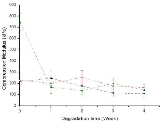
4.3.2. Mechanical Properties

The results achieved for the mechanical properties are shown in Figure 4.8. In the appendix (section 6.3), detailed results can be seen, in Table 6.3 and Figures 6.4 to 6.6.

Figure 4.8 – Compression moduli evolution throughout the degradation time, for () HMw, (▲) MMw and (■) LMw CS.

In a general way, compression modulus decreased throughout degradation time. Incomplete washing of the samples can be an explanation for the exceptions, once again. Additionally, all ICC with low molecular weight exhibited a brittle behaviour, which hampered sample handling during the compression tests, causing the loss of several ICC, making it difficult to obtain reliable results.

Moreover, for the same degradation time, excluding non-degraded samples, compression modulus did not seem to show a significant dependence on the molecular weight.

This result is not in good agreement with what was expected. Usually, higher molecular weight confers higher mechanical properties. However, in this case there is another parameter to consider: the concentration used in the impregnation solutions for each case. Lower molecular weight ICC possess a

(42)

22

higher concentration, meaning that there is a higher amount of polymer in the structure, which also influences mechanical strength.

Comparing H0 with M0 the compression modulus increase is once again not significant. However, comparing L0 with M0 and H0, it is possible to observe that the values of the compression modulus tripled. In this case, one can conclude that the effect caused by increasing the polymer mass prevailed, especially in the low molecular weight samples.

It is important to stand out that some measurements possess a high relative standard deviation (especially H0) and, for this reason, do not have statistical significance.

An abrupt decrease in the compression modulus for the LMw ICC submitted to degradation tests is clear in Figure 4.8, emphasizing the devastating effect of the degradation in these samples. However, it is important to stand out that the results from weeks 1 to 4 might not be completely reliable, since most LMw samples were lost or partially damaged during handling.

In order to support the results for the compression modulus of the ICC, compression tests were carried out in freeze-dried “bulk” scaffolds. These scaffolds were produced by pouring solutions with the same concentration as the ones used for CC impregnation in a 48 well culture plate. The compression tests were performed after freeze-drying and the results can be consulted in Figure 4.9 and Table 6.4 (appendix – section 6.3).

Figure 4.9 - Compression modulus evolution with the molecular weight of the chitosan, in (■) freeze-dried scaffolds and in () ICC.

Based on Figure 4.9, one may conclude that the evolution of the compression modulus with the molecular weight is similar for both lyophilized and ICC scaffolds. These results corroborate the previous conclusions, pointing out the prevailing effect of a higher amount of polymer over the effect of a higher molecular weight in mechanical properties in the LMw case.

(43)

23

Analyzing Table 6.3 (appendix – section 6.3), one can see that the compression moduli range from 108 kPa to 747 kPa, significantly higher than the values obtained by Choi et al. (30-60 kPa) [1]. However, considering the compressive strength of bone is between 4 and 12 MPa (Table 6.5, appendix – section 6.3), one can conclude that the values obtained for the ICC are too low for the application. Therefore, it is necessary to increase the mechanical strength, which can be achieved by incorporating a reinforcement in the chitosan matrix, such as hydroxyapatite or other calcium phosphates. Chitosan reinforcement with calcium phosphates, as a solution to increase mechanical strength, has already been successfully achieved in different scaffolds [13,36].

4.3.3. Morphological Characterization High Molecular Weight ICC

In Figure 4.10, it is possible to observe the morphology of a non-degraded HMw ICC, in which the walls are extremely porous, due to the small amount of polymer present in the impregnation solution. Lower amount of polymer leads to high porosity and structural instability, which results in a lack of organization due to the microsphere leaching stage.

Figure 4.10 – SEM image of a non-degraded high molecular weight CS ICC.

Poor mechanical properties, achieved for HMw ICC, reflect inadequate structural organization and high porosity.

(44)

24

Figure 4.11 – SEM images of high molecular weight samples with (a) one, (b) two, (c) three and (d) four weeks degradation.

The only sample from week 1 of degradation (Figure 4.11 (a)) collapsed during the washing steps, very frequent in HMw samples. For that reason, the referred image will not be considered for further analysis.

Although the mass loss results prove that degradation is effective from the first week, in high molecular weight samples, the effects of degradation become visible only in the third week. From the second to third week it is notorious that the initially non-porous walls at the surface begin to wear out, getting thinner. Within the pores, it is also possible to observe a clear increase in the porosity. The degradation effects become more severe in the fourth week, when the walls begin to collapse and the structure starts to lose its characteristic geometry. Besides the increase of porosity in the hollows, it is possible to observe the presence of pores in the wall ate the surface, which were not visible in the first three weeks of degradation.

Medium Molecular Weight ICC

In Figure 4.12, it is possible to observe the morphology of a non-degraded MMw ICC, in which the walls are highly porous, once again. However, it is possible to observe a nearly HCP arrangement, suggesting that the structure possesses an improved organization, mainly due to a higher resistance to the washing step, conferred by a higher amount of polymer.

(45)

25

Figure 4.12 - SEM image of a non-degraded medium molecular weight CS ICC.

Figure 4.13 – SEM images of medium molecular weight samples with (a) one, (b) two, (c) three and (d) four weeks degradation.

Although the degradation effects are visible right from the start (see Figure 4.13), the structure maintains its original shape until the end of the four weeks. This can be explained by the fact that the walls contain a higher amount of chitosan, since the impregnation solution had a higher initial concentration.

Low Molecular Weight ICC

In Figure 4.14, it is possible to observe the morphology of a non-degraded LMw ICC. In this case, the structure exhibits much lower porosity in the CS walls, due to a significant increase in the

(46)

26

concentration of the impregnated solution. Moreover, the HCP arrangement is much clearer, due to an improved resistance to the washing stage, conferred by the higher amount of polymer

Figure 4.14 - SEM image of a non-degraded low molecular weight CS ICC.

Summarizing, the mechanical performance of the non-degraded ICC was mainly influenced by two features: molecular weight and amount of polymer impregnated.

Higher molecular weights typically lead to higher mechanical properties, since longer polymer chains have less mobility, which makes it harder to deform [37]. Otherwise, incrementing the polymer mass in the walls, which happened for lower molecular weights, leads to the production of denser walls and improved structural organization, which also confers higher mechanical strength.

Figure 4.15 – SEM images of low molecular weight samples with (a) two, (b) three and (c,d) four weeks degradation.

(47)

27

All the LMw samples from the first week of degradation disintegrated during handling, which made it impossible to obtain SEM images.

By the second week, there are already several shattered walls (see Figure 4.15 (a)). In the third week, the sample is so degraded that it becomes difficult to differentiate the ICC pores. In the last week, there are fully degraded regions, visible in Figure 4.15 (d), in which the ICC identity is completely lost.

These observations support and somehow explain the unexpected mechanical behaviour of the LMw samples. Although LMw ICC exhibited higher initial compression moduli, it was also observed that these structures acquired a brittle behaviour and a rapid decrease in mechanical properties after one week of degradation. The increasing porosity and structure destruction, evident when comparing Figures 4.14 and 4.15, supports such an abrupt decrease.

4.3.4. Porosity

In theory, an ICC’s porosity should match the CC’s packing fraction. However, it is necessary to take into account that chitosan also possesses porosity, after freeze-drying, which increases the porosity value.

From the porosity determined for a CC in section 4.1.4. (29%), one can conclude the packing fraction is about 71%, which means that a chitosan ICC has more than 71% porosity. In this section, the main objective was to quantify the evolution of the porosity throughout degradation time, already noticed in the SEM images from the previous section.

The first method involved determining the ICC mass in three different situations: dry state (𝑚𝑑),

hydrated (𝑚ℎ) and submerged in water (𝑚𝑖). Then, using equation 4.1, it was possible to obtain the open

porosity values [38].

As an ICC is made of chitosan, it absorbs water not only in the pores, but also between the polymer chains [39]. This way, using this method, the values obtained for the porosity were absurdly high.

The second method was based on the Gibson and Ashby model for cellular solids [40]:

𝐸 𝐸𝑠≈ ( 𝜌 𝜌𝑠) 2 (4.3) where E is the Young modulus and  is the density for the scaffold and Es and s represent the same parameters for a solid produced with the same material.

Freeze-dried scaffolds where considered to be the “solid” and their mechanical properties and density were measured in the same conditions as the scaffolds. The results can be consulted in Table 6.6, in the appendix, section 6.4.

This time, the results were lower than expected, exactly because the freeze-dried scaffolds were considered a solid (without porosity). As mentioned before, by freeze-drying chitosan solutions, the final structure acquires pores, which result from the sublimation of water crystals. Therefore, the obtained results were lower than expected, as freeze-dried chitosan’s porosity was not considered.

Although the results are not good enough to quantify the porosity evolution, it was possible to observe an increasing porosity tendency along with the degradation. Additionally, H0 and M0 samples both have higher porosity values than L0, which is in good agreement with the results from the morphology section.

(48)

28

4.3.5. Cell Culture Cell Adhesion

Cell adhesion results, shown in Table 4.4, were achieved by the resazurin method. As the ICC did not covered the entire well area, some of the cells were unintentionally deposited on the well surface when the medium culture was poured. For this reason, a percentage of the 30000 cells placed in each well attached to the plate rather than to the ICC. Therefore, to determine the absorbance equivalent to cell adhesion, it was necessary to previously remove the ICC from the original well to a new one without cells, in order to have the resazurin converted in resorufin exclusively by the cells adherent to the ICC.

Table 4.4 – Cell adhesion after 24h, for different molecular weight ICC.

Sample Cell adhesion (%)

H0 45.3

M0 35.5

L0 20.0

High molecular weight ICC showed the best cell adhesion, followed by MMw. Low molecular weight scaffolds exhibited a considerably lower adhesion percentage.

Cell Proliferation

Evaluation of the number of cells in each well is made using the cell viability indicator resazurin that is reduced into resorufin by living cells. Resazurin is a blue compound with an absorbance peak at 600 nm, while resorufin is a red compound with an absorbance peak around 570 nm. Absorbance measurements can quantify the conversion of resazurin in resorufin, which is proportional to the number of metabolically active cells, while keeping the cells viable [41]. Thereby, it becomes possible to evaluate cell proliferation throughout time. Absorbance measurements obtained during the experiment are shown in Table 6.7 (appendix – section 6.5) and the evolution of the results can be observed in Figure 4.16.

Figure 4.16 – Absorbance evolution throughout SaOs-2 culture time, for HMw, MMw and LMw ICC.

Considering that absorbance values are proportional to the number of viable cells, one can see HMw and MMw scaffolds exhibit cell growth during cultivation, which suggests optimal biocompatibility

0 0,05 0,1 0,15 0,2 0,25 0,3 1 3 6 8 10 Ab s o rv a n c e

Culture time (Day)

L0 M0 H0 LMw MMw HMw

(49)

29

[42]. Medium molecular weight samples showed a slightly higher growth trend from the beginning. This behaviour was emphasized in the last cultivation days, resulting in a reasonably higher absorbance for MMw ICC, which indicates a larger number of cells. After 10 days, both MMw and HMw absorbances revealed a six fold increase. However, low molecular weight ICC results suggested almost complete cellular death by day 8. Molecular weight is the only difference between the ICC sets, which does not appear to be an adequate explanation for such a difference in cell behaviour. It is possible that these results are due to improper sample handling during resazurin tests.

Optical and scanning electron microscopy observations of the different samples, present in Figures 4.17 to 4.20, are in good agreement with the reported results.

Figure 4.17 – MO images of different regions of a HMw ICC, exhibiting some cell agglomerates (bright dots).

Figure 4.18 - MO images of the same area of a MMw ICC, with different focus ranges, exhibiting cell agglomerates all over the structure.

(50)

30

Figure 4.19 - MO images of the same area of a LMw ICC, with different focus ranges, showing no visible cells.