E
QUITY
V
ALUATION USING
A
CCOUNTING
N
UMBERS
IN
D
IVIDEND AND
N
ON
-D
IVIDEND
P
AYING
C
OMPANIES
Candidate:
Alexandra Kleba
Advisor:
Dr. Ricardo Reis
Dissertation submitted in partial fulfilment of requirements for the degree of MSc in Business Administration, at the Universidade Católica Portuguesa
III
ABSTRACT
The aim of this thesis is to understand how firms with different payout policies impact the performance of equity valuation models and what characterizes them. After introducing theory regarding pertinent models and reviewing relevant literature, flow and stock-based model performances are analyzed across two large subsamples of US firms, dividend and non-dividend paying firms. The first group shows a better performance in general while a higher performance discrepancy between both subsamples is visible amongst the best performing models. This alerts the user of the fact that models value firms differently according to their payout ratio. Building on this breakdown, a small sample analysis, between two subsamples of UK firms, analyzes not only the models used by brokers’ reports in reality but also other relevant variables. The most pronounced differences are the firms’ size, investment opportunities, equity models used and brokers’ recommendation.
IV
I
TABLE OF CONTENTSI Table of Contents ... IV II List of Tables ... VI III Abbreviations ... VII
1 Introduction ... 1
2 Review of Theory and Relevant Literature ... 2
2.1 Informational Content of Accounting Numbers ... 2
2.2 Theoretical Models ... 3
2.2.1 Stock-Based Valuation Models (Market Multiples) ... 4
2.2.1.1 Selection of Comparable Firms ... 5
2.2.1.2 Selection of Relevant Value Driver ... 5
2.2.1.3 Computing the Benchmark Multiple ... 6
2.2.2 Flow-Based Valuation Models ... 7
2.2.2.1 Discounted Dividend Model (DDM) ... 7
2.2.2.2 Discounted Cash Flow Model (DCFM)... 8
2.2.2.3 The Residual Income Valuation Model (RIVM) ... 9
2.2.2.4 Ohlson/Juettner-Nauroth Model (OJM) ... 11
2.3 Empirical Evidence ... 12
2.3.1 Empirical Evidence on Stock-Based Valuation Models ... 12
2.3.2 Empirical Evidence on Flow-Based Valuation Models: ... 14
2.4 Concluding Remarks ... 16
3 Dividend and Non-Dividend Paying Firms ... 17
3.1 Introduction ... 17
3.2 Review of Relevant Literature ... 17
3.3 Concluding Remarks ... 21
4 Large Sample Analysis ... 23
V
4.2 Hypothesis ... 23
4.3 Valuation Models ... 23
4.4 Research Design (Data and Sample) ... 24
4.5 Empirical Results ... 27
4.5.1 Descriptive Statistics ... 27
4.5.2 Significance Level Tests ... 29
4.5.3 Univariate Regression ... 30
4.5.4 Robustness Test ... 31
4.6 Concluding Remarks ... 33
5 Small Sample Analysis ... 35
5.1 Introduction ... 35
5.2 Hypothesis ... 35
5.3 Tested Variables ... 36
5.4 Research Design (Sample and Data) ... 36
5.5 Empirical Results ... 38
5.5.1 Descriptive Statistics ... 38
5.5.2 Significance Level Tests ... 40
5.6 Concluding Remarks ... 41
6 Conclusion ... 42
IV Reference List: ... 44 V Appendix ... IX
VI
II LIST OF TABLES
Table 1 – Sample Selection Procedure……….………...…25
Table 2 – Sample Characteristics………...…25
Table 3 – Descriptive Statistics, Valuation Errors………...28
Table 4 – Comparison of Bias/Accuracy Prediction Errors between/within Sample Partitions………..…….30
Table 5 – Univariate Regression of Stock Price on Value Estimates…...…31
Table 6.1 – Robustness Test, Descriptive Statistics………..….32
Table 6.2 – Robustness Test, Comparison of Bias/Accuracy Prediction Errors within Sample Partitions………...32
Table 6.3 – Robustness Test, Univariate Regression of Stock Price On Value Estimate……….……..….…..33
Table 7 – Industries, ICB Classifications………...………37
Table 8 – Sample Selection……….……38
Table 9 – Descriptive Statistics……….………..39
VII
III ABBREVIATIONS
AIG abnormal income growth
book value of equity
B/P book value-to-price
C operating activities of the company CRSP Centre for Research in Security Prices
C-I free cash flow
d dividends
DCFM discounted cash flow model DDM discounted dividend model
D/P dividends-to-price
EPS earnings per share
EV enterprise value
EV/S enterprise value-to-sales E(DPS) expected dividend per share E(NI) expected net income
g growth rate
I amounts invested in the operating activities of the company ICB industry classification benchmark
IPO initial public offering
I/B/E/S Institutional Brokers' Estimation System
ke cost of equity
VIII NPV net present value
OJM Ohlson/Juettner-Nauroth model OLS ordinary least squares
P/B price-to-book
P/E price-to-earnings
RI residual income
RIVM residual income valuation model
R2 explainability
debt value equity value
V/P value-to-price
1
1 Introduction
This year Apple, an American multinational company that creates and sells consumer electronics, personal computers and computer software, paid its first dividend over a decade. The payout marks a big shift for the company which after a near bankruptcy in the 90’s had not paid a dividend since.
The shift of these and other companies from non-dividend paying firms to dividend paying firms raises the question of what triggers a firm to pay out dividends. Consequently, if firms decide to change their payout policies then these firms’ characteristics most probably changed over the years setting off a new policy. The mean of this analysis in hence to study dissimilarities across these two types of firms under the light of equity valuation using accounting numbers.
In a large sample analysis, accounting-based valuation methods estimate dividend and non-dividend paying firms’ value, presenting the superior valuation models for each subsample. Besides ranking the models according to their performance, this analysis shows where the discrepancy between groups is most pronounced.
Then, a small sample analysis examines the differences amongst these subsamples within a selection of brokers’ reports. Besides outlining which models are used by practitioners in reality this analysis studies other variables that can hardly be collected from electronic databases.
Broadly, this thesis pursues the following structure: the subsequent section presents models relevant literature for equity valuations using accounting-based valuation models. Besides pointing out advantages and disadvantages, their relevance given the study intend is presented. Section 3 focuses on literature review and empirical findings from firms with different payout ratios specifically. Section 4 delivers the results of the large sample analysis while section 5 focuses on a small sample of analysts’ reports. Section 6 concludes the thesis with a summary of main results and suggests fields of further research.
2
2 Review of Theory and Relevant Literature
2.1 Informational Content of Accounting Numbers
Starting by explaining the need for equity valuation, this chapter follows with the introduction of both perspectives valuations can be conducted from and finishes by presenting a brief literature review on the informational content of accounting numbers.
Equity valuation relies on transforming forecasts of key variables into a value estimate (Penman, 2003). Undergoing this procedure might be questionable since obtaining the share price is the purpose of this operation and the share price is mostly available in a market that is assumed to be efficient (Malkiel, 1989).
Quoted share prices might, however, in some cases be insufficient. Private businesses that are not quoted and need to be valued for IPO’s or acquisitions require equity valuations. If a company develops a strategy internally and the management intends to test its impact on the current value, equity valuation is necessary. Finally, equity valuation is also applied to verify if companies are correctly priced (Damodaran, 2002). Assuming that markets are efficient does not mean that all stocks are constantly correctly priced (Malkiel, 1989). Equity valuation provides in these cases a reality check on forecasts implied by market prices.
A firm’s valuation can be implemented through two points of view, the entity perspective and the equity perspective. The entity perspective neglects the source of funding to finance the operating assets. It values the operating entity as a whole, combining debt and equity shareholders’ funds. The equity perspective distinguishes between capital provided by shareholders and debt holders, focusing on the first one. Valuations can be conducted from either perspective, moving from one to the other by adding or deducting the capital provided by debt holders (Citigroup Global Markets, 2008).
Accounting data has not always been seen as a useful tool. Versions of the argument that income numbers lack meaning and are consequently of
3 questionable utility appear in Canning (1929); Gilman (1939); Paton and Littleton (1940), among others.
Ball and Brown (1968) argue that this line of thought is mainly based on the constant development of accounting practices facing new incidents. The inexistence of an identical cross-border framework creates divergences in accounting practices, making net income figures inconsistent. Being aware of these differences, but also of the fact that net income is a number of particular interests for investors, Ball and Brown analyze the net income significance in terms of content and timing and conclude that of all the information becoming available about a firm over the year, most is captured in that year’s income number. The net income content is therefore considerable. In this study net income is, however, not considered a timely medium, once most of its information is captured in other, more timely, media such as interim reports. Beaver (1968) addresses the same issue by examining the extent to which common stock investors perceive earnings to have informational value. He particularly focuses towards the investor’s reaction to earnings announcements in terms of volume and price movements of common stock in the weeks nearby the announcement date. According to his approach there are two main reasons to believe that earnings lack information value. First, measurement errors in earnings are too large and second, even when earnings convey information there are other sources available to investors that contain the same, but timelier, information. During his analysis, Beaver observes a price reaction as well as a volume reaction, indicating that not only expectations on individual investors are altered by the earnings report, but also the expectations of the market as a whole.
Both papers conclude that even though accounting numbers might not be the ideal source of information, they are still the best available alternative and extremely important for investors and equity valuations.
2.2 Theoretical Models
There are many approaches for equity valuations, from very detailed analyses to rather simple implementations. The ones that matter for this review are the
4 stock-based valuation models and within the flow-based valuation models: the discounted dividend, the residual income valuation and the Ohlson/Juettner-Nauroth model, due to their international spread and acceptance.
Given the aim of this study, theoretical models and later presented empirical evidence are analyzed in terms of their contribution towards the research intend, shedding a light on how models and findings influence the performance of firms with different payout ratios.
2.2.1 Stock-Based Valuation Models (Market Multiples)
Fundamental analysis is detailed and costly so a simple approach is sometimes preferable avoiding forecasting and minimizing information breakdown (Penman, 2003). One of the most common methods is the market multiples method.
As Penman (2003) points out, the multiples method starts by identifying firms that have similar characteristics to the firm that is seeking to be valued, the target firm. After identifying the comparable firms it is time to identify measures or value drivers in their financial statements and compute benchmark multiples of those measures at which the firms trade. Finally the calculated benchmark multiples need to be applied to the corresponding measures for the target to estimate that firm’s value.
The general method for price multiples can be written as follows:
The multiple-based valuation can either be implemented through equity-level or entity-level multiples. The reason to choose one perspective over the other depends on the company being considered. In case accounting and financing policy differences make comparing equity multiples difficult or when non-core businesses distort comparability, then the use of enterprise-value (EV) multiples is preferable. Relying on equity multiples is encouraged, when EV multiples are less meaningful or when additional forecast inputs want to be avoided (Citigroup Global Markets, 2008).
5 Despite its apparent simplicity, multiple-based valuation requires complex decision making processes which are described below.
2.2.1.1 Selection of Comparable Firms
The first implementation issue is the selection of comparable firms. The goal is to find one or several firms that best represent the target firm. The advantage of choosing a single comparable firm is that the probability of identifying a closer match of the target firm is higher. A set of firms, however, provides the benefit of canceling out firm specific characteristics leaving only average factors. One possible approach is to select comparables operating in the same industry, which are more likely to be affected by the same set of factors, being the most closely related to the firm being valued. In case an industry is, however, not well defined, the intra-industry differences can be significant, making the comparable selection difficult (Penman, 2003).
2.2.1.2 Selection of Relevant Value Driver
The second implementation issue is the selection of the most appropriate value driver. The principal criterion is to choose the value driver that is most closely correlated with value/price relation. Based on the fact that accruals help overcome the timing and mismatching problems inherent in cash flows, tied with the reality that current earnings provide a more reliable prediction for future cash flows than current cash flows, earnings are generally the preferred value driver (Liu et al., 2002).
Some multiples, including the Price/Earnings (P/E) multiple, are affected by leverage. Unless it can be assumed that the leverage of the comparable and target firms are similar, it might be sensible to use P/E ratio formulations that focus on entity-level value drivers rather than equity-level value drivers (Penman, 2003).
Finally, the selected value driver should, when using an earnings value driver, rather be a forecast of profits than a historical profits figure. Following the theory of finance, the value of an asset depends on the stream of expected future cash flows. The correlation between the firm’s price, the expected future cash flows,
6 and the expected future profits is likely to be higher than the correlation between the firm’s price and historical profits figure (Penman, 2003).
2.2.1.3 Computing the Benchmark Multiple
The final implementation issue is the computation of the benchmark multiple. The calculation of the benchmark multiple is a crucial step in this valuation method as it highly influences the target firm’s value (Liu et al., 2002). Calculating the arithmetic average is one possibility.
The problem in implementing this option is the possible existence of outliers. Outliers are often encountered in accounting research and influence the mean considerably. Alternative calculations that alleviate this problem are the use of the median or the weighted average. A third alternative would be the use of the harmonic mean, the reciprocal of the mean of the reciprocals of the ratio. The harmonic mean diminishes the effect of small denominators as well as it yields less upward-biased estimates. Note that in any of the presented possibilities the target firm is always excluded from the comparable group when estimating its benchmark multiple (Liu et al., 2002).
Summarizing, the multiple-based approach owes its popularity to its simplicity and its absence of multiyear forecasts of parameters. Users rely on the market to undertake the task of forecasting. The success of this valuation method relies on the assumption that future cash flows and risk profiles of comparables firms are similar to the target firm and that the value driver is proportional to value (Damodaran, 2002). This approach can however not safeguard against a sector or even the market being wrongly priced.
The use of this method is adequate for the aim of this study as it allows firms with different payout ratios to be valued. Given the properties of this method, similar firms in terms of business strategy, operational sector as well as dividend policies can be selected as comparable firms, enabling an adequate valuation for each firm.
7
2.2.2 Flow-Based Valuation Models 2.2.2.1 Discounted Dividend Model (DDM)
The DDM, attributed to Williams (1938), values a firm’s intrinsic equity value by forecasting and discounting future dividends. The model discounts future dividends ( ) at the cost of equity giving ( ) rise to the firm’s present value ( ).
Forecasting infinite future flows is highly impracticable. As a result, valuation models using forecasts of flows often comprise these up to a certain horizon and establish then a continuing-value term. This continuing-value term can then assume two scenarios. One possible assumption is expecting the firm to pay the same dividend to infinity, neglecting any growth factor after the horizon time. Assuming that the firm pays dividends that are a growing perpetuity is the second scenario, also known as the Gordon growth model (Damodaran, 2002). Finally, by multiplying the value per share by the number of shares, the Firm’s equity value is calculated.
Value per share of stock (no growth):
Value per share of stock (growth = g):
At first sight this model seems to be very appealing. Based on an easy concept it forecasts what shareholders get. Once dividends are usually relatively stable, in the short run, they are fairly easy to forecast. At a closer look this model reveals, however, some shortcomings. A company’s dividend policy is not directly linked to value added and can instead be arbitrary. A company can increase its leverage to pay dividends, while not creating value. Dividends represent hence the distribution of wealth, rather than the creation of wealth. Moreover, flow based valuations require forecasts for long periods. A company’s dividend policy can be stable in the short run, but it is not very
8 predictable in the long run, incorporating easily errors in estimating key ingredients. Finally, the DDM only applies to companies that pay out dividends. There are, however, many firms that do not pay out dividends. In these cases, the application of this model is not possible (Penman, 2003).
Summarizing, this model is not always applicable, but it works best when a company’s payout is permanently tied to the value generation of the firm, such as when a firm has a fixed payout ratio (Penman, 2003).
With the aim of comparing the performance of firms with different payout ratios for several valuation models, this method shows to be inadequate. Once the valuation model relies on dividends, non-dividend paying firms are automatically not valuable through this method. Hence, a comparison between groups’ performance (dividend and non-dividend paying) is here impossible.
2.2.2.2 Discounted Cash Flow Model (DCFM)
The intrinsic value of equity can be calculated directly by forecasting cash flows to equity holders, as presented by the DDM. Alternatively, the value of equity can be estimated by forecasting the free cash flow (the value of the firm), arising from the operating activities of the company, C, net of amounts invested in the operating activities, I, followed by the deduction of the debt value ( )
(Penman, 2003). The DCFM estimates hence the value of the firm rather than the equity’s intrinsic value and requires therefore the subsequent deduction of the firm’s debt. The DCFM is one of the most accurate and flexible methods for valuing projects, divisions or even entire companies. Any analysis is, however, only as accurate as the forecasts it relies up on, highlighting the importance of the right free cash flow forecasts as well as of the appropriate weighted average cost of capital (Copeland et al., 2000).
After forecasting a firms free cash flows (C-I) these are discounted at the weighted average cost of capital (WACC), the cost of capital for the entity perspective.
A terminal value is assumed, avoiding infinite free cash flow forecasts, which can either represent a flat or growing perpetuity.
9 Equity Value (no growth):
Equity Value (growth):
The DCFM owes its popularity to its familiar concept and its detailed analysis. Cash flows are not affected by accruals and are therefore easily considered. The same model incorporates nevertheless some weaknesses. The DCFM does not measure value added over the short run. If a firm invests more cash in operations than it makes from operations, the free cash flow is negative even if the NPV of the project is positive, treating investment as a value loss. In the long run the free cash flow will be positive but the greater the current investment is, the longer the forecasting horizon has to be to take into consideration these cash inflows. A highly extended forecasting horizon results then in less accurate forecasts and threatens the valuation estimate precision. Also, the DCFM is a highly liquid concept. A firm’s free cash flow increases as soon as the investments are cut. This, results in a higher value estimate even if investments are reduced (Penman, 2003). Additionally, this model is not aligned with what professionals forecast. Analyst forecast earnings, not free cash flows. As Damodaran (2002) points out, the use of this model requires therefore further adjustments to convert earnings into free cash flows. Finally, this model is unsuccessful in recognizing value that is not incorporated directly in cash flows. Summarizing, this model values firms with different payout ratios, providing a more detailed analysis of the firm’s intrinsic value. Due to its limitations Penman (2003) suggests the model is best applied to companies whose investment pattern produces a stable free cash flow, such as cash cows.
2.2.2.3 The Residual Income Valuation Model (RIVM)
Being already mentioned by Preinreich (1938) and Peasenell (1982) the RIVM is not a new discovery, nevertheless it was recently revived by the work of
10 Ohlson (1995) and Feltham and Ohlson (1996) resulting in an outburst of interest.
Feltham and Ohlson (1999) base the usefulness of this valuation method on the focus shift from wealth distribution, dividends, to accounting measures of wealth creation, book value and abnormal earnings. The wealth creation depends therefore only on the firm’s activity as opposed to the financing of those activities. As shown in Appendix 1, the RIVM is derived from the essential expression of the DDM. Equity Value: Residual Income:
As presented in the equation above, the equity perspective application of the RIVM involves the observation of the accounting book value of equity and the forecasted residual income discounted at the cost of equity, including a continuing value term. Residual income, also known as abnormal earnings, are the earnings in excess of a normal return on capital employed (Penman, 2003). Alternatively, the model can be applied from the entity perspective, adjusting the equity perspective items to entity perspective items.
This valuation model comprises an anchor, the book value, and a premium over the book value, the present value of forecasted residual income (Ohlson, 2005). Consequently, if a firm expects to earn a normal rate of return on the capital employed, the intrinsic value of the firm equals the book value of equity, including no premium, from the equity perspective. If, however, the company expect to earn more than a normal return on capital employed the equity value will exceed its book value. The same applies to the entity valuation method. The strength of this model, applicable to firms with any kind of payout ratio, relies on using the value component recognized in the balance sheet, the book
11 value, which does not form part of the forecast-flow component. Additionally, the RIVM uses properties of accrual accounting. These properties recognize value in advance, matching value added to value given up. Contrary to the DCFM, the RIVM treats investment as an asset instead of a cost, resulting in smoother series of cash flows. Consequently, the forecast horizon for this model is shorter than when using the DCFM (Penman, 2003).
The downside of this model is its accounting complexity (Penman, 2003). Requiring some understanding of how accrual accounting works is necessary to facilitate the identification of causes of concern. Also, residual income is not a natural focus of attention for analysts which are more familiar with the use of forecasted earnings. Finally, this model relies on clean surplus accounting while existing literature recognize that GAAP’s earnings construction violate the clean surplus relation (Ohlson, 2005).
2.2.2.4 Ohlson/Juettner-Nauroth Model (OJM)
The Ohlson/Juettner-Nauroth (OJ) Model, also known as the Abnormal Income Growth (AIG) Model, is derived from the DDM as shown in Appendix 2 (Ohlson & Juettner-Nauroth, 2005). The intention is to overcome some shortcomings presented by the RIVM by replacing the anchor used in this model, the current book value, with the subsequent period capitalized earnings (Ohlson, 2005). Additionally, to estimate the firm’s equity value, the present value of capitalized abnormal income growth (AIG) of next-periods, where AIG is the difference in income minus the normal return on previous-period retained income, is added. Equity Value: Where
Note that also the OJM can be written in terms of the entity perspective by adjusting the equity perspective items to entity perspective items.
12 Analyzing this model it appears to have some advantages over the previously presented RIVM. When looking closely at the anchor term it is visible that the capitalized next-period income can be rewritten as current book value plus capitalized subsequent period residual income.
OJM Anchor from equity perspective:
Compared to the RIVM anchor it is clear that the OJM anchor incorporates a larger portion of value, making the terminal value less influential. Additionally, this model does not rely on clean surplus. Then, focusing on income cannot be worse than to focus on book value, but the reverse is false, as stated by Ohlson (2005). Ohlson argues also that capitalized income approximates market values more closely than book values. Finally, investment practices rotate around income and their growth, not book value and their growth, (Penman, 2003). The use of this model requires, however, an understanding of accrual accounting (Penman, 2003). The forecast horizon in the OJM might be shorter than the one for the DCFM but the forecasts do depend on the quality of the accrual accounting.
2.3 Empirical Evidence
2.3.1 Empirical Evidence on Stock-Based Valuation Models
Multiples and their implementation issues have been a major focus for published papers by Boatsman and Baskin (1981), Alford (1992), Kaplan and Ruback (1995), Kim and Ritter (1999), Baker and Ruback (1999), amongst many others. Most of these papers perform their examination, however, only over a limited period of time and consider merely a subset of multiples. Additionally, as the methodology differs across studies a comparison between those is difficult.
The focus will therefore shift to the paper published by Liu et al. (2002). This paper focuses on how the accuracy of multiple-based valuation varies when it is
13 specified differently: across different peer groups, across different value drivers and across different estimations of the benchmark multiples.
The primary focus is the traditional approach, assuming direct proportionality among price and value driver, selecting comparable firms based on their industry. In a further stage a less restrictive approach is considered, allowing for an intercept and expanding the group of comparables to the whole sample. To avoid negative predicted prices, the authors restrict their sample to positive multiples, eliminating negative firm-years in general (Liu et al, 2002, p. 145). The multiples used in calculating the pricing errors during this study are estimated using the harmonic mean. To make results comparable with other studies (e.g. Alford (1992)) the procedure is repeated using the median. In line with results in Baker and Ruback (1999), the multiples performance is worse when making use of the median as opposed to when using the harmonic mean. The study finds that multiples based on forward earnings explain stock prices relatively well for the majority of the sample. Historical earnings are ranked second, book value and cash flow measures are the third best alternative and sales-based have the worst performance. Contradicting findings from Tasker (1998), this ranking is consistent across several industries and across a wide time range. Selecting companies from the same industry seems to improve the performance of all value drivers and relaxing the restriction, allowing the use of an intercept, improves mostly measures that performed worse previously. Note that, due to the imposed restrictions on forecasts and positive values, the results might not representative for firm-years excluded from the sample. The sample is unlikely to contain emerging technology firms such as Internet stocks (Hand 1999, 2000).
A different implementation issue is analyzed by Bhojraj and Lee (2002). Bhojraj and Lee suggest that comparable firms should be identified in accordance to a measure, the warranted multiple, rather than selecting comparables based on industry or size. This measure combines characteristics specific to the target firm and the market association between these characteristics and the multiple. For each target firm its comparables are hence the ones whose warranted multiples are the closest to the warranted multiple of the firm under analysis.
14 During their study, Bohjraj and Lee restrict their analysis to only two valuation multiples: the Entity Value/Sales (EV/S) and the Price/Book (P/B) multiple. The reason for selecting these two multiples is based on the fact that these are highly unlikely to adopt negative values.
The authors compare this approach to traditional approaches selecting comparables based on their industry and size. Bohjraj and Lee conclude that comparable firms selected through a similar warranted multiple perform better relative to traditional comparable firm selection methods, improving significantly the valuation outcome.
Considering this finding, it is important to remember that the implementation of complex warranted multiples improves the outcome, compromising however the simplicity multiples owe its popularity to.
2.3.2 Empirical Evidence on Flow-Based Valuation Models:
To study the performance of different flow based valuation models Francis et al. (2000) examine the value estimated of three theoretically equivalent valuation models. Several studies examined flow based methods previously such as Kaplan and Ruback (1995), Frankel and Lee (1995; 1996), Bernard (1995), but particularly Penman and Sougiannis (1998). Knowing that Penman and Sougiannis (1998) had performed their analysis on realized portfolio payoffs and signed prediction errors, Francis et al. (2000) base their study on forecasted payoffs of individual securities and extended their focus on accuracy and explainability.
Driven by the question of which model to use to measure a firm’s intrinsic value the authors examine three flow based models: the DDM, the DCFM and the RIVM. In line with previous studies, the results show that the RIVM consistently outperforms the DDM and the DCFM in terms of aggregation, type of data and performance metric.
This constant superiority of the RIVM might be based on the book value implementation, containing not only a flow based component, but also a stock component. This superiority holds as long as distortions in book values resulting
15 from management discretion are less severe than forecast errors in growth and discount rates. Alternatively, the superiority might be a result of a greater precision in terms of residual income forecasts.
With the outburst of interest in the role of the RIVM due to the works of Ohlson (1995) and Feltham and Ohlson (1995), Frankel and Lee (1998) decide to compare different implementations of the RIVM. Frankel and Lee determine a value-to-price ratio (V/P), based on this model, to observe market efficiencies and predictability of cross-sectional stock returns.
They find that this V/P ratio outperforms the P/B ratio at explaining cross-sectional prices. Additionally, this ratio is a better predictor for long term returns. Also, a link between the V/P ratio and returns is established. High (low) V/P firms are linked to higher (lower) long term returns. The authors show that, taking advantage of these finding, an investment strategy based on buying high V/P stocks and selling low V/P stocks generates a 3 year cumulative return of 35%.
While the previous presented literature uses market prices as a benchmark for their analysis, Lee, Myers and Swaminathan (1999) compare the intrinsic value estimate of the RIVM (V) against other traditional models in terms of their tracking ability of price variation and their predictive power for future returns. The motivation of their study is to examine the autocorrelation and predictive power of future returns of the V/P ratio, based on the RIVM, against dividends (D/P), earnings (E/P) and book value (B/P) ratios.
During the analysis, the V/P ratio shows a smaller first-order autocorrelation, indicating a faster recovery when deviating from the mean, leading to the conclusion that the RIVM value estimate tracks the intrinsic value better than the other traditional models. Consistent with previous results, the V/P measures also outperforms the remaining measures in terms of significance power.
The study shows that earnings forecast methods and the risk free rate are the most important factors for the distinctive success of the RIVM. In line with previous findings Lee et al. (1999) conclude hence that time varying interest
16 rates and analysts’ earnings forecasts improve the performance of the V/P measures significantly.
2.4 Concluding Remarks
This review addresses the most common equity valuation methods, looking at the advantages and disadvantages of each method. Then, empirical research on these models is presented, concluding that in terms of the stock-based method the P/E ratio is the most recommended multiple followed by the P/B ratio. In terms of the flow-based models the RIVM consistently outperforms the other models. The OJM, a newly revived model, is not considered in most studies leaving its relative performance unknown.
With the aim of this study, the model that is inadequate to pursue further is the DDM. Its reliance on only dividend paying firms hinders any comparison between firms with different payout ratios. Also, empirical evidence suggests that for the later study market prices as benchmark of the analysis of different models are recommended as the tracking ability of price variations surpasses the scope of this analysis.
17
3 Dividend and Non-Dividend Paying Firms 3.1 Introduction
Each firm chooses if and how much dividends to pay its shareholders. Reasons that influence a firms’ willingness to pay out dividends might be based on the firms’ desire for stability, future investment needs, taxation factors, signaling effects or managerial interests (Damodaran, 2002).
The variability in dividends is lower than the variability in earnings as firms are unenthusiastic to change their dividend policy once the payout began. To prevent future cuts and with the uncertainty of future earnings, firms often reject a dividend increase, maintaining a constant or no payout policy at all. Additionally, if a company expects future investment opportunities its reluctance to pay out dividends decreases, once issuing securities might exceed the costs of keeping excess cash for future financing. Also, different tax rates might influence a firm’s payout rate. In case dividend gains are taxed at a higher rate than capital gains a firm might be more reluctant to payout dividends and vice versa. Furthermore, some argue, dividends often signal earnings quality, where a payout increase suggests a positive sign and a payout decrease, or no payout at all, suggests a negative sign. Finally, a firm’s payout decision might be influenced by managerial incentives. Retained earnings gives managers discretion to act in their interest and enables them to build up a cash cushion protecting their performance when earnings decrease (Damodaran, 2002).
3.2 Review of Relevant Literature
Given the complexity of this subject authors have, over time, come to different conclusions. It is the goal of this review to present the evolution of different findings, interpretations and theories issued by authors such as Modigliani and Miller, Fama and French, DeAngelo and DeAngelo, and many others.
Modigliani and Millers (1961) irrelevance theorem indicates that, in a frictionless market with a fixed investment policy, all capital structures and dividend policies are optimal. This suggests that any dividend policy implies identical stockholder wealth, making the choice among them irrelevant.
18 Several years later, DeAngelo and DeAngelo (2006) state that the only policy a firm can choose in Modigliani and Miller’s theorem is a 100% free cash flow payout. The authors propose that, contrary to Modigliani and Miller (1961), payout policy is not irrelevant and that investment policy is not the only value determinant in a frictionless market. Once retention is allowed dividend payout policy matters in the same way investment policy does. DeAngelo and DeAngelo (2006) also argue that the existence of benefits to retention do not eliminate the fact that these benefits must eventually be dominated by incentives for distribution. Hence, the suggestion of a trade off theory is made where flotation costs involved in issuing securities encourage retention and agency costs, managers and shareholders misalignment of interests, disencourage it.
DeAngelo and DeAngelo (2006) therefore conclude that firms in early years generate less internal capital then they have investment opportunities forcing them to rely on outside equity, hindering any payout policy. Firms in late years, however, usually have less profitable investment opportunities than internal generated cash, making agency problems appear. Given this scenario, firms mitigate opportunities for free cash flow waste paying out dividends.
Another striking finding was made by Fama and French (2001) documenting a major time-series change in dividend payout policy. In the time-span between 1978 and 1999, the percentage of firms that pay dividends decreased from 67% to 21%. Fama and French (2001) suggest that this decline is partly derived by the appearance of many small and unprofitable firms with strong growth opportunities. However, even after accounting for this trend Fama and French (2001) are still able to identify a considerable decline in the ‘propensity to pay dividends’, suggesting that even firms that pay dividends reduced their payout. Additionally, Fama and French (2001) state the difficulty to explain the reason for firms to pay out dividends, since dividends are taxed at a higher tax rate making firms who pay dividends suffer a competitive disadvantage. The authors make therefore use of logit regressions and summary statistics to identify the characteristics of dividends payers. Both analyses indicate that the decision to pay out dividends relies on three factors: profitability, investment opportunities
19 and size. Dividend paying firms are more profitable firms than non-payers, while non-payers have a higher investment rate. This finding seems to be consistent with the suggestion of Esterbrook (1984) and Jensen (1986) about the role of dividends in eliminating free cash flow agency costs. Finally, dividend paying firms are about 10 times larger than non-paying firms.
The appearance of new, small and unprofitable firms which do not pay dividends combined with the payout decline whatever their characteristics, due to deteriorating profitability, suggests a reduction in the alleged dividends benefits.
As possible explanations for dividends decline through time, Fama and French (2001) identify possibly lower transaction costs for trading stocks facilitating capital gains as well as better corporate government technologies controlling agency problems within a firm.
Intrigued by the question raised by Fama and French (2001), whether dividends are disappearing, DeAngelo et al. (2004) decide to take this analysis further. During their study, the authors discover that the final result is a significant decrease in the number of dividend payers, in line with Fama and French (2001), accompanied, however, by an increase in aggregate dividends. This finding indicates that the few top firms paying dividends dominate and increased the aggregate payout while the bottom firms have no or little impact on the dividend supply.
Supporting Linter’s (1956) findings, that firms’ dividend supply depends mainly on earnings, this suggests that the dividend concentration observed by DeAngelo et al. (2004) might be a result of significant earnings concentration. Also, knowing that the losses in 2000 exceeded the losses in 1978, found by Buegstahler and Dichev (1997), Fama and French (2001) and Ritter and Welch (2002), reinforce the fact that losses play an important role in dividend payout policy.
De Angelo et al. (2006) also question the empirical importance of signalling and clientele effect (Allen and Michaely, 1995). They argue that in case clientele effect was true, if investor were in fact attracted to different company policies, it
20 would be possible to see top firms not paying dividends across several industries and not only the technology industry. The fact that dividends are highly concentrated among a small number of prominent firms with high earnings, questions also the singling effect. The signalling effect suggests that companies rely on dividends to communicate to stockholder. If this theory were to be true, significantly smaller, relative unknown firms with limited access to financial press would recur to dividend payouts. The majority of firms recurring to payout policies are, however, important companies.
Given this discovery DeAngelo et al. (2006) decided to empirically test the life-cycle theory. The idea of this theory is that in young firms with many investment opportunities but limited resources, retention dominates distribution, while mature firms have fewer profitable investment opportunities and higher profitability, making them optimal dividend payers.
The idea, already introduced by Frama and French (2001), DeAngelo et al. (2004) and Grullon et al. (2002), hints at a life cycle theory where the benefits of payout policy (elimination of agency costs) dominate retention (elimination of floating costs) at a later stage. The puzzling finding, made by Fama and French (2001), suggesting that in recent years firms are much less likely to pay dividends than they were in the mid 1970s DeAngelo et al. (2006) explain by a shift towards a massive amount of firms with less earned earnings. A possible justification is given by Fink et al. (2004) stating that the age for a typical firm at its IPO date has fallen significantly from 40 years in the early 1960s to less than 5 years in the late 1990. Combining this fact with the evidence that new firms usually have less stable earnings and more growth opportunities, firms have become less likely to pay dividend because they are younger (DeAngelo et al., 2006).
Besides ruling out signalling and clientele effects, the authors now also rule out the catering incentives presented by Baker and Wurgler (2004). This theory argues that companies have incentives to pay dividends when the market overvalues dividend payments. The prediction of this theory is however inconsistent with findings by DeAngelo et al. (2006).
21 DeAngelo et al. (2006) argue that agency costs, implied in the life cycle theory, most powerful explain the reason for payout decisions of mature firms. The same conclusion, choosing the life-cycle theory as explanation for payout policies, Chahyadi and Salas (2012) reach in their study. At the end they raise, however, an additional question. The authors question whether the recent increase in share repurchases has an effect on the likelihood that firms pay dividends.
It is this same question that Jain et al. (2009) chose to examine in their analysis, comparing share repurchases with dividend payout policies. According to these authors, there is an ongoing debate about the extent to which share repurchases substitute dividend payments. By analyzing the differences in dividend paying and stock repurchasing firms, the authors are able to point out several significant differences between both groups.
Dividend paying firms are characterized by a higher leverage, profitability, maturity, sales and total assets, while the growth prospects are significantly lower. Additionally, these firms are less likely to be supported by venture capitalists. Hence, dividend paying firms follow generally the typical life cycle characteristics, favoring distribution over retention.
Stock repurchasing firms appear to have completely different characteristics and do not appear to follow the life-cycle theory. Instead they tend to initiate repurchases at an early stage. The previous mentioned signaling effect is therefore much more appropriate for companies repurchasing shares than paying dividends.
Skinner and Soltes (2011) argue that in terms of earnings quality repurchases have a less credible sign of earnings quality than dividends. This finding is expectable, since dividends represent a commitment to pay out a certain amount indefinitely while repurchases do not.
3.3 Concluding Remarks
After DeAngelo and DeAngelo (2006) contradict the paper issued by Modigliani and Miller (1961), assuring that the payout decision is definitely not irrelevant,
22 further studies agree and complement on each other. A life-cycle theory is identified for dividend paying firms, ruling out signaling and clientele effects as well as catering incentives. According to this theory firms that pay out dividends are generally big, profitable and mature firms with less growth opportunities. It is hence possible to say that dividend and non-dividend paying firms are two homogeneous groups within themselves and heterogeneous between themselves.
These two apparently very different groups form the basis for this research. It is this clear identification of two clusters that raises the question of whether the performance between both groups differs in equity valuations.
23
4 Large Sample Analysis 4.1 Introduction
The empirical evidence presented attributes specific characteristics to firms with different payout policies. With increasingly more young and small firms going public and therefore the amount of non-dividend paying firms increasing, the gap between these two groups widens. Linking this fact with the previous presented valuation methods, this clear distinction raises the question of whether certain models perform better on one group than on the other.
4.2 Hypothesis
The intention is to test which models perform best and where the discrepancy between both groups is the highest, alarming model users to the fact that certain models might have considerably different outcomes depending on firms’ payout policies.
Given their characteristics it is expectable for dividend paying firms to perform according to previous presented empirical evidence on equity valuation models, as these rely on firms with the same characteristics for pursuing their analysis. Frankel and Lee (1998) eliminate all small firms from their sample by removing firms with stock prices under $1, Francis et al. (2000) also rely on large firms with a mean market capitalization of $2.6 billion, and even Liu et al. (2002) winsorize payout ratios to lie between 10% and 50%. For non-dividend paying firms the outcome might therefore be different, as different sample characteristics might influence the models’ performance.
4.3 Valuation Models
The four valuation techniques considered in this analysis are two multiple based models and two flow based models. Within the multiple based models the first value driver used is forward earnings and the second value driver is book value. The selection of both value drivers relies on their outstanding performance presented in previous studies such as Liu et al. (2002). The two flow based models under analysis are the RIVM and the OJM. The research question
24 conducting this analysis automatically eliminates models such as the DDM and sheds an interesting light on the RIVM and OJM.
4.4 Research Design (Data and Sample)
The dataset used to perform this analysis contains information for a sample of U.S. non-financial public firms between the years of 2005 and 2010. Compustat is the source for accounting variables. Other data such as share prices and analyst forecasts are withdrawn from I/B/E/S (short for the International Brokers’
Estimation System) and betas are from CRSP. While Compustat collects
accounting data mainly directly from financial statements, I/B/E/S gathers recommendations and forecasts from a broad selection of equity analysts. Besides forecasting data I/B/E/S also states ‘actual’ earnings per share (EPS) for the respective fiscal year end. Finally, to guarantee consistency between companies’ stock prices and forecasted data, prices are gathered from I/B/E/S measured at the 15th of April of the relevant year.
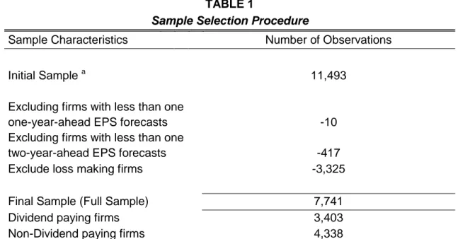
The initial sample contains data for U.S. non-financial firms with publicly traded stock, with the fiscal year end in December, followed by at least one analyst and with a share price of at least $1. Imposing on this sample the additional request for at least one one-year and one two-year-ahead EPS forecasts and positive net income figures the sample reduces its observations from 11,493 to 7,741. These additional requests are necessary to guarantee the existence of relevant data for further analysis. Selecting only positive net income observations makes the usage of the P/E multiple a viable option. Within this sample 4,338 observations belong to non-dividend paying firms, while 3,403 observations belong to dividend paying firms (table 1).
25 TABLE 1
Sample Selection Procedure
Sample Characteristics Number of Observations
Initial Sample a 11,493
Excluding firms with less than one
one-year-ahead EPS forecasts -10
Excluding firms with less than one
two-year-ahead EPS forecasts -417
Exclude loss making firms -3,325
Final Sample (Full Sample) 7,741
Dividend paying firms 3,403
Non-Dividend paying firms 4,338
a
The Initial Sample already requires a December fiscal year end, excludes financial firms and imposes the share price to be higher than $1.
Table 2 shows the sub-sample characteristics in terms of industry, profitability and size. Note that dividend and non-dividend paying firms are present in mostly the same industries. Profitability and size differ, however, considerably across both sub-samples.
TABLE 2
Sample Characteristics
Type Industry Compatibility Profitability Size
Dividend Paying 0.999 696.820 3,906.135
Non-Dividend Paying 0.992 122.171 836.023
Industry presence across sub-samples. Profitability and size are measured in millions.
When performing the analysis on the P/E multiple, the median two-year-ahead EPS forecast provided by I/B/E/S is the chosen value driver. This selection relies on the superior performance of this value driver compared to the one-year-ahead EPS forecast and the actual earnings, both provided by I/B/E/S, as well as the two EPS values provided by Compustat adjusted for stock splits. The second multiple-based analysis is the price to book multiple. This analysis incorporates the value driver from the Compustat data, once it is an accounting value. Common/Ordinary Equity is divided by Common Shares Outstanding, which are than adjusted for stock splits.
26 In both cases the multiples are calculated through the industry harmonic mean as this method diminishes the effect of extreme values, reporting less biased estimates. A more sophisticated method presented by Bhojraj and Lee (2002) is neglected as the practicality of the multiple based methods relies on its simplicity.
The first flow-based model presented is the RIVM. This model is estimated with a forecast period of two years, according to the Edwards-Bell-Ohlson-type approach, coined by Bernard (1994) as stated by Frankel and Lee (1998). The intrinsic value is therefore calculated by summing the book value per share at time zero, the residual income for period one and two and finally the terminal value as a growing perpetuity of two-year-ahead residual income.
The second flow based model is the OJM. This model is also estimated with a forecast period of two years. Each firms’ intrinsic value is here calculated by summing the next years’ capitalized earnings per share, the capitalized one-year-ahead and two-one-year-ahead abnormal earnings growth. At last, the terminal value is added as a growing perpetuity of the two-year-ahead abnormal earnings growth.
For both flow based models, the growth rate is initially retained at a conservative level of 0%. The cost of equity is estimated using the following industry cost of equity model:
Where:
After testing long and short term risk free rates along with firm specific and industry specific betas, the short term risk free rate and the industry specific betas show the best results. Consequently, the cost of equity is calculated by
27 summing the 3-month Treasury bill rate and the industry specific beta times the market risk premium which is assumed to be 5%.
If at a later stage the growth rate happens to exceed a firm’s cost of equity the model assumes a zero growth rate preventing a negative denominator. Additionally, if the terminal value assumes negative values, the models replace the terminal value by zero. This is done to avoid negative valuation estimates which would inevitably appear by growing a negative perpetuity. It is hence assumed that if a firm has a negative residual income or a negative abnormal earnings growth for period two it will shortly go out of business.
Note that for each of the four models the respective data is trimmed by fiscal year for relevant variables to eliminate existing outliers which could influence the further analysis of each model.
4.5 Empirical Results 4.5.1 Descriptive Statistics
This analysis follows the work of Francis et al. (2000) using market prices as a benchmark, once using the tracking ability of price variations surpasses the scope of this analysis. The four models are tested in terms of their bias and accuracy, also known as signed prediction errors and absolute prediction errors, where the valuation estimate is set against the actual price.
28 TABLE 3
Descriptive Statistics - Valuation Errors
Panel A: Full Sample Model Mean Median SD P1 Q1 Q3 P99 Signed Prediction Errors a V(P/E) 0.006 -0.052 0.393 -0.665 -0.238 0.168 1.381 V(P/B) -0.019 -0.156 0.622 -0.827 -0.431 0.226 2.262 V(RIV) -0.284 -0.338 0.301 -0.731 -0.474 -0.169 0.775
V(OJ) 0.067 -0.047 0.492 -0.593 -0.243 0.241 1.925
Absolute Prediction Errors b V(P/E) 0.279 0.213 0.276 0.004 0.097 0.372 1.38
V(P/B) 0.453 0.365 0.426 0.014 0.181 0.595 2.262
V(RIV) 0.362 0.354 0.199 0.019 0.222 0.489 0.784
V(OJ) 0.334 0.242 0.367 0.009 0.118 0.415 1.925
Panel B: Dividend Paying Model Mean Median SD P1 Q1 Q3 P99 Signed Prediction Errors a V(P/E) 0.000 -0.046 0.331 -0.600 -0.201 0.141 1.248 V(P/B) -0.066 -0.180 0.586 -0.824 -0.445 0.147 2.163 V(RIV) -0.271 -0.322 0.266 -0.674 -0.435 -0.178 0.693
V(OJ) 0.061 -0.037 0.450 -0.581 -0.214 0.219 1.764
Absolute Prediction Errors b V(P/E) 0.234 0.178 0.234 0.003 0.080 0.310 1.248
V(P/B) 0.427 0.349 0.407 0.013 0.164 0.565 2.163
V(RIV) 0.336 0.334 0.177 0.021 0.213 0.445 0.748
V(OJ) 0.301 0.216 0.341 0.008 0.107 0.376 1.764
Panel C: Non-Dividend Paying Model Mean Median SD P1 Q1 Q3 P99 Signed Prediction Errors a V(P/E) 0.011 -0.060 0.436 -0.682 -0.275 0.205 1.439
V(P/B) 0.017 -0.135 0.646 -0.829 -0.423 0.301 2.304
V(RIV) -0.295 -0.361 0.325 -0.747 -0.509 -0.156 0.874
V(OJ) 0.072 -0.056 0.525 -0.601 -0.268 0.260 2.098
Absolute Prediction Errors b V(P/E) 0.316 0.244 0.301 0.005 0.117 0.417 1.439
V(P/B) 0.474 0.383 0.441 0.014 0.193 0.619 2.304
V(RIV) 0.384 0.381 0.212 0.019 0.233 0.526 0.874
V(OJ) 0.362 0.266 0.386 0.009 0.131 0.454 2.098
a
Bias = (Vj-Pj)/Pj , b Accuracy = |Vj-Pj|/Pj, SD stands for Standard Deviation, P1 for 1st Percentile, Q1 for lower Quartile, Q3 for Upper Quartile and P99 for 99th Percentile.
Panel A of table 3 reports the signed and absolute prediction errors of the full sample for the models under analysis, while panel B focuses on the dividend paying firms and panel C addresses the non-paying dividend firms within the same sample. For each panel and model the mean, median, standard deviation, percentiles and quartiles are presented. The difference between the mean and
29 the median are existing outliers which can influence the mean heavily. As shown the results do not deviate much from each other but given their characteristics the median is a more stable indicator. The other measures indicate the discrepancy within each model and show that the dispersion is normal.
It is important to point out that over the three panels the median signed prediction errors is constantly negative meaning that the valuation estimates are lower than the actual price. This result can be explained by fact that these valuation methods capture the value only through accounting figures, leaving other factors aside and are therefore expected to predict a lower valuation estimate than the actual price.
Over the three panels it is possible to identify the lowest absolute valuation errors in P/E multiple, followed by the OJM, the RIVM and finally the P/B ratio. Also, the valuation errors perform better for dividend paying firm than for non-dividend paying firms. Finally, the better the overall performance of the model, the higher the absolute prediction errors discrepancy between dividend and non-dividend paying firms.
4.5.2 Significance Level Tests
Table 4 builds on the descriptive statistics presented before and tests the signed and absolute prediction errors for each model within and between sample partitions. First, as the median shows to be a more stable indicator (Damodaran, 2002) the Wilcoxon test is applied to test the difference in median within each model between dividend paying firms and non-dividend paying firms. This procedure is applied for both, signed prediction errors and absolute prediction errors. At last, the models are compared against each other. Here also, the Wilcoxon test is applied comparing the median of each model against the others. In all cases tested, the significant difference is enough to reject the null hypothesis claiming the same sample median. Consequently, it is possible to say that within each model as well as between the models the difference is significant.
30 TABLE 4
Comparison of Bias/Accuracy Prediction Errors between/within Sample Partitions
Panel A: Signed Prediction Errors (Bias) a
Model Median % Difference α-Level Difference = 0 V(P/E) -0.052 0.000 V(P/B) -0.156 0.000 V(RIV) -0.338 0.000 V(OJ) -0.047 0.000
Panel B: Absolute Prediction Errors (Accuracy) b
Model Median % Difference α-Level Difference = 0 versus V(P/B) versus V(RIV) versus V(OJ) V(P/E) 0.213 0.000 0.000 0.000 0.000 V(P/B) 0.365 0.000 0.000 0.000 V(RIV) 0.354 0.000 0.000 V(OJ) 0.242 0.000 a
Panel A reports median signed prediction errors, equal to (Vj-Pj)/Pj. It also reports the significance level associated with the Wilcoxon test of whether the median prediction within the models errors are equal to zero.
b
Panel B shows the median absolute prediction errors, |Vj-Pj|/Pj. The last three columns report the significance levels for the Wilcoxon tests comparing the median absolute prediction errors between models. The median values are from the full sample.
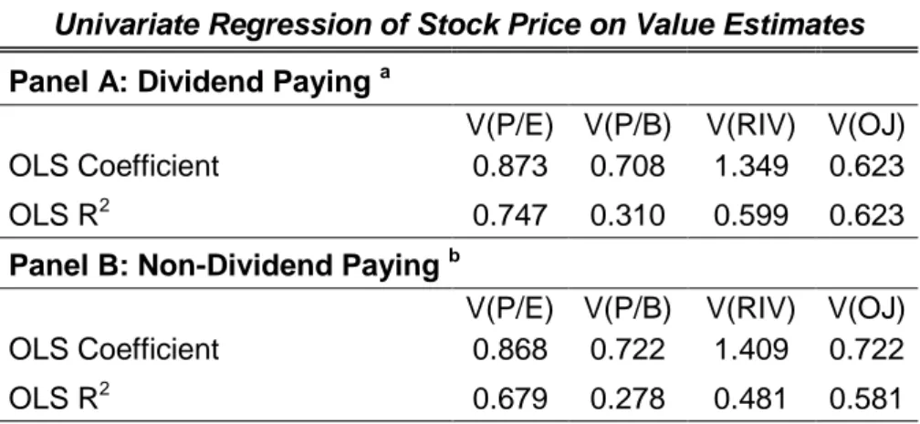
4.5.3 Univariate Regression
This analysis also examines the explainability of each model. Univariate regressions are used to measure the explainability (R2) of stock prices on value estimates. Panel A of table 5 reports the R2 OLS and the OLS coefficient for market prices on the 15th of April on each value estimate for dividend paying firms, while panel B focuses on non-dividend paying firms. In general the variability of the univariate regression ranges from 75% to 28%, and in particular from 75% to 31% and 68% to 28%, for dividend and non-dividend paying firms respectively. This builds on the previous presented valuation errors which were lower for dividend paying firms and performed particularly well for the P/E valuation model. Hence, in both panels the P/E valuation has the highest R2 followed by the OJM, the RIVM and finally the P/B model. Also between both panels the dividend paying firms have a general higher R2 than the non-dividend paying firms.
31 TABLE 5
Univariate Regression of Stock Price on Value Estimates
Panel A: Dividend Paying a V(P/E) V(P/B) V(RIV) V(OJ) OLS Coefficient 0.873 0.708 1.349 0.623
OLS R2 0.747 0.310 0.599 0.623
Panel B: Non-Dividend Paying b V(P/E) V(P/B) V(RIV) V(OJ) OLS Coefficient 0.868 0.722 1.409 0.722
OLS R2 0.679 0.278 0.481 0.581
a Panel A reports results of estimating the following regression: Pj,F=λ0 +
λ1VFj+εj, where Pj,F=observed share price of Dividend Paying Firms j; VFj= Value for security j for the respective models. b Panel B reports results of estimating the following regression: Pj,F=λ0 + λ1VFj+εj, where Pj,F=observed share price of Non-Dividend Paying Firms j; VFj= Value for security j for the respective models.
4.5.4 Robustness Test
Many studies, like Francis et al. (2000), perform robustness tests to growth rates since this assumption influences the empirical outcome considerably. The growth rate impacts only two models, the RIVM and the OJM. Having set the growth rate at the beginning at a conservative level of 0% the growth rate will now be increased to 2%.
Table 6.1 compares the signed and absolute prediction errors for dividend paying firms and non-dividend paying firms. Across panels, the RIVM and the OJM show a slight improvement within absolute prediction errors, following the results shown by Francis et al. (2000) in which the prediction errors diminished with a higher growth rate. The OJM shows, however, positive signed prediction errors. This means that with an increasing growth rate the OJM predicts valuation estimates which exceed the actual price making the signed prediction errors positive.
32 TABLE 6.1
Robustness Test
Descriptive Statistics
Panel A: Dividend Paying Growth rate = 0% Growth rate = 2% Signed Prediction Errors a Model Mean Median Mean Median
V(RIV) -0.271 -0.322 -0.242 -0.327 V(OJ) 0.061 -0.037 0.128 0.043 Absolute Prediction Errors b Model Mean Median Mean Median
V(RIV) 0.336 0.334 0.312 0.303 V(OJ) 0.301 0.216 0.302 0.213 Panel B: Non Dividend Paying Growth rate = 0% Growth rate = 2% Signed Prediction Errors a Model Mean Median Mean Median
V(RIV) -0.295 -0.361 -0.247 -0.327 V(OJ) 0.072 -0.056 0.149 0.037 Absolute Prediction Errors b Model Mean Median Mean Median
V(RIV) 0.384 0.381 0.373 0.363
V(OJ) 0.362 0.266 0.368 0.253
a
Bias = (Vj-Pj)/Pj , b Accuracy = |Vj-Pj|/Pj.
In table 6.2 the analysis shows that even though the absolute prediction errors decreased with an increasing growth rate, the sub-samples are still significantly different from each other to reject the null hypothesis of the medians within the sample are equal.
TABLE 6.2
Robustness Test - continued
Comparison of Bias/Accuracy Prediction Errors within Sample Partitions Panel A: Signed Prediction Errors (Bias) a
Growth rate Model Median % Difference α-Level Difference = 0
0% V(RIV) -0.338 0.000
0% V(OJ) -0.047 0.000
2% V(RIV) -0.308 0.000
2% V(OJ) 0.041 0.000
Panel B: Absolute Prediction Errors (Accuracy) b
Growth rate Model Median % Difference α-Level Difference = 0
0% V(RIV) 0.354 0.000
0% V(OJ) 0.242 0.000
2% V(RIV) 0.332 0.000
2% V(OJ) 0.256 0.000
a
Panel A reports median signed prediction errors, equal to (Vj-Pj)/Pj. It also reports the significance level associated with the Wilcoxon test of whether the median prediction within the models errors are equal to zero. b Panel B shows the median absolute prediction errors, |Vj-Pj|/Pj and its associated significance level. Both panels show results for two growth rates 0% and 2%.