Equity Valuation : Arezzo&Co

(1)

September, 2014

Arezzo&Co Equity Valuation

Arezzo&Co is a Brazilian company, among the leaders in the women footwear retail market in Latin America. It designs and develops affordable luxury shoes and accessories under the brand names Arezzo, Schutz, Anacapri and Alexandre Birman.

The company operates a very flexible business model, in which all shoes and accessories are designed internally, but its production can be either handled internally or outsourced to third-party manufacturers. Similarly, its sales strategy is based on a combination of owned, franchised and multi-brand stores, as well as a recently developed e-commerce platform. This flexible business model allows the company to determine the most profitable combination of the above factors, without losing control over its brands, product design and quality, while generating high returns on invested capital.

Arezzo&Co benefits from Brazil’s dynamic consumption market, in which branded products assume a greater importance as Brazilians move up the income ladder. Despite the recent economic slowdown, the prospects for the domestic retail sector remain strong.

Based on a 5-year DCF valuation, it is estimated a price target of R$ 30.0 per share for Arezzo&Co. At current values, this price target implies a 6.1% upside, which results in a HOLD recommendation.

SEPTE MBE R, 2014

Inês de Carvalho Frei re

152210008

Jos é Carlos Tudel a Martins

Advi sor

DISCL AIMER

Diss ertation submitt ed in

parti al ful fillm ent of

requi rements for t he degree

of MSc in Economics, at

Universidade Cat óli ca

Portuguesa

S h a r e p r i c e a s o f J u n e , 2 0 1 4 S o u r c e : B l o o mb e r g Arezzo&Co HOLD 6.1% upside TARGET PRICE Bloomberg Ticker Share Price Market Cap R$ 30.0 ARZZ3 R$ 28.3 R$ 2,508M

(2)

Equity Valuation

Arezzo&Co

Inês de Carvalho Freire

152210008

Advisor: José Carlos Tudela Martins

Dissertation submitted in partial fulfillment of requirements for the degree of MSc in Economics, at

the Universidade Católica Portuguesa

(3)

ABSTRACT

Arezzo&Co is a Brazilian company, among the leaders in the women footwear retail market in Latin America. It designs and develops affordable luxury shoes and accessories under the brand names Arezzo, Schutz, Anacapri and Alexandre Birman.

The company operates a very flexible business model, in which all shoes and accessories are designed internally, but its production can be either handled internally or outsourced to third-party manufacturers. Similarly, its sales strategy is based on a combination of owned, franchised and multi-brand stores, as well as a recently developed e-commerce platform. This flexible business model allows the company to determine the most profitable combination of the above factors, without losing control over its brands, product design and quality, while generating high returns on invested capital.

Arezzo&Co benefits from Brazil’s dynamic consumption market, in which branded products assume a greater importance as Brazilians move up the income ladder. Despite the recent economic slowdown, the prospects for the domestic retail sector remain strong.

Based on a 5-year DCF valuation, it is estimated a price target of R$ 30.0 per share for Arezzo&Co. At current values, this price target implies a 6.1% upside, which results in a HOLD recommendation.

(4)

PREFACE

The conclusion of this dissertation is not only the so expected end of my master’s degree but also the proof that with hard work, persistence and, above all, the support of an amazing family and friends everything is possible.

First, there are no words available in the world to express the gratitude I have for the unconditional love, patience and support of my parents, Graça Galvão and Francisco Freire. Between two continents, three countries and thousands of late hours on the phone, they were always available to help me, listen and to give me strength towards the conclusion of this work.

Second, I would like to thank all my professors at Católica-Lisbon, especially my advisor prof. Tudela Martins for his constant availability and quick response to all my questions and doubts, as well as to Arezzo&Co investor relations’ Leonardo Reis and Vanessa de Oliveira for their contribution to this work.

Last but not the least, I want to thank all my friends and colleagues, spread between Portugal and Brazil, for their amazing friendship and ability to keep me smiling during the entire process of this dissertation. I would specially thank G8, the best combine classmates and friends I will ever have, my lifetime friends that prove that there is no distance, nor years, that can offset our companionship, and all my friends at Católica-Lisbon, especially Francisca Horta for her patience and helpful feedback.

To everyone that supported me during this dissertation and not mentioned above, a big thank you.

(5)

1. INTRODUCTION

The aim of this dissertation is to present a fair valuation of Arezzo&Co’ shares based on a complete and thorough analysis of its business model and future prospects as well as on a detailed study of the various valuation methodologies commonly used by equity research analysts.

Arezzo&Co is a Brazilian company among the leaders in the footwear and accessories industry in Brazil. It designs and develops women shoes and accessories under four brand names: Arezzo, Schutz, Anacapri and Alexandre Birman. The company has an interesting asset light business model that combines both own and outsourced production as well as several different sale channels, from owned and franchised stores to multi-brand retailers and an e-commerce platform. The reason for choosing this company has to do with its interesting and complementing business model and with the fact that it operates in an industry with good future prospects in Brazil and significant tradition in Portugal. Being the Portuguese shoes a reference for its quality and having Arezzo&Co no relevant presence in Europe, presenting Arezzo&Co in this dissertation could inspire further studies on the company’s future strategy, that could consist of a potential internationalization of its manufacturing facilities to Portugal as a way to penetrate and compete within the European footwear market.

Throughout the years, the issue of companies’ valuation has been subject of discussion among finance practitioners and, until the moment, there is no “one sizes fits all” approach for every company. Therefore, in this dissertation a brief overview of the most commonly accepted valuation methodologies, its main characteristics, advantages and disadvantages will be presented firstly. Secondly, and in order to start analyzing the company’s business model, the recent major macroeconomic developments in Brazil as well as the most relevant aspects of the footwear and accessories industry in the country are presented. Based on the industry momentum, on Arezzo&Co business model and growth perspectives the DCF valuation methodology is chosen as the most suitable method in this case. However, since there is no single correct answer to value a company, a sensitivity analysis to the most relevant operational and valuation parameters that influence the company’s DCF valuation is also presented as well as a Relative Valuation in order to complement and to ensure that growth assumptions are in line with what the market believes to be correct.

To conclude, the results of this dissertation are compared to those of a selected equity research analyst, with the aim of highlighting and justifying the main differences encountered.

(7)

2. LITERATURE REVIEW

2.1 VALUATION METHODS

The issue of Companies Valuation has been subject of discussion in Finance for several years, thus there is a broad range of different opinions and ideas on the topic. According to Damodaran (2002) there are three main consensual methods for valuing firms: the discounted cash flow (DCF) models, the relative valuation (method of multiples) and the real options valuation (option pricing models). All of them share common characteristics and can be seen almost as a simple rearrangement of the same methodology, with the only differences being the underlying assumptions (Young et al., 1999). This well shared idea has real practical relevance since it gives the opportunity for finance practitioners to compare different valuation estimates arising from different valuation approaches with the ability to understand what were the assumptions causing this difference (Young et al., 1999). The following sections will go into detail on the first two methods outlined by Damodaran, leaving the option pricing valuation apart since it will not be used in the case study in question.

2.1.1 DCF models

The foundations of the DCF valuation method is based on the present value approach and on the valuation findings of Professors Merton Miller and Franco Modigliani (1958).

The idea behind this method is that the value of an asset is simply the future cash flows generated by that asset, discounted to the present at a rate reflecting the riskiness associated with those cash flows and added up at the end (Luehrman, 1997a). However, when valuing firms, the consensual approach is to estimate its cash flows for a specific explicit period and after that time assuming a steady state condition for the firm. At this steady state condition, one should consider a terminal value for the cash flows that grow at a constant nominal rate in perpetuity (Kaplan and Ruback, 1996).

𝑉𝑎𝑙𝑢𝑒 = ∑ 𝐸[𝐶𝐹𝑡] (1 + 𝑟)𝑡 𝑛 𝑡=1 +𝑇𝑒𝑟𝑚𝑖𝑛𝑎𝑙 𝑉𝑎𝑙𝑢𝑒𝑛 (1 + 𝑟)𝑛 Where,

E[CFt] – Estimated Cash Flows in period t

r – Discount Rate

(8)

Since it becomes difficult to accurately forecast cash flows after the explicit period considered, it is assumed that cash flows stabilize and the Terminal Value can be calculated. The terminal value is an important piece of a DCF valuation since it often represents a large portion of the total value of the firm (Hitchner, J., 2003). By assuming that the firm will continue on growing at a constant rate forever, the terminal value can be estimated as follows:

𝑇𝑒𝑟𝑚𝑖𝑛𝑎𝑙 𝑉𝑎𝑙𝑢𝑒_𝑛 =𝐸[𝐶𝐹𝑛+1]

𝑟−𝑔

Where,

E[CFn+1] – Estimated Cash Flows one year after the Explicit Period

r – Discount Rate

g – Constant Growth Rate

As a firm grows and time passes, the firm will eventually start growing at less than or equal to the nominal growth rate of the economy, reflecting both the expected inflation and real growth rates (Kaplan and Ruback, 1996).

2.1.1.1 Cash Flows Definition

There are several ways of applying this valuation approach. One can opt to value a firm as a whole, using Free Cash Flow to the Firm (FCFF1_{) as input to the model, or to value the firm}

directly to equity holders, using Free Cash Flow to Equity (FCFE2_{) instead. While FCFF}

reflects the cash flows generated by the firm’s operation activity that are available for all the capital providers, the FCFE reflects only those cash flows available for the equity owners (Copeland, Koller and Murrin, 2000). This distinction implies two different techniques of the same valuation method: the enterprise DCF model and the equity DCF model (ECF), respectively. These two approaches use different cash flows and discount rates. However they will yield consistent estimates of the firm value as long as there are no mismatch between cash flows and discount rates.

2.1.1.2 Discount Rate Estimation

In finance, risk is defined as the possibility of actual returns differing (for better or worse) from

1_{FCFF – The residual cash flow after meeting all operating expenses, reinvestment needs and taxes but prior to any payments}

to either debt or equity holders. (Damodaran, 2002)

2_{FCFE – The residual cash flow after meeting all expenses, reinvestment needs, tax obligations and net debt payments.}

(9)

the expected returns projected by investors. Since risk cannot be observed directly, finance analysts have developed several ways of estimating it, using available market data, usually past data when considered representative of investors’ future expectations. This gives rise to the most controversial piece of a DCF valuation: the discount rate. This rate is seen as the opportunity cost of capital, that is, the return an investor expects to earn by investing his money in a similar project with similar risk as the one of the cash flows being discounted (Luehrman, 1997b).

Therefore, the discount rate also referred as the cost of capital works as a mirror of the risk inherent to the cash flows. It depends on who is providing the capital, i.e., it depends if we are talking about equity investors, debt capital providers or both.

2.1.1.2.1 Cost of Debt

The cost of debt is the current rate a company pays on interest-bearing debt securities, assuming that the firm is borrowing at market rates (Hitchner, J., 2003).

The simplest case for computing the cost of debt is when a company has long term bonds being widely traded on the market. In these situations, the cost of debt can be considered as the yield subjacent to these long-term bonds. However, when this is not the case, Damodaran (2002) claims that the cost of debt can be roughly estimated by adding a risk-free rate and the default spread of the company.

k_d= r_f+ default spread

The discussion on the choice of the risk free rate will be addressed in the next section while assessing the issue of estimating the cost of equity. The default spread is the compensation for the risk of a company not being able to honor its debts. Once debt is always senior to equity the only reason for a company to default on its payment is not having sufficient cash flows to cover it. Usually, firms are rated by rating agencies (such as Moodys or S&P) and consequently have an associated default spread, which can be used to compute the cost of debt. When this is not the case, an analyst may construct a synthetic default spread based on interest coverage ratios3

(Damodaran, 2002).

(10)

2.1.1.2.2 Cost of Equity

In opposite to the cost of debt, the cost of equity is much more difficult to compute since we cannot directly observe it in the market. The most commonly model used to estimate its value is based on the Capital Asset Pricing Model and is referred to as CAPM. However, there are several other estimation models, such as the APM4_{and the Multifactor models that highlight}

other key risk factors different from what CAPM considers.

I. CAPM (1964)

Sharpe5_{was the first to introduce the CAPM. The underlying assumption of the model is that}

equity investors are well diversified, i.e. they are only faced with undiversifiable risk – the Market Risk.

According to CAPM, the cost of equity (ke) is assumed to be equal to the sum of the return

provided by a risk-free asset and a risk premium that compensates the investor’s exposure to the Market Risk, which in turn is adjusted by the parameter β (systematic risk) that represents the security’s sensitivity to the market. The translating equation of the model is the following:

𝑘𝑒= 𝑟𝑓+ 𝛽[𝐸(𝑟𝑚) − 𝑟𝑓]

Where,

𝑟𝑓 – Risk-free rate

𝛽 – Systematic risk (beta)

[𝐸(𝑟_𝑚) − 𝑟_𝑓] – Market risk premium

To carry on with the computation of the ke through CAPM, it is necessary to estimate each one

of the three elements that compose the equation: the risk-free rate, the market risk premium and the β.

Risk-free rate

In theory, the risk-free rate is the return required by investors on a default-free security or portfolio of securities. Therefore, the best estimate for this risk-free asset would be the return on a zero-beta portfolio of securities, constructed in a way that produces the minimum variance possible. However, due to complexity problems associated with the computation of such

4_{Arbitrage Pricing Model}

(11)

portfolio, Copeland, T. et al. (2000) suggest that the best proxy for the risk-free rate is a 10-year government bond. The reason behind such assumption is the fact that usually this bond matches both the duration of the cash flows of the firm being valued and the stock market index portfolio considered. This provides consistency to the valuation, the β and the market-risk premium. Additionally, it is also important to stress that 10-year government bond is normally less sensitive to changes in inflation and has relatively low liquidity premium in comparison to longer-maturity government bonds.

Market Risk Premium

The market risk premium, or equity risk premium (“ERP”), used in CAPM is the average return demanded by investors as a premium over the risk-free rate for investing in an equity portfolio diversified both within and across sectors. Among practitioners, historically, this well diversified portfolio has been considered the local market index. However, this assumption should be revised when one is considering countries with relatively small and risky listed companies. The same revision applies when estimating the market risk premium for non-mature economies. Damodaran (2002) recommends the use of the market risk premium from a mature market, like the United States, plus a country risk premium adjustment, based either on default risk spreads, on relative standard deviations or both.

The estimation of the market risk premium is often made by looking at historical values (Damodaran 2010), assuming that some period of the past provides the best indication of the future. Ibbotson Associates produces an annual publication called “Stocks, Bonds, Bills and Inflation” (“SBBI”) that provides one of the most commonly cited equity risk premium estimates in the field of valuation. The equity risk premium is calculated by Ibbotson Associates using the average return on the S&P500 over the average return on default-free securities and compiles data from 1926 until the present time.

There are three main controversial issues when choosing the right ERP: the risk-free security, the horizon period and the averaging technique considered. According to Damodaran (2010), “the risk free rate chosen in computing the risk premium has to be consistent with the risk free rate used to compute the expected returns”. Thus, if the 10-year government bond is used in CAPM as the risk free rate, the ERP has to be the premium earned by stocks over that rate. Regarding the time period considered, some practitioners argue that risk aversion of investors is likely to change over time and therefore using a shorter period provides a more accurate estimate. On the other hand, considering shorter-periods brings noise to the valuation (increasing the standard errors) and consequently overwhelming the advantages of more

(12)

updated information. Additionally, even the most recent periods contain unique events that may induce investor’s risk aversion. Thus, by including market data measured over the entire set of economic scenarios available, the model can better anticipate similar events in the future instead of overemphasizing one period over another (Annin and Falaschetti, 1998). To conclude, in what concerns the averaging technique applied, the arithmetic average is more consistent with the mean-variance framework of CAPM and thus, apparently, a better predictor for the risk premium. However, geometric average takes compounding into account and is therefore a better predictor in the long run. For valuation purposes where there is the need to discount cash flows over a long period of time the most accurate measure would then be the geometric average.

Finally, as it was previously stated, countries with relatively short and volatile equity markets histories should add an extra variable to its equity premium, which is referred in literature as the country risk premium. There are several measures of country risk and one of the easiest and most accessible is the rating assigned to a country’s debt by rating agencies (S&P and Moody’s, for example). This rating reflects the default risk of the country, which is, in many ways, affected by the same factors that drive the equity risk and is associated with a default risk spread over the US treasury bonds (Damodaran, 2010). However, this is only a measure of the country’s default risk and thus one would expect the country equity risk premium to be larger than the default risk spread. Damodaran (2010) suggests looking at the volatility of the equity market in the country relative to the volatility of the country bond to estimate the additional spread. On the other hand, there are other numerical country risk scores that have been developed by entities and services that represent a much more comprehensive measure of a country’s risk. In Brazil, the most commonly used measure is the Emerging Markets Bond Index – Brazil (“EMBI+Brazil”) and it was developed by J.P. Morgan Chase. According to the Brazilian Central Bank, this measure reflects the weighted average premium paid by a portfolio of Brazilian external debt securities denominated in US dollars over the treasury bonds of the United States. It is important to note that this measure is in US dollars and therefore it is necessary to add a currency exchange rate adjustment to bring this figure to the national currency, Brazilian Real. A simple way is to add the difference between the long-term inflation rates of the United States and Brazil, since in the end the purchasing power parity should remain the same.

Beta (β)

In order to capture the systematic risk, the equity risk premium (market risk) is adjusted by the beta (β) – a measurement of volatility of the excess return of an individual security relative to that of the market portfolio (Hitchner, J., 2003). Each public company has a correspondent beta

(13)

and the stock market as a whole has a beta equal to 1. Therefore, this measure can be interpreted the following way:

β > 1 => the security is riskier than the market; β < 1 => the security is less risky than the market.

In finance, there are several opinions on how to better estimate the beta for a company. Yet, the most conventional one is to estimate it by regressing the historical returns of the firm against the historical returns of the market index. When doing this regression, an analyst has three major choice concerns to take into account: the length of the estimation period, the return interval and the market index that should be considered. The task of choosing such parameters is relatively more important when the markets have few stocks listed or are dominated by one or few major stocks. Besides, from this approach result betas that are almost always too noisy or skewed due to the several estimation assumptions required. Thus, this method is not considered as the most useful measure of a company’s equity risk. Moreover, this approach is not possible for private firms, or for those whose stocks have not been traded in the market for a long period. As a solution, some authors argue that estimating an industry average beta is better. The industry average beta is typically more stable and reliable than an individual company beta since measurement errors tend to cancel out (Copeland, et al, 2000). To construct this beta, it is necessary to find the betas of comparable listed companies unleveraging them and then compute the average. The unleveraging process is necessary since each beta found (called levered beta) reflects the capital structure of the associated company. The final beta to use in the valuation procedure is then the average industry beta adjusted for the capital structure of the specific company being valued. It can be done by applying the following formula (Damodaran, 2002):

𝛽𝑙 = 𝛽𝑢[1 + (1 − 𝑡)

D E]

Where,

βl – Company’s Beta (levered beta)

βu – Industry Average Beta (unlevered beta)

t – Tax rate

D/E – Debt to Equity Ratio

Given that the beta is regarded as the tendency of a security’s return to respond to fluctuations in the market, it is common understanding that cyclical firms (operating in businesses more sensitive to market conditions) will have higher betas. Moreover, an increase in financial

(14)

leverage (D/E) will increase the variance in the net income of the company, making the equity investment in the firm much riskier. The same can be concluded for operating leverage decisions.

It is also important to note that the beta for a firm is a weighted average of the betas of all the different businesses the firm operates in using as weight the proportion of the firm’s value resultant from each business.

As it was previously said, there are other models that also estimate the cost of equity of a security. These models relax some of the restrictive assumptions that CAPM imposes such as ignoring transaction costs or the supposition that investors do not have access to private information.

II. APT and Multifactor Models

The Arbitrage Pricing Model (APM) appears as a more generalized version of the CAPM with the only restriction being that securities faced with the same exposure to the market have to be traded at the same price. The rationale behind the estimation of the cost of equity (ke) is similar

to that of the CAPM, however instead of considering only the market portfolio risk it allows for unspecified market risk factors to be accounted for in the model arguing that the beta from the market risk premium does not fully explain the systematic risk (Damodaran, 2002). The fact that APM does not specify the risk factors to take into consideration leads to the appearance of other models. Several authors suggest specific economic variables for the undefined statistical factors. For example Chen, Roll and Ross (1986) suggest that industrial production, changes in default premium, shifts in the term structure, unanticipated inflation and changes in the real rate of return are variables that can be used to come up with a model for estimating the ke. Others like Fama and French (1993) suggest a three-factor model, where the factors are not

only the risk premium on the market portfolio but also the risk premiums on small size and high book-to-market ratio firms, respectively.

(15)

2.1.1.3 Main DCF Approaches

2.1.1.3.1 WACC Based Approach

Historically the standard approach to a DCF valuation has been to discount the FCFF at the weighted average cost of capital (WACC). The reasoning for assuming this rate is that it should reflect the cost of each source of capital weighted by the value they have on the capital structure of the firm, this way capturing all the value created or destroyed by the firm’s financing program. In this approach the tax benefits of having debt in a company’s capital structure are taken into account within the WACC formula. In Brazil, this tax benefits consider both the income tax (IR) and the social contribution on net income (CSLL). The cost of debt and the cost of equity are both estimated as it was described in previous sections.

WACC = k_e E D + E+ kd D D + E(1 − t) Where, ke – Cost of Equity

kd – Cost of pre-tax Debt

t – Current tax rate for the company D – Pre-tax debt, in market values E – Equity, in market values

The correct approach to the WACC-based DCF valuation is to consider a different WACC for each year reflecting the capital structure of that year. However, given that this would demand several computations, Copeland et al. (2000) suggest that the same WACC should be used in all the projection period. Moreover, they suggest that one should think about a target capital structure rather than the current structure of the firm since changes like management financing decisions or changes in the market value of the outstanding securities may occur in a way that the current capital structure does not reflect the capital structure prevailing over the whole period. There are three steps to follow in order to find the target capital structure:

- Estimate the current market value based capital structure of the firm - Review the capital structure of comparable firms

- Review management choices for financing the business and its implications

However, Luerhman (1997a) states that the WACC-based method is currently considered obsolete. It does not mean that this methodology no longer works but instead, advances in

(16)

technology and software as well as valuation models more tailor-made according to manager’s needs are now considered superior to this old fashion method.

2.1.1.3.2 APV Approach

“To divide and conquer” (Brealey, 2008)

Nowadays a better alternative valuation methodology is to value each business operation independently and then add-up their respective present values. This approach is called Adjusted Present Value (APV) and relies on the idea of value additivity. It allows managers to realize the main sources of value creation within the firm and to configure the valuation in the way that makes more sense for the people managing each segment (Luerhman, 1997a).

The first step in using this method is to estimate the present value of the firm (Vu) as if it was

entirely financed with equity, i.e., considering that it has no debt. For this purpose, one should discount the after-tax FCFF using the opportunity cost of capital that, in this case, is simply the unleveraged cost of equity, i.e., the ke computed using the unleveraged beta (βu) of the firm.

Second, the financing side effects should be taken in consideration and the present value of its costs and benefits to the firm have to be calculated. The largest side effects of a company’s financing program are the interest tax shield on debt (a plus) and the bankruptcy costs (a minus) (Damodaran, 2002). Regarding the computation of the present value of the interest tax shield one should use the following formula:

PVTS = ∑ t × kd× D𝑖 (1 + k_d+ 𝜋_𝑑)𝑖 𝑛 𝑖 + 𝑇𝑒𝑟𝑚𝑖𝑛𝑎𝑙 𝑉𝑎𝑙𝑢𝑒_𝑛6 (1 + k_d+ 𝜋_𝑑)𝑛 Where,

t – Marginal tax rate (assumed constant in perpetuity) kd – Cost of debt

kdxD – Interest on debt

πd – Probability of default

There is some discussion among academics on which rate should be used to discount the interest tax shield. Some agree that interest payments as well as interest tax shield fluctuate for the same reasons as the operating cash flow and therefore should be discounted at the corresponding rate.

6_{𝑇𝑒𝑟𝑚𝑖𝑛𝑎𝑙 𝑉𝑎𝑙𝑢𝑒}

(17)

Others consider the interest payments as risky as the principal and therefore the interest tax shield should be discounted at the cost of debt. However, Luerhman (1997b) concluded kd to

be the best approach if one considers an upward adjustment since in some extreme situations companies may be able to pay the interest on debt but are unable to benefit from its tax shields. This leads one to assume the latter as more risky and therefore deserving a higher discount rate. A common upward adjustment can be simply to add the probability of default to the cost of debt, which can be extracted from bond ratings for the respective type of debt.

Korteweg (2007) estimates the bankruptcy costs in a general way, including the total distress costs both before and after default. He finds that these costs can be identified from the market value and beta of firm’s debt and equity. Korteweg also states that on average these costs are around 26.2% of firm’s value, considering all the industries. Damodaran (2002) suggests that the present value of the bankruptcy costs can be calculated by multiplying the value of the unleveraged firm by the percentage of these costs for each period:

PVBC = ∑ BC

(1 + kd+ 𝜋𝑑)𝑖 𝑛

𝑖

Where,

BC – Bankruptcy Costs as percentage of the unleveraged firm value πd – Probability of default after considering debt

The final enterprise value appears as a sum of each different component of value. Since the PVTS only occurs while the firm is still operating, this component of value must be multiplied by the probability of no default. In turn, the PVBC must be multiplied by the probability of default.

𝐸𝑛𝑡𝑒𝑟𝑝𝑟𝑖𝑠𝑒 𝑉𝑎𝑙𝑢𝑒 = 𝑉𝑢+ (1 − 𝜋𝑑) × 𝑃𝑉𝑇𝑆 − 𝜋𝑑× 𝑃𝑉𝐵𝐶

The fact that APV allows accounting for several financing side effects rather than just only the interest tax shield is one of the reasons why this approach is seen as an upgrade of the WACC method. Moreover, there are several times where WACC is not the appropriate method to use and APV always seems to work in those cases. For instance, WACC is only useful when a company has a very simple and constant capital structure – otherwise one would have to be always adjusting for changes in the firm’s capital structure. Companies with complex tax positions will also be poorly served with WACC.

(18)

To conclude, it is important to stress that the power of APV relies on the managerial relevant information it can provide. Managers are no longer stuck with only the information about how much a company is worth but have also full access to where the value comes from.

2.1.1.4 Applicability and some drawbacks of DCF Valuation

The fact that discounted cash flow valuation relies on the estimation of cash flows to the future and respective discount rates makes this methodology more suitable for some firms than others. Companies where these forecasted cash flows are well founded, and where a proxy for risk can be found and used to obtain the discount rates are for sure more appropriate targets for this kind of technique. According to Damodaran (2002), there are some concerns when doing the DCF valuation, like the measurement of risk of the cash flows for private firms. Most risk/return models usually consider risk parameters from historical market prices of the asset being analyzed, which for a private firm is not possible. Nevertheless, a flexible solution to go around this problem is to look at the riskiness of comparable traded companies.

2.1.2 Relative Valuation

As Goedhart, Koller and Wessels (2005) state, “any analysis is only as accurate as the forecasts it relies on” and thus performing a relative valuation, or Multiples Valuation, appears as a useful tool to complement and enhance a DCF valuation. The objective of such valuation is to value an asset based on how similar assets are priced within the market, relying on the assumption that the market is correct on average (Damodaran, 2002). Furthermore, it works as a tool for companies to understand the differences between their performance and that of its competitors as well as a way to recognize the key factors that create value in the industry.

A multiple is simply the ratio between a market value and a key statistic that is assumed to be related with that market value (Suozzo et al., 2001):

Multiple = Market Value of the Asset Measure of Value of the Asset

This method, also known as Relative Valuation, is a four-step procedure, where the first two steps consist in selecting the relevant value measures and the identification of the set of comparable firms, the peer group (Milicevic, 2009). After gathering all the market value variables and the value driver measures for all the elements of the peer group, it is possible to calculate the multiples for each peer. The third step is to aggregate all these multiples into single

(19)

numbers and estimate synthetic peer group multiples. Finally, to determine the value of the firm being valued, the synthetic peer group multiples must be applied to the corresponding value driver of the firm in question (Milicevic, 2009). The hypothesis of this method allows estimating what the market would currently pay for the firm being valued. However, there is no obvious method to determine which measures of value are the most appropriate ones for constructing the valuation (Kaplan and Ruback, 1996).

For simplification purposes, Suozzo et al. (2011) suggest two major types of multiples: the enterprise multiples and the equity value multiples. The enterprise multiples express the value of the entire firm, i.e., the value of all claims on a business relative to a statistic that relates to the entire firm, such as sales and EBIT. On the other hand, equity value multiples express only the value of shareholder’s claims on the firm, relative to a statistic that applies only to the shareholders, such as earnings (the residual left after payments to all non-equity claimants). Practitioners prefer to use equity value multiples because market capitalization does not require a further adjustment for net debt as it is the case with enterprise value multiples. Additionally, Goedhart, et al. (2005), stress that it is always better to consider forward measures rather than historical ones since they are more accurate predictors of future value and, when that is not possible, one shall consider the latest possible data7_{of the historical period. Therefore, the most}

widely used multiples are based on companies’ earnings (net income), book values or revenues (sales).

According to Damodaran (2012), multiples based on earnings are the most commonly used among analysts and are determined by the same fundamentals that determine the value of a firm in a DCF model: expected growth, risk and cash flow potential8_{. An example of such type is}

the Price Earnings Ratio (P/E)9_{that is simply the market value of equity per share divided by}

the earnings per share. However, this ratio is not flawless since the way in which earnings per share are estimated across firms may vary. Moreover, Goedhart, et al. (2005) state that the P/E ratios have also two more additional drawbacks: they are affected by the capital structure of the firms, which can be manipulated, and the earnings contain several non-operating items, such as on-off time events, that can mislead the valuation.

Similarly to multiples based on earnings, the book value multiples are also influenced by the same determinants as the DCF model. However, one of the most important determinants is the

7_{The last four quarters data, called Trailing multiple.}

8_{Firms with higher growth rates, lower risk and higher payout ratios, with other things remaining equal, should trade at much}

higher multiples of earnings than other firms.

9_{P/E =}Market Price per share

(20)

return on equity (ROE)10_{earned by the firm. The Price-to-Book Ratio}11_{can be computed by}

dividing the total market value of equity by the total book value of equity, where the market value of equity reflects the markets’ expectation in what concerns firm’s earning power and cash flow generation, while the book value of equity is simply the difference between the book value of assets and the book value of liabilities. For Damodaran (2012), the major advantage in relation to the earnings multiples is that firms with negative earnings can be valued using this sort of ratios.

Finally, in the most recent years analysts have increasingly turned to alternative multiples such as multiples of revenues12_{or firm-specific measures. There are significant advantages in using}

measures like revenues since these are always available even for more troubled firms and they are relatively difficult to manipulate as other accounting values such as earnings. However, it can also mislead an analyst to assign a high value for a firm that is generating a lot of revenues while losing significant amounts of money. A company needs both to generate profits and cash flows in order to have value.

To sum up, while performing a valuation based on comparable companies one should be aware of three main issues: all multiples relying on accounting rules may be subject to some type of manipulations; to understand what is considered a typical high or low value for a multiple; and to identify what are the main fundamentals determining the multiple and the implications of its alterations on that same multiple.

2.1.2.1 Applicability and some drawbacks of Multiples Valuation

Relative valuation is particularly useful when there are a large number of comparable firms being traded on the market where the company being valued operates. However, although intuitive and easy to use its qualities are also its main drawbacks. The process of selecting the appropriate set of comparable firms can be very difficult since companies should be similar in several aspects, such as: growth rates, cost of capital, capital structure, ROIC13_{and/or the}

business composition. This choice is also somewhat subjective and can be affected by the selection of the analyst that best suits his/her intuition about the firm. Identifying the sector where the firm operates in or, for example, looking at the main competitors stated in a firm’s Annual Report could be two possible ways of reducing this problem. Another problem is the

10_{Higher (lower) returns lead to higher (lower) price-book ratios.}

11_{Price to Book Ratio =}Market Value of Equity

Book Value of Equity

12_{An example: Price to Sales Ratio =}Market Value of Equity

Revenue

(21)

choice of the appropriate financial indicators to consider as the value driver for the valuation, which is something subject to a wide discussion among practitioners. Moreover, different multiples can lead to conflicting conclusions and could be meaningful in different contexts, so these are also points that have to be taken into account when choosing the right multiple for the valuation.

To conclude, the first required hypothesis that the market is on average pricing accurately the firms cannot be always the case, leaving this type of valuation much more susceptible to market errors and biases.

(22)

3. INDUSTRY AND COMPANY OVERVIEW

3.1 MACROENOMIC OVERVIEW

Brazil ranks 7th_{among the largest economies in the world and the 5}th_{most populated country.}

Since the beginning of the 21st_{century, due to higher global commodity prices and more}

effective government policies, Brazil has witnessed impressive gross domestic product (GDP) growth rates, consistently above those from more developed economies. Throughout this period, the Brazilian government has developed several initiatives to promote the economic stabilization in the country allowing for almost a decade of inflation rates under control and unemployment rates at historical lows. This macroeconomic stability and the several government’s social reforms over the past 15 years have boosted household income growth and contributed for the emergence of a preponderant middle class. Studies from Fundação Getulio Vargas (“FGV“) estimate that between 2003 and 2014 approximately 47 million people will join the socioeconomic class C14_{, also known as the “consumption class”. Figure 1 illustrates}

that are as many middle- and upper-class Brazilians as the number of inhabitants from France and United Kingdom combined.

More recently, the global rising inflation and the deteriorating international economic situation slowed the country’s economic growth, with GDP growth rates falling to c. 0.9% in 2012 and 2.3% in 2013. However, the Brazilian Central Bank responded to these economic concerns with a package of economic measures, including the reduction of interest rates, tax cuts and infrastructure investments in order to stimulate economic recovery. Despite this economic slowdown, the prospects for the domestic retail sector remain strong. The long-run economic

14_{Monthly income per household (2011): class E – Up to R$ 1,085; class D R$1,085 – R$ 1,734; class C R$ 1,734 – R$ 7,475;}

classes B/A +R$ 7,475

Source: Fundação Getulio Vargas (“FGV”) Source: Brazilian Statistics Bureau (“IBGE”) Figure 1 - Socio-Economic Classes

Million of people

Figure 2 - Consumption Indicators

1,429 1,594 1,787 1,979 2,249 2,499 2,744 12,648 14,047 15,831 16,737 19,285 20,988 22,044 2006 2007 2008 2009 2010 2011 2012

Household Consumption (R$ billion) GDP per Capita (R$)

13 23 29 66 105 118 47 38 32 49 25 17 175 191 196 2003 2011 2014E

(23)

expansion will be sustained by the large middle class and from the country’s favorable demographics as working-age adults represent nearly two thirds of the population, and its stagnation is not expected to peak until 2020-2025, being a country relatively young and economically active.

Key Macroeconomic Indicators

Brazil Demographic Indicators

(Current US$, trillion)

Figure 4 - World GDP Ranking (2013)

Source: IBGE, International Monetary Fund (“IMF”) Figure 5 - Unemployment Rate vs Minimum Wage

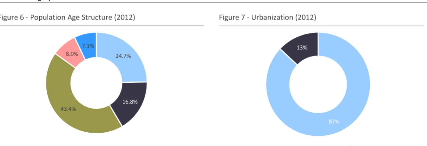
Figure 6 - Population Age Structure (2012) Figure 7 - Urbanization (2012)

Source: IBGE, World Bank

Figure 3 – GDP Real Growth Rates Comparison

24.7%

16.8%

43.4% 8.0%

7.1%

0-14 years 15-24 years 25-54 years 55-64 years + 65 years

10.9% 9.6% 8.3% 8.4% 7.4% 6.8% 6.8% 5.3%_{4.7% 4.6% 4.3%} 240 260 300 350 380 415 465 510 545 612 678 2003 2004 2005 2006 2007 2008 2009 2010 2011 2012 2013

Unemployment Rate (%) Nominal Minimum Wage (R$) 0.9% 2.3% 1.4% 1.3% -4.0% -2.0% 0.0% 2.0% 4.0% 6.0% 8.0% 10.0%

Brazil GDP (%) Advanced Economies GDP (%)

2.1 2.2 2.5 2.7 3.6 4.9 9.2 16.8 Russia Brazil United Kingdom France Germany Japan China United States 87% 13%

(24)

3.2 THE BRAZILIAN FOOTWEAR INDUSTRY

3.2.1 Brief History

Brazil, the largest country in Latin America, holds the 3rd_{position in the ranking of world}

footwear manufacturers, with production mostly destined to supply the domestic market, the 4th_{largest in the world.}

The economic development of the Brazilian footwear industry began in Rio Grande do Sul (RS), one of the southern states of the country, with the arrival of the first German immigrants in 1824. Having settled in Vale dos Sinos, RS, they brought with them the crafts culture particularly of leather goods. The first Brazilian footwear factory appeared in 1888 and year-by-year, the state of Rio Grande do Sul developed to become one of the largest footwear clusters worldwide.

Although the concentration of large size companies is located in the state of Rio Grande do Sul, the Brazilian footwear industry is gradually being developed in other regional poles. Particularly to the Southeast, in the inland of São Paulo state (cities of Jaú, Franca and Birigui), and the Northeast (states of Ceará and Bahia), where there are fiscal incentives and a vast and cheaper workforce. Footwear production is also growing in the states of Santa Catarina and Minas Gerais. 34,0% 35,0% 29,6% 1,3% 0,1% 40,9% 7,7% 48,4% 2,8% 0,2%

(1) IBOPE estimates for consumption growth rates between 2011 and 2012

SOUTHEAST 55.3% of Country’s GDP 6.5% Consumption Growth1 SOUTH 16.5% of Country’s GDP 19.7% Consumption Growth1 MIDWEST 9.6% of Country’s GDP 19.4% Consumption Growth1 NORTH 5.1% of Country’s GDP 26.5% Consumption Growth1 NORTHEAST 13.5 % of Country’s GDP 24.1% Consumption Growth1

Figure 10 - Footwear Companies by Region

Source: Brazilian Footwear Association (“Abicalçados”)

Source: IBGE, Brazilian Institute of Public Opinion and Statistics (“IBOPE”)

(25)

The industry is composed by over 8,000 manufacturers, which produce more than 800 million pairs of shoes per year, being c. 120 million destined to exports to more than 140 countries, and the remaining 680 million to supply the domestic demand. The United States and Argentina are the major consumers of Brazilian shoes, accounting together for c. 28% of total exports value. The Brazilian footwear industry is recognized by the quality and high specialization within different and complex categories, representing an important player in the women’s shoe segment worldwide. The industry has been evolving, in the recent years, in order to increase the value of its products and to create competitive advantages over the expanding Asian players in the country.

3.2.2 Footwear Retail Market

The Brazilian footwear market reached R$40.2 billion in 2012 at the retail level and is expected to grow at a CAGR15_{of 6.8% over the next four years, reaching an estimated R$50.8 billion in}

2017. Although sizeable, this segment has still much room to grow and it seems like a matter of time for the still low footwear consumption per capita, in the country, of 3.8 pairs per year to close some of the existing gap between the developed economies such as the US (with 7.2 pairs per capita) or France (with 6.7 per year).

As it was previously stated, approximately 85% of the Brazilian overall shoe production is destined to the domestic market, a clear evidence of the strong consumption potential of the country. Recent macroeconomic conditions like favorable demographics and increasing consumers’ income have been boosting this consumption capacity. Brazil has a young population of more than 65% of Brazilians, or 130 million people under 39 years old, who are

15_{Compounded annual growth rate}

31,0 33,5

37,7 38,9 40,2

42,2 45,1

48,4 51,4 54,8

2008 2009 2010 2011 2012 2013E 2014E 2015E 2016E 2017E

Figure 12 – Footwear Consumption per Capita (2012)

1.8 2.0 2.2 3.8 5.3 5.4 5.7 5.9 6.7 7.2 India China Indonesia Brazil Germany Japan Italy United Kingdom France USA CAGR13-17: 6.8% 18.6% CAGR08-12: 6.7% 18.6%

Figure 11 – Footwear Retail Sales

(26)

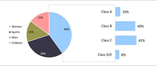
40% 30% 15% 15% Women Sports Men Children

the focus of the apparel and footwear sales. Additionally, in the past few years, the country has been witnessing an increasing participation of women in the workforce, a segment responsible for approximately 40% of total footwear consumption. This economic empowerment and financial independence among Brazilian women has been a key driver for women’s footwear and apparel industry growth.

The industry is characterized by high income-elasticity, meaning that with increasing purchasing power individuals tend to increase their expenses with clothes and footwear products. The Brazilian economic momentum of the past recent years has led to the emergence of a preponderant middle-class, which created a massive consumption potential especially among the population of social classes B and C.

Lower-income consumers make up the largest share of the Brazilian population. Rising incomes and living standards offer plenty of potential to retailers. The fastest growing social class is class D, essentially, the lower middle class. Upwardly mobile consumers, now enjoying improved lifestyles coupled with an increased purchasing power, although incomes remain

Figure 13 – Footwear Consumption by Segment (2012)

8% 42% 40% 10% Class D/E Class C Class B Class A

Figure 14 – Industries Income Elasticity Source: APLAC, Mintel Study (2013)

(27)

relatively low, drive most of class D expansion. Between 2008 and 2018, the number of Brazilians consumers living on annual gross income less than US$ 5,000 is expected to drop by one fifth. As lower-end incomes improve, apparel and footwear retailers in Brazil are changing their offer to tap into the potential of this emerging consumer group.

The footwear retail market in Brazil is highly fragmented, consisting of approximately 29,000 footwear retail companies. Such fragmentation is well funded in a sector marked by few specialized and capitalized chain players, regional competition and neighborhood reach.

There is a wide variety of footwear store categories such as specialized stores and family-run businesses, department stores, and even supermarkets sell shoes. Although the family-run businesses are still the largest type of stores within the Brazilian market, these unstructured retailers are losing space as some emerging large players start to capitalize and expand their operation. Online stores, for example, have become an important sales channel for footwear products, especially among the young consumers due to the considerable increased

exposure to technology and internet in past recent years.

It is interesting to note that the women footwear market in Brazil is characterized by the limited presence of imported products and brands, except when one considers the niche of high-income consumers. Despite Brazil’s booming middle class and demand for international brands, very few foreign companies are well established in the country due to the successful fast-fashion model adopted by most of the leading national players that makes it very hard for the international products to be competitive. The market’s high operation costs, the inefficiencies arising from the distance between the production site abroad to the retail stores, and the high import tariffs are key barriers for an international player to enter in the country. Moreover, the cultural particularities of a large and diversified country like Brazil are quite hard to identify and adapt when is a foreigner player trying to develop products for the Brazilian population.

Less reliant on imports, domestic chains can position themselves at the lower-end of the price spectrum, making it easier for them to move into markets where incomes may be raising, but have not yet reached the same level as in larger cities.

Figure 15 – Footwear Distribution Channels

77,3%

14,5%

4,3% 3,9%

Specialist Retailers Department Stores

Hypermarkets, Supermarkets & Discounters Other

(28)

Additionally, most leading footwear retailers in Brazil operate under a hybrid model of proprietary and franchised stores with the latter accounting for most of the stores base. Part of the reason for Brazil’s comparatively high number of apparel and footwear specialists is the urbanized landscape of the country. In 2011, 85% of Brazilians lived in urban areas, a higher percentage than in many markets such as the US and other BRIC nations. However, the 10 largest cities account for only one fifth of the urban population. This means that, although there are a high number of locations able to support apparel and footwear specialist stores, gaining a regional or national coverage requires a larger network, which explains the need for the franchise model.

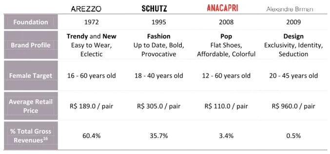
To conclude,Figure 16 presents a fashion/price positioning of the main footwear players in the country, as well as the positioning of Arezzo&Co brands: Arezzo, Schutz, Anacapri and Alexandre Birman. Please refer to the appendix for a brief description of some of these companies.

Figure 16 – Positioning of Main Footwear Players in Brazil

(29)

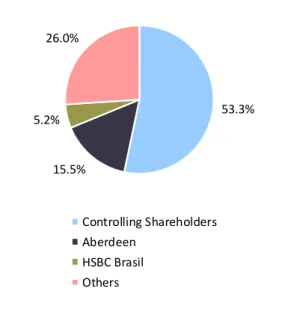
53.3% 15.5% 5.2% 26.0% Controlling Shareholders Aberdeen HSBC Brasil Others 3.3 COMPANY OVERVIEW 3.3.1 Company’s History

Established in 1972, in the city of Belo Horizonte, Minas Gerais, by the brothers Anderson and Jefferson Birman, Arezzo&Co grew up to become a market leader in the women footwear and accessories industry in Latin America. The first milestone to consolidate its first brand Arezzo in Brazil’s women footwear industry was in 1979 with the launch of the Anabela sandal, covered in jute thread that soon became a best-seller in the country.

In the 80’s the company switched its production to a vertically integrated model, enabling a greater quality control throughout the entire manufacturing process, from the production of leather and soles to the finished product. In 1990, Arezzo&Co started to enhance its investments in the creation of own retail stores as well as in the development of a franchise business model, extending its sales network to the countryside areas of Brazil. Still in the 90’s the company closed its operation in Minas Gerais and replaced it with a hybrid production model, combining both internal and outsourced production, in Vale dos Sinos, Rio Grande do Sul. The company also transferred its commercial operations to São Paulo and adopted the fast-fashion concept, developing 7 to 9 different collections every year.

In the 2000’s, Anderson Birman acquired his brother’s share of the company and incorporated his son’s own brand, Schutz, creating together with the already existing brand Arezzo, the Arezzo&Co group. Also by this time, the company expanded its brand portfolio creating Anacapri and Alexandre Birman brands aiming at targeting new consumer segments.

In 2007, the Brazilian private equity Tarpon acquired a minority stake in the company, helping with the development of its corporate structure and governance standards. Four years later, in 2011, Arezzo&Co became a public company with its shares traded at Novo Mercado, the highest level of corporate governance of São Paulo Stock Exchange (BM&F Bovespa). In 2012, Tarpon sold its entire stake in Arezzo&Co, being no longer part of the company. As of December 2013, the controlling shareholders, Anderson Birman and his son, Alexandre Birman, held together approximately 53.3% of the Company’s shares, with the remaining 46.7% being free float.

Figure 17 – Ownership Structure (2013)

(30)

3.3.2 Brands’ Positioning

Arezzo&Co is a multi-brand company, with different brands targeting particular consumer groups and usage occasions. The strong platform of brands, Arezzo, Schutz, Anacapri and Alexandre Birman, enables the company to capture growth from different income segments with no cannibalization between them. Over the past five years, Arezzo&Co has been able to increase its market share in Brazil’s women footwear industry, representing c. 11%, in 2012, according to Euromonitor research.

Arezzo and Schutz are the most significant brands, accounting together for more than 96% of Arezzo&Co total gross revenues. This two brands aim at targeting consumers from income-classes A and B, which are currently benefiting from their large disposable income for discretionary products, like footwear and apparel. Anacapri brand was launched in 2008 and it targets a lower and broader income consumer group offering more casual, lower priced shoes and accessories. On the opposite side of the spectrum, Alexandre Birman, created one year later, targets higher price points as well as more fashionable and formal occasions.

16_{2013 Total Gross Revenues, including international and domestic operations}

Foundation 1972 1995 2008 2009

Brand Profile

Trendy and New

Easy to Wear, Eclectic Fashion Up to Date, Bold, Provocative Pop Flat Shoes, Affordable, Colorful Design Exclusivity, Identity, Seduction

Female Target 16 - 60 years old 18 - 40 years old 12 - 60 years old 20 - 45 years old

Average Retail

Price R$ 189.0 / pair R$ 305.0 / pair R$ 110.0 / pair R$ 960.0 / pair

% Total Gross

Revenues16 60.4% 35.7% 3.4% 0.5%

Figure 18 – Arezzo&Co Market Share

Figure 19 – Company Brands and Positioning (2013)

4% 7% 8% 9% 10% 11% 2007 2008 2009 2010 2011 2012 Source: Arezzo&Co Source: Arezzo&Co

(31)

5,063

6,455 7,533

8,980 10,008

2009 2010 2011 2012 2013

Number of Pairs Sold ('000)

8.9%

91.1%

Owned Factory Others

Shoe Pairs ('000) 10,008 Handbags ('000) 642 3.3.3 Business Model

The company operates a very flexible business model, in which all shoes and accessories are designed internally but its production can be either handled internally or outsourced to leading footwear industries in the country. Currently, approximately 91.1% of the production is outsourced to third parties while the remaining 8.9% is manufactured in-house. In 2010, these figures were 84.2% and 15.8%, respectively for outsourced and in-house production, which highlights the company’s confidence towards a more outsourced production structure.

However, Arezzo&Co does not simply outsource its production to third parties. It has full control over each shoe’s design, brand, prototype development and even raw material selection. The company’s scale and asset light structure gives it flexibility to source a large number of SKUs17_{from various factories on a short period and at competitive prices. Every year, the}

company develops approximately 11,500 models that are gradually filtered by product development and sales teams to finally manufacture and deliver to stores roughly 6,000 models within 7 to 9 different collections per year.

With an annual average growth rate of 18.6% between 2009 and 2013, Arezzo&Co hit the record mark of 10 million sold pairs of shoes, with 10,008 thousand pairs and 642 thousand handbags sold in 2013.

17_{SKU – Stock Keeping Unit}

Figure 20 – Sourcing Model

Figure 21 – Evolution of the Number of Pairs Sold Figure 22 – Number of Shoes and Handbags Sold (2013) CAGR09-13: 18.6%

Source: Arezzo&Co

(32)

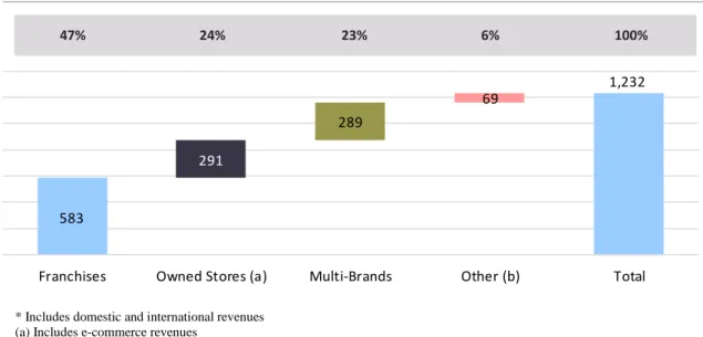
Arezzo&Co’s flexibility is also found at the distribution level, in which the company operates a multiple distribution model combining owned, franchised and multi-brand stores, as well as an e-commerce platform. Arezzo&Co brands are also found in over 50 countries worldwide through multi-brand and department stores. Arezzo&Co distribution model allows the company to determine the most profitable combination among channels, widens stores capillarity and brands’ visibility.

* Includes domestic and international revenues (a) Includes e-commerce revenues

(b) International revenues and other revenues in the domestic market

Arezzo&Co own stores are strategically located to leverage sales and stand as a way to improve the company’s knowledge on retail best practices and point-of-sale (“PoS”) management through the direct contact with costumers. The company domestic owned stores are mainly located in São Paulo and Rio de Janeiro and, on average, present an annual revenue per store 1.5x higher than a franchised store.

On the other hand, the franchise model allows for a rapid expansion with relatively low capital disbursement. Franchise stores are adapted to the specific necessities of each region and are geared towards attaining high profitability levels, enabling the company’s footprint presence at geographic areas where it would not make economic sense for own stores. Arezzo&Co franchise model has been consistently awarded the Franchising Excellence Stamp from the Brazilian Franchising Association (ABF) since 2004.

Finally, the multi-brand retail stores and e-commerce platform consolidate the strength of the other distribution channels by increasing the capillarity in small-size cities. Sales through these channels reach all the Brazilian states, as well as around 50 countries abroad, including Portugal.

583

1,232

291

289

69

Franchises Owned Stores (a) Multi-Brands Other (b) Total

Figure 23 – Gross Revenues* Breakdown by Channel (2013) – R$ million

47% 24% 23% 6% 100%

(33)

3.3.4 Evolution of the Key Operating and Financial Indicators

Over the last 4 years, Arezzo&Co gross revenues have been growing four times faster than the footwear retail market in Brazil, with a CAGR09-13 of 24.5%. This is the result of the company’s

primary growth strategy of enhancing its position as a fast fashion retailer, bringing the newest trends quickly to the market, at affordable prices, through an expanding network of owned and franchised retail stores, in the domestic market. Currently, the company has c. 2,077 employees and its international operations account for only 5% of total gross revenues.

In 2013, the Company reached a total number of 449 domestic stores, of which 54 owned stores and 395 franchised stores (totaling approximately 32,000sqm of sales area) and 9 international stores. This represents an annual average growth rate of 14.3% of the total number of stores of the company, between 2009 and 2013.

Arezzo&Co successful retail oriented structure, through its three distribution channels, has allowed the company to quickly expand its presence throughout the country. Currently the most relevant distribution channel is the franchise model, accounting for 49.8% of domestic gross revenues. After the IPO, the company concentrated in the development of its own network of retail stores in order to have a better control over its brands awareness and costumers interaction. Currently, the own stores distribution channel represents c. 24.9% of total revenues, from the 15.0% it represented back in 2009.

Arezzo&Co sales through the multi-brand stores channel represented 24.7% in 2013, which corresponds to 2,451 multi-brand stores across the country. This channel enhances brands capillarity and fills the gap left by franchised and own stores, which consequently helps in the consolidation of the brands.

513

713

863

1,109 1,232

2009 2010 2011 2012 2013

Total Gross Revenues (R$ '000)

242 267 289 334 395 21 29 45 56 54 14,920 17,558 21,821 26,543 31,848 2009 2010 2011 2012 2013

Owned Stores Franchise Stores

Sales Area - Total (sqm) Figure 24 – Total Gross Revenues Evolution Figure 25 – Number of Stores Evolution

CAGR09-13: 24.5%

(34)

Arezzo&Co operates a strong portfolio of brands that allow it to capture growth from different income segments and growth strategies. Arezzo is the most developed and consolidated brand, with an already strong penetration among the multiple distribution channels of the company. In 2013, the flagship brand represented approximately 61.2% of the company’s total domestic gross revenues and had a total sum of 357 franchised and owned stores in every state of the country.

Schutz is the company’s second most premium brand that has started with a go-to market strategy relying upon independent multi-brand stores. Although being an efficient strategy from a returns perspective, it hampers brand’s development when you have no control of the point-of-sale. Thus, since the IPO, Arezzo&Co has been investing in the development of Schutz mono-brand stores – first through flagship and owned stores and then, in 2012, with the roll out of the franchise model for the brand. Currently, Schutz brand represents 34.4% of total domestic revenues and is present in more than 65 owned and franchised stores.

The remaining 4.4% domestic revenues come from Anacapri and Alexandre Birman brands. Anacapri brand holds eight own stores in São Paulo and is sold in multi-brand stores throughout the country. Similar to what it did with Schutz, the company has recently started to develop the franchise model of Anacapri with 15 franchised stores opened by the end of 2013. Alexandre Birman has only two owned stores located in São Paulo and its products can be found at leading luxury retail stores in Brazil and abroad, such as in Saks Fifth Avenue and Bergdorf Goodman, in New York.

The above-explained strategy allowed the company to increase its net revenues (gross revenues minus the taxes on revenues) at an average annual growth rate of 23.6% between 2009 and 2013. 55.7% 54.1% 51.5% _47.9% 49.8% 28.5% 28.4% _28.7% 26.7% 24.7% 15.0% 16.6% 18.7% _23.9% _24.9% 0.8% 0.8% 1.1% 1.4% 0.6% 2009 2010 2011 2012 2013

Franchise Multi-Brand Owned Stores Others

Figure 26 – Domestic Gross Revenues by Channel Evolution Figure 27 – Domestic Gross Revenues by Brand (2013)

61%

34%

4%

Arezzo Schutz Other Brands