How does banking industry influence economic growth in Latin American countries?

(1)

M

ASTER OF

S

CIENCE IN

F

INANCE

M

ASTER

’

S

F

INAL

W

ORK

D

ISSERTATION

H

OW DOES BANKING INDUSTRY INFLUENCE ECONOMIC

GROWTH IN

L

ATIN

A

MERICA

?

K

ONSTANTIN

P

ETROVICH

T

RETYAKOV

S

UPERVISOR

(

S

):

Maria Cândida Rodrigues Ferreira

(2)

1. Introduction

Financial sector of many Latin American countries experienced significant reforms in the early 1990s. During that time a lot of national banks were privatized, capital markets were developed by the means of creating domestic securities and exchange commissions, improving regulatory and supervisory frameworks, and enhancing market operations, such as securities clearance, custody arrangements, accounting and information disclosure. Government control over banks was highly reduced. Barriers to the entry of foreign banks were eliminated. Financial liberalization index developed by Kaminsky and Schmuckler (2003) and updated by Galindo et al. (2006) demonstrates a huge increase in value for Latin American countries starting from year 1988. Hermes and Nhung (2010) find strong support for the positive impact of financial liberalization programs on bank efficiency in Latin America.

The elimination of the government control and intervention aims at restoring and strengthening the price mechanism, as well as conditions for market competition (Hermes and Lensik 2005). Competitive pressure stimulates banks to become more efficient by reducing overhead costs, enhancing the level of bank management, improving risk management, and offering new financial instruments and services (Denizer et al. 2000). Moreover, if domestic financial markets are opened up to foreign competition, this will further increase pressures to reduce costs, whereas at the same time, new banking and risk management techniques, and new financial instruments and services may be imported (Claessens et al. 2001).

Financial sector that is more efficient and productive fulfils its functions better. The primary function of the financial sector is to “facilitate the allocation of resources

(4)

2

across space and time in a certain environment” (Levine 1997, p.691). Financial development also decreases market frictions that result from imperfect information by connecting savers with investors and by allocating resources to profitable projects (Demirgüç-Kunt 2006). Therefore, the financial sector plays a crucial role in the economy because it provides relevant information, monitors investment projects, promotes risk diversification, increases the amount of transactions, and affects any entrepreneurial and trading activity (Levine 2005).

There are many studies on the relationship between financial development and economic growth. For example Levine (2005) concludes that financial development causes economic growth. And the channels through which financial development causes economic growth are productivity and capital accumulation (Beck et al. 2000). Furthermore the mechanisms through which savings are channelled to productive investments do exist. These mechanisms involve both financial intermediaries (mostly banking institutions, for indirect financing) and financial markets (for the direct financing) (Maudos and Fernandez de Guevara 2006).

In this paper we are testing the importance of banking sector efficiency and profitability as well as its market concentration to economic growth of Latin American countries via an approach similar to the one of Ferreira (2012). In order to test this relationship we will consider model specifications developed by Rajan and Zingales (1998) and later contributions by Claessens and Laeven (2004, 2005).

However, in contrast to these authors we will not consider the influence of the external financial dependence, but instead we will estimate the effects on

(5)

3

economic growth of bank efficiency, bank market concentration and bank profitability.

The test is going to embrace various components of GDP (Gross Domestic Product): final consumption expenditure, gross fixed capital formation, exports of goods and services and imports of goods and services.

The data sample is represented by a panel of 10 Latin American countries with observations ranging from year 1998 till year 2012. This time period follows the era of financial liberalization in many Latin American countries, and thus is likely to capture the evolution of the financial sector after the reforms.

According to our knowledge, our study is unique because this is the first time a researcher seeks to explain economic growth in the Latin American region with the variables that we consider: bank efficiency, bank market concentration and bank profitability.

Our findings point at insignificant influence of the bank cost efficiency and bank market concentration on economic growth of Latin American countries. This result is obtained for GDP and all of its components in the analysis. The reason for this may be the fact that the economies in Latin America are less dependent on the banking sector (when measured by the percentage of domestic credit provided by the financial sector to GDP). However bank profitability measured by return on assets and return on equity appears to be an important factor for explaining economic growth. The evidence of statistically significant positive effects has been found for GDP itself and for all of its components.

(6)

4

2. Brief literature review

With the release of King and Levine’s paper in 1993 a large number of studies explaining countries’ output variables with financial ratios such as liquid liabilities, bank loans to private sector as percentage of GDP, monetary aggregates and stock market capitalization were born. Cross-country empirical analyses support the supply-leading hypothesis by showing that the exogenous component of financial development has a positive effect on economic growth (Beck et al. 2000; Benhabib and Spiegel 2000; Khan and Senhadji 2003), productivity, and capital accumulation (King and Levine 1993; Beck et al. 2000; Nourzad 2002; Rioja and Valev 2004a). Analyses at the firm-industry level also support the argument that financial development is conducive to growth (Rajan and Zingales 1998; Beck 2002; Love 2003; Manning 2003; Kroszner et al. 2007). Moreover, Beck et al. (2004) conclude that financial development is not only growth but also pro-poor, that is, in countries with better-developed financial intermediation, income inequality declines faster.

Some authors provide evidence that financial development has no significant effect on economic growth (Shan 2005). Others argue that the effect is dependent on certain conditions (Rioja and Valev 2004a,b) and that financial development may have a negative effect in some cases, depending on the time frame considered (Loayza and Ranciere, 2006).

Although there is an extensive amount of studies showing that financial development causes economic growth, others assert that financial development is just the consequence of economic growth. As stated by Shan et al. (2001), the relationship between financial development and economic growth may be a ‘‘chicken and the egg’’ problem, since financial institutions are usually developed

(7)

5

in developed countries (DCs) and underdeveloped in less developed countries (LDCs). The theoretical explanation behind this hypothesis is that there is a virtuous cycle in developed economies, where an expansion in the real sector increases the demand for loanable funds (Greenwood and Jovanovic 1990; Berthélemy and Varoudakis1996).

Some empirical analyses show bidirectional causality between financial development and economic growth (Berthélemy and Varoudakis 1996; Demetriades and Hussein 1996; Luintel and Khan 1999; Calderón and Liu 2003). There is also empirical evidence that the effect of financial development on economic growth is different across regions (Al-Awad and Harb 2005; Iyare et al. 2005; Habibullah and Eng 2006; Naceur and Ghazouani 2007; Odhiambo 2007), income levels (Jung 1986; Ram 1999; Xu 2000; Andersen and Tarp 2003; Rioja and Valev 2004a; Aghion et al. 2005), levels of financial development (Rioja and Valev 2004b), and institutions (De Gregorio and Guidotti 1995; Shen and Lee 2006).

Several studies for the relationship between financial development and economic growth have been done for Latin American countries. De Gregorio and Guidotti (1995) in a panel data set for 12 Latin American countries between 1950 and 1985 find a significant negative correlation between financial intermediation and growth. They argue that this is due to incorrect policies in the field of regulation of the financial sector.

Blanco (2009) performs a Granger causality test taking a sample of 18 Latin American countries from 1962 to 2005. She finds a unilateral relationship between financial development and economic growth. The natural logarithm of private credit issued by banks as a share of GDP is the measure of financial development

(8)

6

used in this paper. However, if the sample is divided according to different income levels and institutional quality, then there is two-way causality between financial development and economic growth only for the middle income group and for countries with stronger rule of law and creditor rights. A later study (Blanco 2013) for a panel of 16 Latin American countries during the 1961-2010 period shows a statistically significant positive effect of financial development on economic growth in the long-run for high-income countries but a negative significant effect for low-income countries. In this paper financial development is measured by private credit to GDP ratio as well.

Hermes and Nhung (2010) investigate the relationship between financial liberalization and bank efficiency using a data sample for 10 emerging economies in the period from 1991 till 2000. Among the countries under consideration are Argentina, Brazil, Mexico and Peru. The authors find strong support for the positive impact of financial liberalization programs on bank efficiency.

Chortareas et al. (2010) provide evidence of consolidation of the financial systems in Latin America as a response to changes in the regulation. More concentrated banking sector was a result of this process of consolidation. They analyze a panel data sample for 9 Latin American countries in the period between 1997 and 2005 in order to explore the effect of market structure and bank efficiency on the banking performance, which is measured by Return on Assets ratio. The conclusion is that banks’ profits do not seem to be explained by market power. But in contrast, efficiency seems to be the main driving force of increased profitability for most Latin American countries.

Studies revealing the importance of bank market concentration to economic growth were performed by Cetorelli and Gambera (2001) and Ferreira (2012),

(9)

7

among others. They reveal negative influence of bank market concentration not only on GDP, but also on its components.

If we look at the studies on the effects of bank market concentration in Latin America we shall point out that Yeyati and Micco (2003) come up with a conclusion that changes in the market structure after the reforms of 1990’s did not give rise to a less competitive industry.

Chortareas et al. (2012) show that bank market concentration in Latin American countries has little or no influence on interest margins, which are often considered as a proxy for bank efficiency.

3. Methodology and data

3.1 Basic model

To test the influence of bank efficiency and market concentration on economic growth we employ generalized least squares regression (GLS) approach with random effects.

We consider model specifications introduced by Rajan and Zingales (1998) and later contributions by Claessens and Laeven (2004, 2005) to construct our model for the estimation. Similar to Ferreira (2012) we will test the influence of bank efficiency, bank market concentration and bank profitability on GDP growth and on its components: final consumption, investment, exports and imports.

The equation to estimate is the following:

(10)

8 Where:

Growth = natural logarithm of the GDP, or of one of its components: final consumption, gross fixed capital formation, exports or imports of goods and services;

i = Latin American country (i = 1, ... 10); t = year (t = 1998, ..., 2012);

lag1 growth = first lag (t-1) of the growth endogenous variable;

bank efficiency = natural logarithm of the Data Envelopment Analysis (DEA) technical efficiency score;

bank market concentration = natural logarithm of the Herfindahl-Hirschman Index (HHI);

bank profitability = return on assets (ROA) or return on equity (ROE). All financial and bank performance variables are sourced from the Bankscope database (annual data from consolidated accounts of commercial, investment and savings banks; all in nominal values and in United States dollars).

The macroeconomic data is sourced from World Bank, and includes: Gross Domestic Product (GDP), final consumption expenditure, gross fixed capital formation, exports of goods and services and imports of goods and services1. The sample of Latin American countries is represented by a panel of data with yearly observations for banks of Argentina, Bolivia, Brazil, Colombia, Costa Rica, Dominican Republic, El Salvador, Haiti, Peru and Venezuela for the time period

1

GDP at purchaser's prices is the sum of gross value added by all resident producers in the economy plus any product taxes and minus any subsidies not included in the value of the products. It is calculated without making deductions for depreciation of fabricated assets or for depletion and degradation of natural resources. Data are in current U.S. dollars. Dollar figures for GDP are converted from domestic currencies using single year official exchange rates. For a few countries where the official exchange rate does not reflect the rate effectively applied to actual foreign exchange transactions, an alternative conversion factor is used. The data for GDP components is given as percentage of GDP.

(11)

9

from 1998 till 2012. The choice of these particular countries is explained by the data availability in the Bankscope database considering our model specifications2. Table I brings together the distribution of GDP weights of Latin American countries for the period from year 1998 till year 2012. The 10 selected countries are listed in bold type and represent about 60% of Latin America economy according to the historical average.

Relative dynamics of countries’ GDPs can be observed in Table I. Obviously for countries with large economies, such as Argentina, Brazil and Mexico, the changes in their GDP shares will be more sensible to the year-on-year changes in GDP numbers. For example the consequences of Argentinian default in December 2001 may be noticed by the slump from 12.4% of Latin American economy in 2001 to 5.25% in 2002. Since then Argentina amplifies its share in Latin American economy up to 8.28% in 2012. Brazil experienced a sharp decline in its GDP share from 38.06% in 1998 to 29.26% which is related to its currency devaluation. Since 2002, when Luis Inácio Lula da Silva won the presidential elections, Brazil’s economy is growing fast from 25.94% in 2002 up to 43.14% in 2011 with moderate decline in 2012 down to 39.23%. Mexican GDP share grows rapidly from 22.91% in 1998 to 38.61% in 2002, since then Mexico loses its position down to 20.52% in 2012. It can be explained by the considerable expansion of the Brazilian economy.

2

Including at least Mexico in the sample would have made a great contribution into the study since this country represents a large share of Latin American economy, but unfortunately the values for personnel expenses in Mexico are not reported in the Bankscope database.

(12)

10

Table I. Gross Domestic Products of Latin American countries. (in percentages to their sums).

1998 1999 2000 2001 2002 2003 2004 2005 2006 2007 2008 2009 2010 2011 2012 Argentina 13.49 14.14 12.80 12.40 5.25 6.49 6.69 6.62 6.61 6.85 7.39 7.38 7.19 7.77 8.28 Bolivia 0.38 0.41 0.38 0.38 0.41 0.40 0.38 0.35 0.35 0.34 0.38 0.42 0.38 0.42 0.47 Brazil 38.06 29.26 29.03 25.54 25.94 27.67 29.00 31.87 33.64 35.92 37.44 38.95 41.77 43.14 39.23 Chile 3.58 3.64 3.57 3.34 3.65 3.90 4.40 4.49 4.78 4.55 4.07 4.13 4.24 4.38 4.70 Colombia 4.44 4.30 4.50 4.53 5.04 4.74 5.11 5.29 5.03 5.45 5.53 5.63 5.59 5.86 6.44 Costa Rica 0.64 0.79 0.72 0.76 0.87 0.88 0.81 0.72 0.70 0.69 0.68 0.71 0.71 0.71 0.79 Cuba 1.16 1.41 1.38 1.46 1.73 1.80 1.67 1.54 1.63 1.54 1.38 1.49 1.25 1.19 1.26 Dominican republic 0.96 1.08 1.08 1.15 1.37 1.07 0.97 1.23 1.11 1.09 1.04 1.12 1.01 0.97 1.03 Ecuador 1.18 0.95 0.83 1.13 1.47 1.62 1.60 1.50 1.45 1.34 1.40 1.50 1.32 1.34 1.46 El Salvador 0.54 0.62 0.59 0.64 0.74 0.75 0.69 0.62 0.57 0.53 0.49 0.50 0.42 0.40 0.42 Guatemala 0.87 0.91 0.87 0.86 1.07 1.10 1.05 0.98 0.93 0.90 0.89 0.91 0.81 0.83 0.87 Haiti 0.17 0.20 0.17 0.16 0.17 0.14 0.16 0.15 0.15 0.16 0.15 0.16 0.13 0.13 0.14 Honduras 0.23 0.27 0.32 0.35 0.40 0.41 0.38 0.35 0.33 0.32 0.31 0.35 0.31 0.31 0.32 Mexico 22.91 29.25 31.17 33.84 38.61 36.17 33.85 31.44 29.85 27.42 24.89 21.52 20.41 20.20 20.52 Nicaragua 0.21 0.24 0.23 0.25 0.27 0.27 0.25 0.23 0.21 0.20 0.19 0.20 0.17 0.17 0.18 Panama 0.49 0.57 0.52 0.54 0.63 0.65 0.62 0.56 0.53 0.52 0.52 0.58 0.52 0.55 0.63 Paraguay 0.41 0.42 0.37 0.35 0.33 0.33 0.35 0.32 0.33 0.36 0.42 0.38 0.39 0.45 0.44 Peru 2.56 2.57 2.40 2.49 2.92 3.07 3.05 2.87 2.86 2.82 2.93 3.13 3.07 3.15 3.55 Puerto Rico 2.44 2.88 2.78 3.19 3.68 3.75 3.46 2.99 2.66 2.32 2.10 2.29 1.89 1.72 1.77 Uruguay 1.15 1.20 1.03 0.96 0.70 0.60 0.60 0.63 0.60 0.62 0.69 0.73 0.76 0.81 0.87 Venezuela 4.12 4.88 5.28 5.67 4.78 4.19 4.91 5.26 5.67 6.05 7.15 7.92 7.68 5.51 6.64 SUM ALL 100 100 100 100 100 100 100 100 100 100 100 100 100 100 100 SAMPLE % 65.36 58.25 56.94 53.71 47.47 49.41 51.78 54.97 56.69 59.91 63.16 65.91 67.94 68.07 66.97 AVERAGE SAMPLE % 59.10

(13)

11

3.2 Bank efficiency

Techniques based on estimation of efficiency frontiers allow for solving such an optimization problem as finding the best bank to operate in the market. The frontiers are calculated from the given inputs and outputs of the production process. Each unit’s efficiency is measured by the distance from the frontier. Two types of methods are applied in most of empirical studies for measuring bank efficiency: parametric and non-parametric. Stochastic Frontier Analysis (SFA) is usually used for studies based on parametric method. Data Envelopment Analysis (DEA) is mostly adopted as non-parametric method of drawing an efficiency frontier. The DEA frontier is formed by the “best-practice observations” yielding a convex production possibility set. Since our focus lies on the cost side of banking operations, we employ an input-oriented, constant-returns-to-scale (CRS) model and the variable that is computed is technical efficiency (TE). Technical efficiency can be defined as deviation from the efficient cost frontier due to inefficient input utilization. In order to obtain the DEA input-orientated CRS efficiency scores the following optimisation problem is solved:

(2)

subject to:

(3) (4) (5)

(14)

12

Here θ is a scalar and λ is a vector of constants. yi is the output vector for the

DMUi (Decision Making Unit) and Y is the matrix of outputs of the other DMUs. xi is

the vector of inputs of the DMUi and X is the matrix of inputs of the other DMUs. In

our case DMUs are represented by consolidated bank accounts on the national level. The number of DMUs ranges from i=1…n according to the number of countries in the sample. For more specifications on the DEA model see Coelli et.

al. (2005) and Thanassoulis et al. (2008).

In this paper the following inputs are considered:

1. Price of borrowed funds = natural logarithm of the ratio Interest Expenses on Customer Deposits over Total Deposits.

2. Price of physical capital = natural logarithm of the ratio Non-Interest Expenses over Fixed Assets

3. Price of labor = natural logarithm of the ratio Personnel Expenses over Total Assets3.

The outputs are:

1. Loans = natural logarithm of Total Loans.

2. Securities = natural logarithm of Total Securities.

3. Other earning assets = natural logarithm of the difference between Total Earning assets and Total Loans.

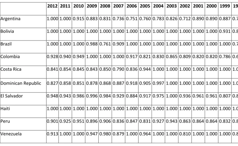
Efficiency scores for the sample of ten Latin American countries are presented in Table II. Throughout the time period considered bank efficiency mainly increased across the countries. The only countries where efficiency decreased are Costa Rica and Dominican Republic. Haitian and Bolivian banks appear to be the most

3

Due to the absence of the Number of Employees variable for some countries, the ratio Personnel Expenses over Total Assets is used as a proxy for labour prices. This approach is also followed by Weill (2004) among others.

(15)

13

efficient across time in this dataset. However we should keep in mind that these countries are relatively small in terms of their economies, and therefore economies of scale should be taken into consideration when one is comparing these results to the other countries’ efficiency scores.

It is remarkable that in Table II Brazil stays on the efficient frontier 11 times out of 15 despite the fact that its net interest rate margins4 are the highest in Latin American region (Chortareas et al. 2012). So, we argue that Brazilian banks’ high interest rate margins are not a very inefficient issue.

In the most recent years (2010-2012) Argentina and Brazil appear on the efficient frontier. It can be interpreted as an indicator of improving financial markets in Latin America generally, since its leading economies succeeded in establishing efficient banking sectors.

4

Net Interest Rate Margin (NIM) =

. NIM is a measure of interest rate

spreads of commercial banks, and is widely used as a proxy for bank efficiency (e.g. Herrero et al. 2002).

(16)

14

Table II. Data Envelopment Analysis cost efficiency measures.

2012 2011 2010 2009 2008 2007 2006 2005 2004 2003 2002 2001 2000 1999 1998 Argentina 1.000 1.000 0.915 0.883 0.831 0.736 0.751 0.760 0.783 0.826 0.712 0.890 0.890 0.887 0.745 Bolivia 1.000 1.000 1.000 1.000 1.000 1.000 1.000 1.000 1.000 1.000 1.000 1.000 1.000 0.931 0.894 Brazil 1.000 1.000 1.000 0.988 0.761 0.909 1.000 1.000 1.000 1.000 1.000 1.000 1.000 1.000 0.736 Colombia 0.928 0.940 0.949 1.000 1.000 1.000 0.917 0.821 0.830 0.865 0.809 0.820 0.820 0.786 0.654 Costa Rica 0.841 0.854 0.845 0.843 0.850 0.790 0.836 0.944 1.000 1.000 1.000 1.000 1.000 1.000 1.000 Dominican Republic 0.827 0.858 0.851 0.878 0.868 0.887 0.918 0.905 0.997 1.000 1.000 1.000 1.000 1.000 1.000 El Salvador 0.948 0.943 0.986 0.996 0.984 0.929 0.884 0.917 0.975 1.000 0.936 0.961 0.961 0.807 0.811 Haiti 1.000 1.000 1.000 1.000 1.000 1.000 1.000 1.000 1.000 1.000 1.000 1.000 1.000 1.000 1.000 Peru 0.901 0.925 0.951 0.896 0.906 0.836 0.847 0.831 0.927 0.943 0.863 0.864 0.864 0.832 0.824 Venezuela 0.913 1.000 1.000 0.947 0.980 0.879 1.000 0.964 1.000 1.000 0.810 1.000 1.000 1.000 0.864

(17)

15

3.3 Bank market concentration

There are various ways to measure bank market concentration. In this study we opt to use Herfindahl-Hirschman Index (HHI). It is calculated as sum of squared market shares (MS) of firms competing in a market:

∑ (6) Market shares are measured by the percent of total assets that a firm holds in the market. Concentration measures for Argentinian, Bolivian, Brazilian, Colombian, Costa Rican, Dominic Republican, El Salvadorian, Haitian, Peruvian and Venezuelan investment, savings and commercial banks markets are presented in Table III. In this table we can see a significant decrease in bank market concentration for some countries from the sample (Costa Rica, Colombia, Dominican Republic), and smaller decrease for the other countries. It is explained by the bank markets development whereas new banks start to operate and gain larger market shares. Argentinian bank market appears to be the least concentrated with lowest HHI values throughout the 1998-2012 period.

A market with an HHI value of less than 1,500 is considered to be unconcentrated; with an HHI between 1,500 and 2,500 to be moderately concentrated; and with an HHI value of 2,500 or greater - highly concentrated5.

In our sample in 2012 seven countries out of ten have unconcentrated bank industries; Peru and Dominican Republic have moderately concentrated bank industries, and Haitian bank market is highly concentrated. In contrast, in 1998 eight countries out of ten have highly concentrated bank industries; Brazilian bank market is moderately concentrated at that time, and Argentinian – unconcentrated.

5

Article 5.3 of Horizontal Merger Guidelines by the U.S. Department of Justice and Federal Trade Commission, August 19, 2010.

(18)

16

Table III. Herfindahl-Hirschman Index (*100%^2).

1998-2012 change 2012 2011 2010 2009 2008 2007 2006 2005 2004 2003 2002 2001 2000 1999 1998 Argentina -383 963 1,050 821 793 815 848 1,004 884 782 796 925 924 1,143 1,315 1,346 Bolivia -1,067 1,416 1,963 2,568 2,664 2,894 2,672 2,328 2,167 2,111 2,121 2,202 2,356 2,376 2,373 2,483 Brazil -778 1,311 1,341 1,723 1,808 1,204 1,040 687 820 1,033 1,585 1,292 1,288 1,830 2,117 2,089 Colombia -4,392 1,170 1,250 1,206 1,260 1,709 2,292 2,817 2,985 4,211 4,199 3,746 3,666 4,916 5,602 6,102 Costa Rica -8,602 1,398 1,499 1,431 1,457 1,593 1,817 1,814 2,134 1,775 1,802 1,813 1,918 3,091 6,003 10,000 Dominican Republic -3,527 1,863 2,677 2,602 2,968 4,500 4,554 4,643 4,924 2,941 2,292 2,439 2,733 5,071 5,360 5,390 El Salvador -2,395 1,457 1,542 1,646 1,657 1,659 1,713 2,240 2,572 2,628 2,624 2,893 3,410 3,544 3,517 3,852 Haiti -2,271 2,973 3,381 3,098 4,380 4,373 4,424 4,306 4,360 4,221 4,536 5,045 5,072 5,318 5,206 5,244 Peru -1,770 2,123 2,349 2,224 2,249 2,360 2,336 2,432 2,224 2,439 2,538 2,390 2,529 3,232 3,317 3,893 Venezuela -1,750 938 998 981 974 934 988 1,084 1,124 1,091 986 1,394 1,600 1,804 1,820 2,688

(19)

17

3.4 Bank profitability

In this study we will also investigate the influence of the ratios Return on Assets (ROA) and Return on Equity (ROE) on the countries’ GDPs and their components. Return on assets is the ratio of net income to total assets. It is an indicator of how profitable a company is relative to its total assets. ROA gives an idea of how efficient management is at using its assets to generate earnings. Return on equity is the amount of net income returned as a percentage of shareholders equity. ROE measures a corporation's profitability by revealing how much profit a company generates with the money that shareholders have invested. Tables IV and V present ROA and ROE ratios for Latin American banks. Figure 1 shows average values for the ratios.

Figure 1. Average values for ROA and ROE for banks in 10 Latin American countries (percentage).

Source: Bankscope

On the edge of the 20th century the world economic climate was shaky. Asian financial markets crisis, Russian and Argentinian sovereign debt defaults, Long Term Capital Management crash and the dot-com bubble burst in the USA

2.1 2.1 1.9 1.9 1.9 1.8 2.0 2.0 1.9 1.3 0.8 1.0 0.5 1.1 1.8 20.8 20.7 18.6 18.3 18.7 18.7 18.0 17.2 15.4 12.3 7.1 9.8 5.8 12.4 18.7 0.0 5.0 10.0 15.0 20.0 25.0 2012 2011 2010 2009 2008 2007 2006 2005 2004 2003 2002 2001 2000 1999 1998 % ROA ROE

(20)

18

brought negative sentiment into the world economy. Looking at Figure 1 we can see that profitability of Latin American banks falls sharply at that juncture. Banks of Argentina, Bolivia and Colombia see their return on equity and return on assets ratios falling below zero then (Tables IV and V). Since 2002 the average ROA and ROE values for the bank industries in our sample grow steadily as the economies improve.

The world financial crisis of 2008 hit the most Brazilian banks which experienced a fall in their return on assets ratio from 2.61% in 2007 to 0.54% in 2008. The recovery was quick as already in 2009 ROA was 1.92%. Among the other countries from our sample, the crisis drove the banks’ return on assets ratios of Costa Rica, Dominican Republic and El Salvador down by 66, 91 and 63 basis points respectively according to 2009 year-on-year change values. In general the crisis’s impact was not very dramatic for the banks’ profits, as we can see from the Figure 1 that the sag in the ROE line after year 2008 is relatively small.

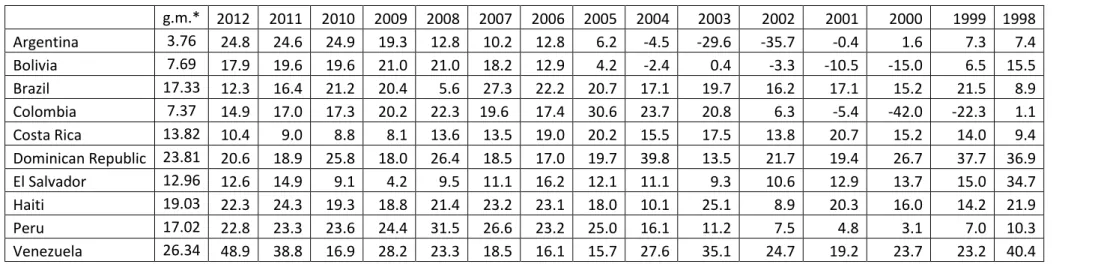
When looking at the whole period of 1998-2012 we see that Venezuelan banks appear to be the most profitable. Their ROE geometric mean for annual returns is 26.34%. Argentinian banks are the least profitable with ROE geometric mean of 3.76%.

(21)

19

Table IV. Return on Assets (*100%).

g.m.* 2012 2011 2010 2009 2008 2007 2006 2005 2004 2003 2002 2001 2000 1999 1998 Argentina 0.47 2.50 2.55 2.72 2.14 1.40 1.14 1.42 0.65 -0.46 -3.50 -4.53 -0.04 0.15 0.61 0.64 Bolivia 0.71 1.45 1.64 1.64 1.85 1.87 1.70 1.31 0.44 -0.25 0.04 -0.33 -1.04 -1.44 0.59 1.27 Brazil 1.64 1.04 1.45 1.93 1.92 0.54 2.61 2.34 2.15 1.72 1.83 1.56 1.61 1.37 1.84 0.68 Colombia 0.87 1.90 2.15 2.14 2.31 2.27 0.90 1.87 3.48 2.65 2.33 0.73 -0.64 -5.38 -3.37 0.18 Costa Rica 1.63 1.49 1.28 1.21 1.07 1.73 1.66 2.31 2.39 1.95 2.31 1.64 2.51 1.23 1.09 0.63 Dominican Republic 2.77 2.11 1.86 2.47 1.75 2.66 2.06 1.98 2.27 4.70 1.76 3.05 2.68 3.14 4.77 4.37 El Salvador 1.34 1.91 2.20 1.27 0.55 1.18 1.32 1.81 1.21 1.05 0.83 0.91 1.10 1.14 1.14 2.56 Haiti 1.26 1.80 1.68 1.38 1.33 1.49 1.71 1.61 1.04 0.51 1.38 0.53 1.24 0.94 0.90 1.34 Peru 1.63 2.25 2.35 2.40 2.28 2.66 2.45 2.21 2.47 1.67 1.03 0.68 0.43 0.27 0.58 0.84 Venezuela 3.51 4.19 3.38 1.87 3.31 2.94 2.63 2.80 3.49 5.52 5.08 3.49 2.57 3.10 3.03 5.30

Source: Bankscope. *geometric mean for the 1998-2012 period.

Table V. Return on Equity (*100%).

g.m.* 2012 2011 2010 2009 2008 2007 2006 2005 2004 2003 2002 2001 2000 1999 1998 Argentina 3.76 24.8 24.6 24.9 19.3 12.8 10.2 12.8 6.2 -4.5 -29.6 -35.7 -0.4 1.6 7.3 7.4 Bolivia 7.69 17.9 19.6 19.6 21.0 21.0 18.2 12.9 4.2 -2.4 0.4 -3.3 -10.5 -15.0 6.5 15.5 Brazil 17.33 12.3 16.4 21.2 20.4 5.6 27.3 22.2 20.7 17.1 19.7 16.2 17.1 15.2 21.5 8.9 Colombia 7.37 14.9 17.0 17.3 20.2 22.3 19.6 17.4 30.6 23.7 20.8 6.3 -5.4 -42.0 -22.3 1.1 Costa Rica 13.82 10.4 9.0 8.8 8.1 13.6 13.5 19.0 20.2 15.5 17.5 13.8 20.7 15.2 14.0 9.4 Dominican Republic 23.81 20.6 18.9 25.8 18.0 26.4 18.5 17.0 19.7 39.8 13.5 21.7 19.4 26.7 37.7 36.9 El Salvador 12.96 12.6 14.9 9.1 4.2 9.5 11.1 16.2 12.1 11.1 9.3 10.6 12.9 13.7 15.0 34.7 Haiti 19.03 22.3 24.3 19.3 18.8 21.4 23.2 23.1 18.0 10.1 25.1 8.9 20.3 16.0 14.2 21.9 Peru 17.02 22.8 23.3 23.6 24.4 31.5 26.6 23.2 25.0 16.1 11.2 7.5 4.8 3.1 7.0 10.3 Venezuela 26.34 48.9 38.8 16.9 28.2 23.3 18.5 16.1 15.7 27.6 35.1 24.7 19.2 23.7 23.2 40.4

(22)

20

Source: author’s calculations in Stata 11 software program.

4. Empirical Results

The purpose of our estimations is to investigate how bank efficiency, bank market concentration and bank profitability affect economic growth in Latin America. We have got a panel dataset for 10 Latin American countries for the time period from year 1998 till year 2012. Bank efficiency is estimated via data envelopment analysis technique; bank market concentration is measured by Herfindahl-Hirschman Index; ROA and ROE ratios are included in the dataset as measures of bank profitability. Dependent variables to represent economic growth are GDP, gross fixed capital formation, household final consumption expenditure, and imports and exports of goods and services.

We perform Levin-Lin-Chu panel unit root test for our panel data. The test assumes that each individual unit in the panel shares the same first order autoregressive (AR(1)) coefficient, but allows for individual effects, time effects and a time trend. The null hypothesis proposes the existence of non-stationarity. The test results are presented in Table V. The null hypothesis is rejected for all the tested variables.

Table V. Levin-Lin-Chu panel unit root test.

Variables coefficient t-star P > t

First difference of the natural logarithm of the GDP -1.1096 -11.3930 0.0000 First difference of the natural logarithm of the

household final consumption expenditure -1.0285 -9.8463 0.0000 First difference of the natural logarithm of the gross

fixed capital formation -1.0307 -10.7212 0.0000 First difference of the natural logarithm of the exports -1.0980 -9.3566 0.0000 First difference of the natural logarithm of the imports -0.9685 -7.9337 0.0000 Natural logarithm of DEA bank cost efficiency -0.3105 -3.6661 0.0001 Natural logarithm of DEA bank market concentration

measure (HHI) -0.4587 -4.8435 0.0000 Return on assets ratio (ROA) -0.4489 -3.4503 0.0003 Return on equity ratio (ROE) -0.4122 -3.1867 0.0007

(23)

21

There are two common assumptions made about the individual specific effects in a panel dataset: the random effects assumption and the fixed effects assumption. The random effects assumption (made in a random effects model) implies that the individual specific effects are uncorrelated with the independent variables. The fixed effect assumption implies that the individual specific effects are correlated with the independent variables. Hausman test is used to differentiate between fixed effects model and random effects model in panel data. In this test random effects model is preferred under the null hypothesis due to higher efficiency, while under the alternative fixed effects model is at least consistent and thus preferred. Hausman test applied to all the dependent variables in our dataset favours the random effects model as the test’s null hypothesis is not rejected. The Breusch and Pagan Lagrangian multiplier (LM) test helps us to decide between a random effects regression and a simple ordinary least squares (OLS) regression. The null hypothesis in the LM test states that variances across units are zero. That is, no significant difference across countries does exist (i.e. no panel effect). The null hypothesis of the LM test is rejected for our dataset, and it justifies the selection of random effects model.

Fortunately, this method allows us to carry out research for dataset with relatively few observations6. Totally we estimate 10 regressions in this paper. The results can be found in Appendix A (Tables from A1 to A5). There are 5 dependent variables that were tested: gross domestic product, gross fixed capital formation, household final consumption expenditure, exports and imports of goods and services. For each dependent variable there are 2 regressions that have a common set of independent variables (lag1 of the independent variable, DEA bank

6

For example we have 150 observations for each of the response variables by bringing together values for 10 countries during the 15 years period.

(24)

22

cost efficiency, HHI), and they differ by the presence of either ROA or ROE in the dependent variables list.

Relatively high values of squared residuals allow us to accept the validity of the estimation results. Tables from VI to X list the effects of the explanatory variables and their statistical significance.

Table VI. Summary of the estimation results for Gross Domestic Product.

Regression 1 Regression 2

Explanatory Variables Effect Explanatory Variables Effect

Lag1 GDP + *** Lag1 GDP + *** Bank cost efficiency - Bank cost efficiency - Bank market concentration

measure (HHI) -

Bank market concentration measure (HHI) - Return on Assets ratio (ROA) + * Return on Equity ratio (ROE) + *** Constant + Constant +

+Positive effect; - Negative effect. * Statistically significant at 10%; ** statistically significant at 5%; *** statistically significant at 1%.

Source: Estimation results of equation (1) reported in Table A1 of Appendix A.

Table VII. Summary of the estimation results for Gross Fixed Capital Formation.

Lag1 Gross fixed capital

formation + ***

Lag1 Gross fixed capital

formation + *** Bank cost efficiency - Bank cost efficiency - Bank market concentration

measure (HHI) -

Bank market concentration measure (HHI) - Return on Assets ratio (ROA) + *** Return on Equity ratio (ROE) + *** Constant + Constant +

(25)

23

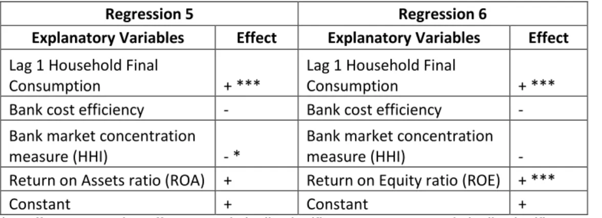
Table VIII. Summary of the estimation results for Household Final Consumption Expenditure.

Lag 1 Household Final

Consumption + ***

Lag 1 Household Final

Consumption + *** Bank cost efficiency - Bank cost efficiency - Bank market concentration

measure (HHI) - *

Bank market concentration measure (HHI) - Return on Assets ratio (ROA) + Return on Equity ratio (ROE) + *** Constant + Constant +

Table IX. Summary of the estimation results for Exports of Goods and Services.

Lag1 Exports + *** Lag1 Exports + *** Bank cost efficiency - Bank cost efficiency - Bank market concentration

measure (HHI) -

Bank market concentration measure (HHI) - Return on Assets ratio

(ROA) + ***

Return on Equity ratio

(ROE) + *** Constant + Constant +

Table X. Summary of the estimation results for Imports of Goods and Services.

Lag1 Imports + *** Lag1 Imports + *** Bank cost efficiency - Bank cost efficiency - Bank market concentration

measure (HHI) -

Bank market concentration measure (HHI) - Return on Assets ratio

(ROA) + *** Return on Equity ratio (ROE) + ** Constant + Constant +

(26)

24

When comparing the estimated models we see that the effects of the explanatory variables across the regressions are equal in terms of their sign and slightly different in terms of their statistical significance.

In all the cases the first lags of the response variables positively contribute to their variation.

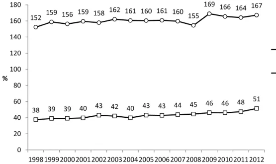
Bank cost efficiency appears to be statistically insignificant in all the regressions. One of the reasons for this can be relatively small contribution of the financial sector of these countries to economic growth. In Figure 2 we can see that the economies in the Latin American countries are not very ‘credit-driven’ when compared to the world economy. The average value for domestic credit provided by financial sector as a percentage of GDP for the 10 Latin American countries which we look at in this paper is 43% throughout the 1998-2012 period. In contrast the same value for the world economy is 161%.

Figure 2. Domestic credit provided by financial sector as a percentage of GDP.

Source: World Bank.

38 39 39 40 43 42 40 43 43 44 45 46 46 48 51 152 159 156 159 158 162 161 160 161 160 155 169 166 164 167 0 20 40 60 80 100 120 140 160 180 199819992000200120022003200420052006200720082009201020112012 % SAMPLE AVERAGE World

(27)

25

Bank market concentration mainly is also not statistically significant in our tests. There is a hypothesis that in a less concentrated market competition compels banks to be more efficient and as a consequence to contribute more to economic growth. However the study by Chortareas et al. (2012) shows that market concentration has no influence on bank efficiency in Latin American countries. Hence we consider that this argument explains the absence of statistically significant evidence of correlation between bank market concentration and economic growth.

ROE and ROA ratios positively influence all the dependent variables and are statistically significant in almost all the cases. This evidence tells us that bank profitability goes in line with economic growth.

We also apply the same model for a sample that excludes Brazil. Brazil is the largest economy among Latin American countries. Its share in the economy of Latin American region averages around 30%, and around 60% in our sample of 10 selected countries. We come up with the same results as described above: no statistically significant effect of bank efficiency and bank market concentration on GDP and its components. Bank profitability ratios still have statistically significant positive effects on economic growth of the countries.

5. Summary and Conclusions

In contrast to the academic studies which investigate relationship between indicators of financial development such as credit to GDP ratios, monetary aggregates, stock exchange market capitalization et cetera, and economic growth, our paper examines the effects of bank efficiency, bank market concentration and bank profitability on GDP and its components. We focus on the economic

(28)

26

performance of 10 Latin American countries between year 1998 and year 2012, that is to say, time that follows the financial liberalization period of early 1990s and covers 2 recession periods for the world economy.

Bank cost efficiency is estimated by Data Envelopment Analysis and bank market concentration is measured by Herfindahl-Hirschman Index. These variables along with the return on assets and return on equity ratios are used to perform panel data regression analysis where Gross Domestic Product and its components are dependent variables.

The dataset is represented by a panel that covers consolidated accounts of commercial, savings and investment banks of 10 Latin American countries: Argentina, Bolivia, Brazil, Colombia, Costa Rica, Dominican Republic, El Salvador, Haiti, Peru and Venezuela.

Our results show that in the framework of our model the influence of bank efficiency and bank market concentration on economic growth is not significant. The same results are obtained when Brazil is excluded out of the sample. However the bank performance variables represented by ROA and ROE ratios confirm that bank returns are in line with changes in economic growth both for whole sample regressions and for the ‘without Brazil’ sample regressions.

Further research on this topic can involve other techniques for measuring bank cost efficiency and bank market concentration in order to use them as variables to explain economic growth in Latin American countries. Analysis that considers the countries on the individual level or on the industry level can be executed as well.

(29)

27

References

Aghion, P., Howitt, P. & Mayer-Foulkes, D. (2005). The effect of financial development on convergence: Theory and evidence. Quarterly Journal of Economics 120,173–222. Al-Awad, M., & Harb, N. (2005). Financial development and economic growth in the Middle East. Applied Financial Economics 15,1041–51.

Andersen, T., & Tarp, F. (2003). Financial liberalization, financial development and economic growth in LDCs. Journal of International Development 15,189–209.

Beck, T. (2002). Financial development and international trade: Is there a link? Journal of

International Economics 57,107–31.

Beck, T., Demirgüç-Kunt, A., & Levine R. (2004). Finance, Inequality and Poverty: Cross-Country Evidence. World Bank Policy Research Working Papers No. 3338.

Beck, T., Levine, R. & Loayza, N. (2000). Finance and the sources of growth. Journal of

Financial Economics 58, 261–300.

Benhabib, J. & Spiegel M. (2000). The role of financial development in growth and investment. Journal of Economic Growth 5, 341–60.

Berthélemy, JC., & Varoudakis, A. (1996). Economic growth, convergence clubs, and the role of financial development. Oxford Economic Papers 48,300–28.

Blanco, L. (2009). The finance-growth link in Latin America. Southern Economic Journal

76(1), 224-248.

Blanco, L. (2013). Finance, growth and institutions in Latin America: What are the links?

Latin American Journal of Economics 50 (2), 179-208.

Calderón, C. & L. Liu (2003). The direction of causality between financial development and economic growth. Journal of Development Economics 72, 321–34.

Cetorelli, N. & Gambera, M. (2001). Banking market structure, financial dependence and growth: international evidence from industry data. Journal of Finance 56, 617-648. Chortareas, G.E., Garza-Garcia, J.G., & Girardone, C. (2010). Banking sector

performance in some Latin American countries: Market power versus efficiency. Banco de

México Working Papers No. 2010-20.

Chortareas, G. E., Garza-Garcia, J.G., & Girardone, C. (2012). Competition, efficiency and interest rate margins in Latin American banking. International Review of Financial

Analysis 24, 93-103.

Claessens, S. & L. Laeven (2004). What drives bank competition? Some international evidence. Journal of Money, Credit, and Banking 36, 563-583

Claessens, S. & Laeven, L. (2005).Financial dependence, banking sector competition, and economic growth. Journal of the European Economic Association 3 (1), 179-207. Claessens, S., Demirgüç-Kunt, A., Huizinga, H. (2001). How does foreign entry affect domestic banking markets? Journal of Banking and Finance 25 (5), 891-912.

Coelli, T. J., Prasada Rao D.S., O’Donnell C.J., & Battese G.E. (2005) Data Envelopment Analysis. An Introduction to Efficiency and Productivity Analysis, 161-181.

De Gregorio, J., & Guidotti, P. (1995). Financial development and economic growth.

World Development 23,433–48.

Demetriades, P., & Hussein, K. (1996). Does financial development cause economic growth? Time series evidence from 16 countries. Journal of Development Economics 51,387–411.

(30)

28

Demirgüç-Kunt, A. (2006). Finance and economic development: Policy choices for developing countries. World Bank Policy Research, WP 3955

Denizer, C.A., Dinç, M., & Tarimcilar, M. (2000). Financial liberalization and banking efficiency: Evidence from Turkey. Journal of Productivity Analysis 27 (3), 177-195. Ferreira, C. (2012). Bank efficiency, market concentration and economic growth in the European Union. ISEG Working Papers, WP 38/2012DE/UECE.

Galindo, A., Micco, A., & Panizza, U. (2006). Two decades of financial reforms. In: Lora E.

The state of state reform in Latin America, Washington: Inter-American Development

bank, 291-316.

Greenwood, J., & Jovanovic B. (1990). Financial development, growth, and the distribution of income. Journal of Political Economy 98,1076–1107.

Habibullah, M., & Eng, Y.K. (2006). Does financial development cause economic growth? A panel data dynamic analysis for the Asian developing countries. Journal of the Asia

Pacific Economy 11,377–93.

Hermes, N., & Lensink, R. (2005). Does financial liberalization influence saving,

investment and economic growth? Evidence from 25 emerging market economies, 1973-96. UNU-WIDER, United Nations University Research Paper No. 2005/69.

Hermes, N., & Nhung, V.T.H. (2010). The impact of financial liberalization on bank

efficiency: evidence from Latin America and Asia. Applied Economics 42(26), 3351-3365. Herrero A.G., Gallego J.S.S., Cuadro L. & Egea C. (2002). Latin American financial development in perspective. Banco de España, Servicio de Estudios, Documento de

Trabajo 0216.

Iyare, S., Lorde, T., & Francis, B. (2005). Financial development and economic growth in developing economies: Empirical evidence from the Caribbean. Ekonomia 8,168–84. Jung, W. (1986). Financial development and economic growth: International evidence.

Economic Development and Cultural Change 34,333–46.

Kaminsky, G., & Schmukler, S. (2003). Short-run pain, long-run gain: the effects of financial liberalization. National Bureau of Economic Research, WP 9787.

Khan, M. & Senhadji, A. (2003). Financial development and economic growth: A review and new evidence. Journal of African Economies 12,89–110.

King, R. & Levine, R. (1993) Finance and Growth: Schumpeter Might be Right. Quarterly

Journal of Economics 108 (3), 717-737.

Kroszner, R., Laeven, L. & Klingebiel, D. (2007). Banking crisis, financial dependence and growth. Journal of Financial Economics 84,187–228.

Levine, R. (1997). Financial development and economic growth: Views and agenda.

Journal of Economic Literature 35, 688-726.

Levine, R. (2005). Finance and growth: Theory and evidence. In: Aghion P. and Durlauf S. Handbook of economic growth, North-Holland: Elsevier, pp. 866–934.

Loayza, N., & Ranciere R. (2006). Financial development, financial fragility, and growth.

Journal of Money, Credit, and Banking 38, 1051–76.

Love, I. (2003). Financial development and financing constraints: International evidence from the structural investment model. Review of Financial Studies 16,765–91.

Luintel, K. & M. Khan (1999). A quantitative reassessment of the finance-growth nexus: Evidence from a multivariate VAR. Journal of Development Economics 60, 381–405.

(31)

29

Manning, M. (2003). Finance causes growth: Can we be so sure? Contributions to

Macroeconomics 3,12.

Maudos, J. & Fernandez de Guevara, J. (2006). Banking competition, financial dependence and economic growth. Munich Personal RePEc Archive, MPRA paper 15254.

Naceur, S., & Ghazouani, S. (2007). Stock markets, banks, and economic growth: Empirical evidence from the MENA region. Research in International Business and

Finance 21,297–315.

Nourzad, F. (2002). Financial development and productive efficiency: A panel study of developed and developing countries. Journal of Economics and Finance 26, 138–49. Odhiambo, N. (2007). Supply-leading versus demand-following hypothesis: Empirical evidence from three SSA countries. African Development Review 19,257–80.

Rajan, R. & Zingales, L. (1998). Financial dependence and growth. American Economic

Review 88, 559-587.

Ram, R. (1999). Financial development and economic growth: Additional evidence.

Journal of Development Studies 35, 164–74.

Rioja, F. & Valev, N. (2004a). Finance and the sources of growth at various stages of economic development. Economic Inquiry 42, 127–40.

Rioja, F. & Valev, N. (2004b). Does one size fit all? A reexamination of the finance and growth relationship. Journal of Development Economics 74, 429–47.

Shan, J. (2005). Does financial development ‘lead’ economic growth? A vector auto-regression appraisal. Applied Economics 37, 1353–67.

Shan, J., Morris, A. & Sun, F. (2001). Financial development and economic growth: An egg-and-chicken problem? Review of International Economics 9, 443–54.

Shen, C.H., & Lee C.C. (2006). Same financial development yet different economic growth—Why? Journal of Money, Credit and Banking 38,1907–44.

Thanassoulis, E., Portela, M.C.S. & Despic, O. (2008). DEA – The Mathematical

Programming Approach to Efficiency Analysis. In: Fried, H.O., Lovell, C.A.K. & Schmidt, S.S. The measurement of productive efficiency and productivity growth, New York: Oxford University Press, pp. 251-420.

Weill, L. (2004). Measuring cost efficiency in European banking: a comparison of frontier techniques. Journal of Productivity Analysis 21-2, 133-152.

Xu, Z. (2000). Financial development, investment, and economic growth. Economic

Inquiry 38,331–44.

Yeyati, E.L., & Micco, A. (2003). Banking Competition in Latin America. Latin American

(32)

30

Appendix A. Estimation results.

Table A1. Regressions for Gross Domestic Product.

logGDP coef std err Z P>|z| logGDP Coef Std Err Z P>|z|

lag1logGDP 0.994 0.010 96.91 0.000 lag1logGDP 0.992411 0.010457 94.9 0.000 logTE -0.015 0.029 -0.51 0.610 logTE -0.03052 0.029799 -1.02 0.306 logHHI -0.068 0.153 -0.44 0.658 logHHI -0.07484 0.156736 -0.48 0.633 ROA 0.033 0.009 3.67 0.000 ROE 0.00367 0.001081 3.4 0.001 constant 0.268 0.431 0.62 0.535 constant 0.432016 0.437599 0.99 0.324 R-squared 0.9924 R-squared 0.9923 Number of observations 140 Number of observations 140

Table A2. Regressions for Gross Fixed Capital Formation.

logGFCF Coef Std Err Z P>|z| logGFCF Coef Std Err Z P>|z|

lag1logGFCF 0.9924 0.0105 94.90 0.000 lag1logGFCF 0.9859 0.0147 66.91 0.000 logTE -0.0305 0.0298 -1.02 0.306 logTE -0.0289 0.0420 -0.69 0.490 logHHI -0.0748 0.1567 -0.48 0.633 logHHI -0.3314 0.2221 -1.49 0.136 ROA 0.0037 0.0011 3.40 0.001 ROE 0.0479 0.0130 3.69 0.000 constant 0.4320 0.4376 0.99 0.324 constant 0.5165 0.5906 0.87 0.382 R-squared 0.9841 R-squared 0.9842 Number of observations 140 Number of observations 140

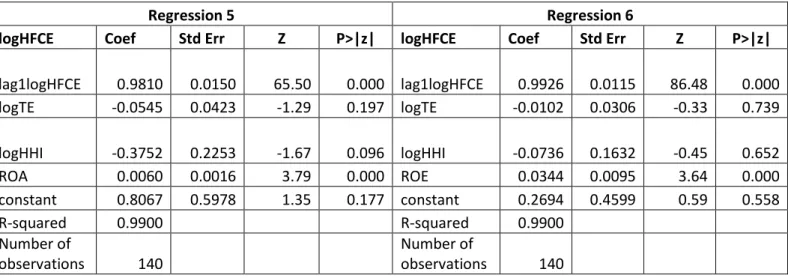
Table A3. Regressions for Household Final Consumption Expenditure.

logHFCE Coef Std Err Z P>|z| logHFCE Coef Std Err Z P>|z|

lag1logHFCE 0.9810 0.0150 65.50 0.000 lag1logHFCE 0.9926 0.0115 86.48 0.000 logTE -0.0545 0.0423 -1.29 0.197 logTE -0.0102 0.0306 -0.33 0.739 logHHI -0.3752 0.2253 -1.67 0.096 logHHI -0.0736 0.1632 -0.45 0.652 ROA 0.0060 0.0016 3.79 0.000 ROE 0.0344 0.0095 3.64 0.000 constant 0.8067 0.5978 1.35 0.177 constant 0.2694 0.4599 0.59 0.558 R-squared 0.9900 R-squared 0.9900 Number of observations 140 Number of observations 140

(33)

31

Table A4. Regressions for Exports of Goods and Services.

logEXP Coef Std Err Z P>|z| logEXP Coef Std Err Z P>|z|

lag1logEXP 0.9894 0.0116 85.01 0.000 lag1logEXP 0.9715 0.0164 59.27 0.000 logTE -0.0275 0.0308 -0.89 0.371 logTE -0.0466 0.0431 -1.08 0.280 logHHI -0.0950 0.1660 -0.57 0.567 logHHI -0.2767 0.2168 -1.28 0.202 ROA 0.0041 0.0011 3.59 0.000 ROE 0.0364 0.0123 2.97 0.003 constant 0.4681 0.4641 1.01 0.313 constant 0.9919 0.6482 1.53 0.126 R-squared 0.9841 R-squared 0.9836 Number of observations 140 Number of observations 140

Table A5. Regressions for Imports of Goods and Services.

logIMP Coef Std Err Z P>|z| logIMP Coef Std Err Z P>|z|

lag1logIMP 0.9742 0.0167 58.44 0.000 lag1logIMP 0.9822 0.0142 68.96 0.000 logTE -0.0552 0.0441 -1.25 0.211 logTE -0.0321 0.0371 -0.87 0.386 logHHI -0.2154 0.2223 -0.97 0.333 logHHI -0.1369 0.1913 -0.72 0.474 ROA 0.0031 0.0015 2.08 0.038 ROE 0.0333 0.0110 3.04 0.002 constant 1.0091 0.6624 1.52 0.128 constant 0.6582 0.5562 1.18 0.237 R-squared 0.9871 R-squared 0.9867 Number of observations 140 Number of observations 140