Discrete and continuous SIS epidemic models: a unifying approach

Discrete and continuous SIS epidemic models: a

unifying approach

Fabio A. C. C. Chaluba_{, Max O. Souza}b,∗

a

Departamento de Matem´atica and Centro de Matem´atica e Aplica¸c˜oes, Universidade Nova de Lisboa, Quinta da Torre, 2829-516, Caparica, Portugal.

b

Departamento de Matem´atica Aplicada, Universidade Federal Fluminense, R. M´ario Santos Braga, s/n, 22240-920, Niter´oi, RJ, Brasil.

Abstract

The Susceptible-Infective-Susceptible (SIS) epidemiological scheme is the simplest description of the dynamics of a disease that is contact-transmitted, and that does not lead to immunity. Two by now classical approaches to such a description are: (i) the use of a mass-action compartamental model that leads to a single ordinary differential equation (SIS-ODE); (ii) the use of a discrete-time Markov chain model (SIS-DTMC). While the former can be seen as a mean-field approximation of the latter under certain conditions, it is also known that their dynamics can be significantly different, if the ba-sic reproduction number is greater than one. The goal of this work is to introduce a continuous model, based on a partial differential equation (SIS-PDE), that retains the finite populations effects present in the SIS-DTMC model, and that allows the use of analytical techniques for its study. In par-ticular, it will reduce itself to the SIS-ODE model in many circumstances. This is accomplished by deriving a diffusion-drift approximation to the prob-ability density of the SIS-DTMC model. Such a diffusion is degenerated at the origin, and must conserve probability. These two features then lead to an interesting consequence: the biologically correct solution is a measure solution. We then provide a convenient representation of such a measure solution that allows the use of classical techniques for its computation, and that also provides a tool for obtaining information about several dynamical features of the model. In particular, we show that the SIS-ODE gives the most likely state, conditional on non-absorption. As a further application of

such representation, we show how to define the disease-outbreak probability in terms of the SIS-PDE model, and show that this definition can be used both for certain and uncertain initial presence of infected individuals. As a final application, we compute an approximation for the extinction time of the disease. In addition, we present many numerical examples that confirm the good approximation of the SIS-DTMC by the SIS-PDE.

Keywords: SIS Epidemiological Models, IBM Modelling, Differential Equations, Diffusive Limits

1. Introduction

Real populations are always finite. This means that stochastic effects will, sooner or later, play a significant role on its development. However, in very large populations the time scale for such stochastic events can be extremely long and, in these cases, the dynamics may be well approximated by a deterministic model. In the realm of epidemiological models, such course led to the development of compartmental mass action models pioneered by MacDonald and Ross (see Ross, 1911; Macdonald, 1957). This in turn sprung into a development of its own, benefited by the powerful analytical results in differential equations and dynamical systems (Anderson and May, 1995; Diekmann et al., 2013).

Nevertheless, there are many cases where stochastic effects cannot be neglected: moderately large populations or low population variability Ross (2011). These situations naturally led to the development of stochastic mod-els for discrete populations with either continuous or discrete time (Allen, 2008; Keeling and Ross, 2008).

As it might be expected, these two paradigms do not, in general, give the same qualitatively dynamics—cf. discussion in §1.1. The very natural question then is how to reconcile such models, or at least to have some criteria for choosing the most appropriate paradigm in a given situation. In general, the answer for this question will be largely dependent on the underlying models.

probabil-ity proportional to the number of infected and to the time of exposure; the IS transition (recovery) occurs with constant-in-time transition probability. This model is summarised in the following diagram:

S+I →β I+I;

I →α S. (1)

The constants α and β in (1) can be interpreted as rates (either discrete or continuous) or as probabilities among many other possible choices. Here, we shall focus on two classical implementations of such dynamics: the first one, based on the mass-action principle and ordinary differential equations ODE), and the second one based on discrete time Markov chains (SIS-DTMC). The former model includes the usual mass-action homogeneity and infinity population assumptions, whereas the SIS-DTMC requires only ho-mogeneity — see the review in §1.1. Although the aim of this work is to understand the models just discussed on a unified framework, it is fair to observe that, in many situations, the heterogeneities of the population can be larger than the ones allowed by these classical models. In this case, alter-natives approaches are necessary. See Diekmann et al. (2013) for a general discussion. In the deterministic framework, there are extensions to account for such heterogeneities as meta-population and multi-group models (e.g. Hyman and Li (1997); Feng et al. (2005); Guo et al. (2006)) or the consid-eration of self-awareness—cf. Van Segbroeck et al. (2010). In the stochastic framework, the inner variability of individuals can lead to non-Markovian dynamics as statistically observed in Yang (1972); Becker (1989) and this motivated the development of corresponding non-Markov models Mieghem (2013); Cator et al. (2013).

In connection with these two classical models, our main aim is to intro-duce a continuous model that will approximate the stochastic model, in the large population regime, but that will also approximate the deterministic model in many circumstances. In particular, it will honour its qualitatively dynamics of the stochastic model, but it will also reduces to the deterministic one when both dynamics are compatible. As a consequence, this continuous model provides a unifying view of both formulations, and it also brings for-ward the tools of differential equations to contribute for their analysis.

1.1. Classical discrete and continuous views of the SIS model

dis-cussed in many classical and more recent references (see, e.g, Rass and Rad-cliffe (2003); Bailey (1975); Dietz (1975); Anderson and May (1995); Diek-mann et al. (2013)), and it is given by the following system of ODEs:

˙

S = −αSI+βI

˙

I = αSI−βI .

Assuming, without loss of generality, that S(0) +I(0) = 1, we find

I′ =αI

1− β

α −I

. (2)

The final value as int→ ∞of the solution for any non-trivial initial condition depends on the value R0 := α/β. For R0 ≤ 1, this limiting value is zero— the so-called disease free equilibrium; otherwise it is is a positive constant

I∗ = 1−R−01—the endemic equilibrium.

The second approach, the SIS-DTMC, consists of a population ofN indi-viduals, divided in two subgroups: N x Infected and N(1−x) Susceptibles, where x ∈ {0,_N1,_N2, . . . ,1} is the fraction of infected. At each time step ∆t >0 one individual is chosen at random and then

• If it is of type I, then it becomes S with probability β;

• If it is of typeS, then it becomesIwith probability proportional to the number of infected in the population: αx.

These rules specify a birth-death process, with the corresponding transition probabilities given by:

T+_{(x) =αx(1−x) ,}

T0(x) = 1−T+(x)−T−(x) , T−(x) =xβ .

Let P(N,∆t)(x, t) be the probability to find a fraction x of I individuals at time t in a population of size N, evolving in time steps of size ∆t. The corresponding master equation is

P(N,∆t)(x, t+ ∆t) =T+(x−z)P(N,∆t)(x−z, t) +T0(x)P(N,∆t)(x, t)+ (3)

T−_(x+z)P

where, for notation convenience, we set z = N−1_{. The state x = 0 is an} absorbing state, and for any choice of β, α > 0, the chain is irreducible. Hence absorption is eventually certain, and thusx= 0 is the only stationary state (see, e.g, Allen (2008)).

In addition, notice that we always have 1

X

x=0

P(N,∆t)(x, t) =

1

X

x=0

P(N,∆t)(x,0) (4)

The master equation (3) can be related with a discrete version of (2) as follows: letXt be the fraction of infected individuals at timet. Let us define

the expected fraction of infected individuals:

n(t) = E_{[Xt] =}

1

X

x=0

xP(N,∆t)(x, t) ,

Therefore

n(t+ ∆t) = 1

X

x=0

xα(x−z)(1−x+z)P(N,∆t)(x−z, t)

+ 1

X

x=0

x(1−αx(1−x)−βx)P(N,∆t)(x, t)

+ 1

X

x=0

xβ(x+z)P(N,∆t)(x+z, t)

= 1

X

x=0

(x+z)αx(1−x)P(N,∆t)(x, t)

+ 1

X

x=0

x(1−αx(1−x)−βx)P(N,∆t)(x, t)

+ 1

X

x=0

(x−z)βxP(N,∆t)(x, t)

= 1

X

x=0

xP(N,∆t)(x, t) +z(α−β)

1

X

x=0

xP(N,∆t)(x, t)−zα

1

X

x=0

x2P(x, t)

=

1 + α

N

1− 1

R∗

0

n(t)− α

N

1

X

x=0

x2_P

(N,∆t)(x, t)

=n(t) + α

Nn(t)

1− 1

R∗

0

−n(t)

− α

NV[Xt],

whereV_{denotes the variance andR0}∗ _{=α/β. Then, if we letα/N = ∆t, and}

neglect the variance term, we are left with an Euler discretisation of (2). No-tice, however, that neglecting the variance term is not justifiable close to the disease extinction or to the endemic equilibrium. For a comprehensive mono-graph about the SIS DTMC, see N˚asell (2011). See also Bailey (1963); Allen (1994); Allen and Burgin (2000); Allen (2008); McKane and Newman (2004) and references therein for different interpretations of stochastic modelling in epidemiology. See also Allen (1994) for discrete deterministic versions of epi-demiological models, and a discussion where chaotic behaviour can appear and depart significantly from the corresponding continuous model.

results obtained might differ considerably. In particular, as discussed be-fore, for certain choices of parameters, there is a non-trivial stationary solu-tion, which attracts all non-trivial initial conditions of the SIS-ODE model, whereas for the SIS-DTMC model, the only stationary state is the trivial one.

This apparent contradiction is solved by considering the behaviour of the transient states of the discrete process in the limit of large population. In-deed, the SIS-DTMC model is a Markov chain with leading eigenvalueλ= 1; the associated eigenvector denotes the trivial state, the only stationary state of the process and the absorbing state of any initial condition. The second eigenvalueλ∗ ∈(0,1) is associated to the transient state and the typical time

such that the transient state fades out is directly related to the inverse size of the spectral gap 1−λ∗. However, when the population is large 1−λ∗ ≪1,

making the transient state a quasi-stationary one. See N˚asell (2011). There-fore, in the limit of infinite population (one of the basic assumptions of any modelling by ordinary differential equations) we possibly have a stationary state that is not present in the discrete model. In addition, for initial pop-ulations with a small fraction of infected individuals, the stochastic effects can lead to disease extinction in a much faster time scale.

1.2. Unified modelling

in order to obtain information of the solution of the discrete SIS model. Re-calling that every population is finite, we have a partial differential equation model that gives information on the final and transient states of the discrete problem. Therefore, it generalises the ODE model to all time scales.

The first goal in this work is to derive the first order correction for the continuous model for finite size population effects. This is done in two steps: in the first step, we perform a formal asymptotic expansion in N of the transition matrix. This can be seen as reminiscent of the Kramers-Moyal expansion (Gardiner et al., 1985) or as a system size expansion (van Kampen, 2001), but we follow a more analytical route, along the lines of Chalub and Souza (2009a). Then, we obtain the following PDE:

∂tp=−∂x{x[R0(1−x)−1]p}+

1 2N∂

2

x{x(R0(1−x) + 1)p}, (5)

supplemented with the boundary condition 1

2N ((1−R0)p(1, t) +∂xp(1, t)) +p(1, t) = 0,

and the conservation law d dt

Z 1

0

p(x, t) dt= 0. (6)

When N is equal to infinity, we formally obtain the equation:

∂tp=−∂x{x[R0(1−x)−1]p} , (7)

supplemented by the boundary condition

p(1, t) = 0.

In this case, the conservation law (6) is always satisfied.

Dirac mass at the origin, which means that the disease will be eventually be extinguished.

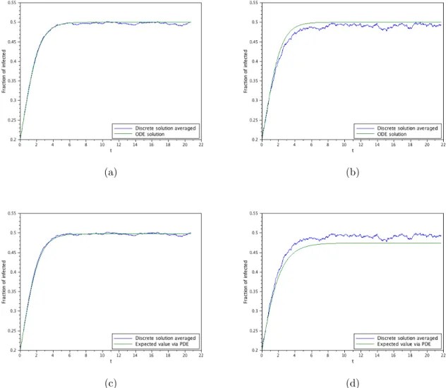
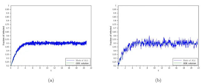
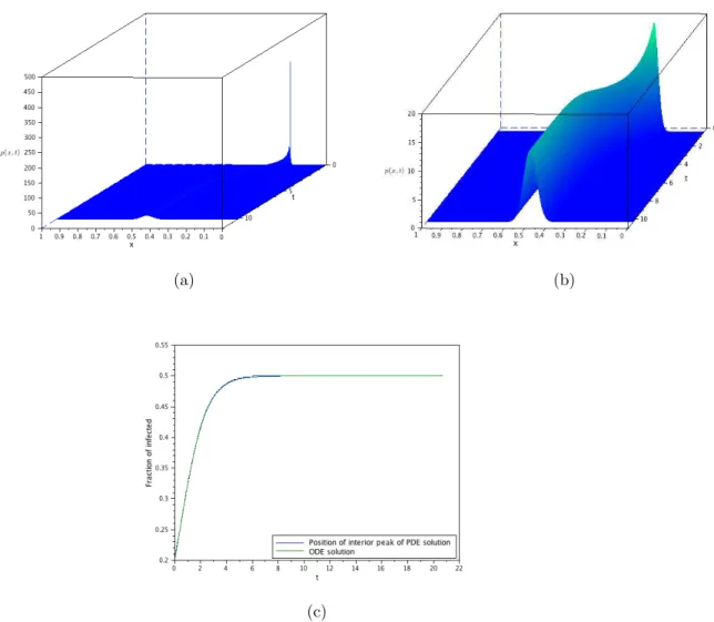
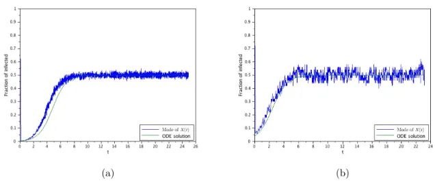
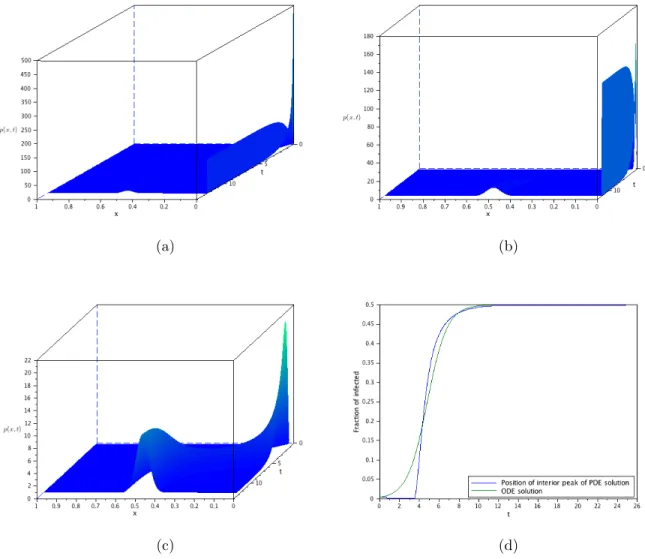
The second goal of this work is to probe the difference between the de-terministic, the stochastic and the diffusion approximation obtained here through numerical simulations of the models. These simulations will con-firm that the SIS-PDE is a consistent approximation of the SIS-DTMC and, consequently, to the SIS-ODE when it agrees with the SIS-DTMC. As a by-product, these simulations will also show that the ODE-SIS formulation models the interior mode (i.e., the mode of the probability distribution re-stricted to x > 0) of the probability distribution, and not the mean value. They will also shown the departure of the SIS-ODE model when the number of infected individuals is small, even if the entire population is large.

The third and final goal is to illustrate how the continuous formulation can contribute to the study of the dynamical features of the SIS-DTMC model. Using the information from the representation of the PDE solution, we give a slightly modified definition of outbreak probability, which agrees with the classical ones when considering the discrete counterpart, and show that the usual approximation—as given in (Allen, 2008)—can incur in serious errors for slightly supercritical values of R0. In particular, we shall consider the outbreak threshold number, T0, recently introduced by Hartfield and Alizon (2013) and see how their results change in view of these differences. Finally, we provide an asymptotic derivation of the extinction time that complements earlier results by N˚asell (2011) and even earlier results by Doering et al. (2005).

1.3. Outline

2. Formal Derivation of PDE model

2.1. Asymptotic expansion

We proceed with a second order Taylor expansion inxofP(N,∆t)and find

P(N,∆t)(x±z, t) =P(N,∆t)(x, t)±z∂xP(N,∆t)(x, t) +

z2 2 ∂

2

xP(N,∆t)(x, t) +O z3

.

(8) Using P =P(N,∆t)(x, t), we derive the formal expansion for equation (3):

P(N,∆t)(x, t+ ∆t) = α(x−z)(1−x+z)

P −z∂xP +

z2 2 ∂

2

xP

+ (1−βx−αx(1−x))P +β(x+z)

P +z∂xP +

z2 2∂

2

xP

+O βz3, αz3

=P +z(−α(1−2x)P −αx(1−x)∂xP +βP +βx∂xP)

+z2

−αP +α(1−2x)∂xP +

αx(1−x)

2 ∂

2

xP +β∂xP +

βx

2 ∂ 2

xP

+O βz3, αz3

=P +z∂x(βxP −αx(1−x)P) +

z2 2∂

2

x(βxP +αx(1−x)P)

+O βz3, αz3

We introduce the following assumptions: 1. β(N,∆t) =β0(∆t)γ(1 + o(∆t)),

2. α(N,∆t)=α0(∆t)γ(1 + o(∆t)). 3. N =κ(∆t)γ−1.

with 0< γ ≤1/2.

For a more detailed discussion about the role of scaling in obtaining the diffusive limit, see Chalub and Souza (2009a, 2013)

We also introduce the basic reproductive factor

R0(1 + o(∆t)) , (9)

with R0 =α0/β0, and we rewrite the master equation as: ∆P

∆t = β

N∆t∂x[x(1−R0(1−x))P] + β

2N2_∆t∂ 2

x(x(R0(1−x) + 1)P)

+O ∆t, N−2

On using the assumptions (and rescaling time t→κt/β0), we find

∂tp=−∂x{x[R0(1−x)−1]p}+

1 2N∂

2

x{x(R0(1−x) + 1)p}+O(∆t) ,

(10) Remark 2.1. The fact the equation (10) can be obtained with various time-scale parameters can be used to increase computational efficiency in the sim-ulations. For instance, consider the traditional diffusive scaling ∆t = (∆x)2, and an alternative scaling with γ = 1/4, hence ∆t = (∆x)4/3. The ratio of the latter to the former is (∆x)−2/3_{, which for N = 200 is approximately 34.}

This means that a simulation that runs in one hour with the diffusive scaling will run in less than two minutes in the alternative scaling.

The first approximation of the SIS model, which is size-independent, is given by the hyperbolic equation (7), and it is equivalent to the ODE (2); namely, the characteristics of equation (7) are solutions of (2).

If we consider the first correction due to finite-size effects, we find the parabolic equation (10), setting the O(∆t) term equal to zero.

2.2. Boundary condition and conservation law

Note that we can, in principle, extend equation (3) to values of x larger than 1. The compactness ofP(N,∆t)is preserved; explicitly, ifP(N,∆t)(x,0) = 0 for any x 6∈ [0,1] then P(N,∆t)(x, t) = 0 for any x 6∈ [0,1], and t > 0 (this

follows from the fact that T−_{(0) =T}+_{(1) = 0). Therefore, in the continuous} limit, it is natural to assume that the solution of of the PDE is such that

p(x, t) = 0 for anyx6∈[0,1] and anyt >0. From the uniform parabolicity of the PDE in any neighbourhood of x = 1, we conclude the continuity of the flow of p around x = 1. We initially write the PDE (10) (with null O(∆t) term) in divergence form:

∂tp=∂x (

ε

2[(R0(1−x) + 1)p−xR0p+x(R0(1−x) + 1)∂xp]

+x[R0(1−x)−1]p

)

,

Imposing the continuity of the flow atx= 1, we conclude that

0 = lim

y→0+

hε

2[(1−R0)p|1+y+∂xp|1+y] +p|1+y

i

= lim

y→0+

hε

2[(1−R0)p|1−y+∂xp|1−y] +p|1−y

i

=hε

2[(1−R0)p|1+∂xp|1] +p|1

i

.

Finally, we observe that the conservation law (4) becomes

Z 1

0

p(x, t) dx=

Z 1

0

p(x,0) dx

which we will write as

d dt

Z 1

0

p(x, t) dx= 0. (11)

3. Analytical results for the continuous model

We begin with the weak formulation introduced in Chalub and Souza (2009b) :

Z ∞

0

Z 1

0

p(x, t)∂tφ(x, t) dxdt

+ ε 2 Z ∞ 0 Z 1 0

p(x, t)x(R0(1−x) + 1)∂_x2φ(x, t) dxdt

+

Z ∞

0

Z 1

0

p(x, t)x(R0(1−x)−1)∂xφ(x, t) dxdt

+

Z 1

0

p(x,0)φ(x,0) dx= 0, (12)

where

φ∈C_c∞([0,1]×[0,∞)).

Since we are going to be interested in solution to (12) in a measure sense, we recall the following result proved in Chalub and Souza (2009b):

Lemma 3.1. Let ν be a Radon measure supported in [0,1]. Then we can write ν =ν0+νi+ν1, where sing supp(ν0)⊂ {0}, sing supp(νi)∈(0,1), and

In what follows, we shall be interested in positive and bounded Radon measures in [0,1], and we shall denote these byBM+([0,1]). See Chalub and Souza (2009b) for more details about the choices of spaces.

In view of Lemma 3.1, we shall write for p0 ∈ BM+([0,1]):

p0 =a0δ0+r0+b0δ1.

We now proceed to study (12) more thoroughly. We begin by observing that (12) is uniformly parabolic on [ξ,1], for any 0< ξ <1. In particular we have the following

Lemma 3.2. Let p∈L∞ _[0,∞);BM+_([0,1])

be a solution to (12). Then

p∈C∞((0,∞);C∞((0,1))) .

Furthermore, p(x, t) =a(t)δ0+r(x, t), where r satisfies:

∂tr =−∂x{x[R0(1−x)−1]r}+

ε

2∂ 2

x{x(R0(1−x) + 1)r},

ε

2((1−R0)r(1, t) +∂xr(1, t)) +r(1, t) = 0 (13)

r(x,0) =r0+b0δ1

Moreover,

a(t) = ε(R0+ 1) 2

Z t

0

r(0, s) ds+a0. (14)

Proof. Firstly, in any (a, b)⊂[0,1], (12) is uniformly parabolic, and the local regularity of p follows from standard arguments—see Lieberman (1996).

In view of Lemma 3.1, we write

p(t, x) =a(t)δ0+r(x, t) +b(t)δ1. (15) Let φ(x, t) = η(t)ϕ(x), with η ∈ C∞

c ((0,∞)) and ϕ ∈ Cc∞((0,1)). Then φ

is an appropriate test fuction, and we have recast (12) in terms of r only. Then the regularity of p implies that r ∈ C∞_((0,∞);C∞_{((0,1))), and that}

Now, let ϕ ∈ C∞

c ([0,1]), then on substituting (15) into (12), and using

the regularity of r to integrate by parts, we obtain

Z ∞

0

a(t)η′(t)ϕ(0) dx dt+

Z ∞

0

b(t)η′(t)ϕ(1) dx dt+

+

Z ∞

0

b(t)η(t)ε 2ϕ

′′_(1)−ϕ′_{(1) dx dt+}

+ε(1 +R0) 2

Z ∞

0

r(t,0)ϕ(0) dt−

−

Z ∞

0

r(1, t) + ε

2((1−R0)r(t,1) +∂xr(1, t))

ϕ(1)η(t) dt+

+ε 2

Z ∞

0

r(1, t)ϕ′(1)η(t) dt = 0.

If we choose ϕ ∈ C∞

c ([0,1]), with ϕ(0) = ϕ(1) = ϕ′(1) = 0 and ϕ′′(1) 6= 0,

we find that

ε

2

Z ∞

0

b(t)η(t)ϕ′′(1) dt = 0.

Hence b(t) = 0 for almost every time.

Now, let us choose ϕ with ϕ(0) 6= 0, and ϕ(1) = ϕ′_{(1) = 0. We then}

conclude that

a(t) = ε(R0+ 1) 2

Z t

0

r(0, s) ds+a0,

which is (14). Now let ϕ(x)≡1. Then we are left with

Z ∞

0

r(1, t) + ε

2((1−R0)r(t,1) +∂xr(1, t))

η(t) dt = 0,

and hence we obtain again the boundary condition in (13). Remark 3.3. Notice that we are still left with

ε

2

Z ∞

0

r(1, t)ϕ′(1)η(t) dt= 0.

This identity is satisfied if we choose ϕ with ϕ′_{(1) = 0. However, in general,}

we need to show that ∂xr(1, t) is uniformly bounded in ε. In this case, the

boundary condition in (13) implies that r(1, t) =O(ε), and hence the above identity is O(ε2_{), which can then be consistently neglected at this truncation}

We now turn back to the classical solution. In the following, we write

F(x) = R0(1−x) + 1, Π(x) = 1− 2

F(x), H(x) =x+ 2

R0 log

F(x)

F(0)

.

Proposition 3.4. There exists a unique solution to (13) with r(x,0) =r0+

b0δ1. Such a solution can be written as

r(x, t) =ω(x)

∞

X

k=1

αkeλktϕk(x), (16)

where

ω(x) = P(x)

xF(x), P(x) = exp(2N H(x)),

ϕ satisfies

ω−1(x) 1

2N∂x(P(x)∂xϕk) =λkϕk, ϕk(0) = ∂xϕk(1) = 0, (17)

with λk<0.

Moreover,

αk = Z 1

0

r(x,0)ϕk(x) dx (18)

In particular, r∈C∞_((0,∞);C∞_{([0,1]))∩C (0,∞);BM}+_([0,1]))

, and

lim

t→∞krk∞= 0.

Finally, if r0, b0 ≥0, then r≥0.

Proof. Let

r(x, t) =ω(x)u(x, t) Then equation (13) becomes

ω(x)∂tu=

1

2N∂x(P(x)∂xu)

u(0, t) = ∂xu(1, t) = 0, (19)

u(x,0) =ω−1_{(x) (r}

0(x) +b0δ1).

in the space of C2 _{functions f that satisfy f(0) =f}′_{(1) = 0, with respect to}

the inner product

(f, g) =

Z 1

0

f(x)g(x)ω(x) dx.

Hence, the associated spectral problem is a Sturm-Liouville problem that is singular—of limit-circle type—at the origin. Thus the eigenfunctions yield a Hilbert basis for L2([0,1]). (cf. Zettl (2005)).

Therefore, the solution to (19) can be represented through the corre-sponding spectral expansion (see Evans (2010); Taylor (1996)), i.e.

u(x, t) =

∞

X

k=1

αkeλktϕk(x), αk = (u(·,0), ϕk), (ϕk, ϕk) = 1. (20)

Thus, the expressions (16) and (18) follows immediately from the relation between r and u.

Finally, if r0, b0 ≥0 then we haveu(x,0)≥0, and since (19) satisfies the strong maximum principle Lieberman (1996), we have thatu≥0, and hence

r ≥0.

The important point about solutions in the sense of (12) is that they satisfy probability conservation as the next result shows

Theorem 3.5. Letp∈L∞ _[0,∞);BM+_([0,1])

be a solution to (12). Then

Z 1

0

p(x, t) dx=

Z 1

0

p0(x) dx,

for almost every time.

Proof. Consider φ(t, x) =η(t), with η ∈ Cc([0,∞)), with η(0) = 1.

Substi-tuting in (12) yields

Z ∞

0

Z 1

0

p(x, t)η′(t) dxdt+

Z 1

0

p(x,0) dx= 0

and the result follows.

Theorem 3.6. Let p0 ∈ BM+([0,1]). Then, equation (12) has a unique

solution p∈L∞ _[0,∞);BM+_([0,1])

. Moreover, we have

p(x, t) =a(t)δ0+r(x, t), a(t) =

ε(R0+ 1) 2

Z t

0

with r ∈C∞_{([0,1]×[0,∞)), and}

lim

t→∞kr(·, t)k∞ = 0

lim

t→∞a(t) = 1.

Proof. Let r be the solution to (13). Then all the statements aboutr follow from Proposition 3.4. Let p be given by (21). Then p(x,0) = p0 and, upon substituting pin (12) and integrating by parts the terms withr, one verifies that pis indeed a solution. The statement about a follows from probability conservation.

Now, let ˜p be another solution to (12). By Lemma 3.2, we can write ˜

p(x, t) = ˜a(t)δ0 + ˜r(x, t), and ˜r satisfies (13). By virtue of Proposition 3.4, we have that r = ˜r. On susbtituting ˜p in (12), we find that ˜a = a. Hence

p= ˜p.

4. Numerical illustrations

In this section, we provide a number of numerical examples of the three models considered so far. The choice of examples have two goals in mind: (i) to highlight the differences between the finite and infinite populations cases; (ii) to illustrate the performance of the approximation by the SIS-PDE, obtained in Section 2, and the use of the representation derived in Section 3.

4.1. The supercritical case with significant initial infection

(a) (b)

(c) (d)

(a) (b)

(a) (b)

(c)

4.2. The supercritical case with a small initial infection

(a) (b)

(c) (d)

(a) (b)

(a) (b)

(c) (d)

5. Disease outbreak in finite populations

In the following, we investigate the outbreak probability in finite, but large populations. In what follows, we assume R0 >1.

5.1. Rationale

For large N, and R0 > 1, one expects to have |λ1| fairly small, and |λ2|=O(1). In this case, we write the spectral representation (16) as

r(x, t) =a1ω(x)ϕ1(x)eλ1t+ eλ2tg(x, t),

with

kg(·, t)k1 ≤ kg(·, t)k2 ≤C, C=

∞

X

k=2

α2

k,

with αk given by equation (20). Hence, iftis large enough, we conclude that

eλ2t_{kg(·, t)k1 is exponentially small.}

Remark 5.1. A simple estimation of how large must be this time can be obtained by choosing cut-off mass e−m_{. In this case, if}

t > tm =

m+ log(C) |λ2| ,

then we have

eλ2

tkg(·, t)k1 <e−m.

For such large times t, but that also satisfy

t≪ 1 |λ1|

,

we then have

r(x, t)≈α1ω(x)ϕ1(x)

which is an approximation of the quasi-stationary distribution of the SIS-DTMC. This means that, if the process has not been absorbed by this time, then it will most likely remain in the meta-stable state for a long time—as a matter of fact, for an exponentially long time. See Allen (2008); N˚asell (2011) and also the discussion in Section 6.

Definition 5.2(Disease outbreak probability). Given an initial disease pres-ence probability:

p0 =r0+b0δ1,

we define the disease outbreak probability by

OP[r0, b0, R0] =a1

Z 1

0

ϕ1(x)ω(x) dx.

Typically, we are interested in the case of an invasion”, i.e., the case where a fraction x0 of infected individuals is initially present, and we want to assess

if the the disease might become endemic given such an initial presence. In this case, we take b0 = 0 and r0 =δx0 and write

OP =OP[x0, R0].

Notice that we also can include uncertainty in the initial presence by choosing

r0 to be a gaussian of mean x0 and variance σ, for instance.

Remark 5.3. The deifnition above is the immediate extension to the con-tinuous case of the corresponding classical discrete counterpart—see Allen (2008) for instance. Notice also that this definition is implicitly dependent on N.

5.2. Outbreak threshold

In a recent work, Hartfield and Alizon (2013) introduced the so-called

Outbreak Threshold, T0, roughly defined as the number of infected individu-als that would likely lead the system to the deterministic dynamics. More precisely, their definition is equivalent to set

OP = 1−c,

and then to choose the particular level c = e−1_{, or equivalently to set the} outbreak level to approximately 63%. Their choice seems to be geared by the classical approximation for the outbreak in the SIS-DTMC model given (see Allen, 2008) by

OP = 1−exp (−i0log(R0)). (22) Hence, choosing c= e−1 _yields

T0 = 1 log(R0)

Since (22) is an approximation, a first natural question is how good it per-forms. Figure 7 shows the relative error of (22) vis a vis the corresponding numerical solution.

(a) (b)

Figure 7: (a) Relative error of the outbreak probability, for an initial con-dition of I0 individuals infected on a population of N = 200, for various

R0 computed using approximaton (22) and compared with the numerical solution solution of (10). Negative values indicate that the approximation underestimated the corresponding probability. (b) Zoom for R0 ∈(1,1.6).

These results indicate that the approximation (22) might seriously under-estimate OP for slightly supercritical R0 and moderately large populations — the error magnitude for slightly supercritical R0 is similar for larger pop-ulations of N = 500 for instance.

Such errors will correspondingly bias the calculations forT0, and this can seen in Figure 8.

6. Extinction time

(a) (b)

the boundary-layer nature of the solution when we have ε≪1, and thus we evaluate asymptotically this solution, for R0 >1.

6.1. Formulation, integral representation and numerical examples

Letτε(x) denote the mean extinction time given that there are a fraction

of x infected individuals at time zero. Then, cf. Ewens (2004), we have that

ε

2τ

′′

ε + Π(x)τε′ =

−1

ω(x), τε(0) = 0,and τ

′

ε(1) = 0. (24)

In (24), we have that

ω(x) =x(R0(1−x) + 1) and

Π(x) = 1− 2

R0(1−x) + 1. If we takeτ′

ε as the dependent variable, then (24) is a first order ODE forτε′,

satisfying τ′

ε(1) = 0.

Its solution is readily seen to be

τ_ε′(x) = 2

ε

Z 1 x

e2ε(s−x)

ω(s)

R0(1−s) + 1

R0(1−x) + 1

εR4₀

ds.

Hence

τε(x) =

2 ε Z x 0 Z 1 r

e2ε(s−r)

ω(s)

R0(1−s) + 1

R0(1−r) + 1

εR4₀

ds dr. (25)

Equation (25) can be rewritten as

τε(x) =

2

ε(R0+ 1)

Z x

0

Z 1−r

0

eε−1φ(z,r)

1

z+r +

1 ˆ

x−(z+r)

dz dr, (26)

where s=r+z.

x∗ _{= 1−} 1

R0

, xˆ=x∗₊ 2

R0

,

and

φ(z, r) = 4

z 2 + 1 R0 log

1− z ˆ

x−r

.

(a) (b)

(c) (d)

6.2. Asymptotic evaluation

In order to evaluate (25) when ε ≪ 1, we first need to evaluate τ′

ε(x).

From (26), we have that:

τ_ε′(x) = 2

ε(R0+ 1)

Z 1−x

0

eε−1φ(z,x)

1

x+z −

1

x+z−xˆ

dz. (27)

Before proceeding to evaluate (27) when ε≪1, we collect some useful facts about φ.

1. φ(0, r) = 0 and, if R0 ≤1, we have φ(z, r)<0, for z >0, andr ≥0. 2. For R0 >1, we have ∂zφ(0, r)>0, for r < x∗. In this case, φ(·, r) has

a positive maximum at

z∗ =x∗−r.

This maximum will be relevant for the asymptotic evaluation provided that r < x∗_.

We shall study the case R0 > 1. The case R0 ≤ 1 is of less interest and will be discussed elsewhere.

Notice that z∗ >0, if x < x∗. Additionally, we compute

∂_z2φ(x∗−x, x) =−R0.

Thus, provided that 0 ≤x≤x∗_{—and hence that 1−x≥z}∗ _{≥0—and using}

the steepest descent method, we obtain

τ_ε′(x)

= 2eε−1φ(x∗−x,x)f(x

∗_−x)

x∗

2π R0

1/2

×

"

N (1−x∗)

R0

ε

1/2!

−N (x−x∗)

R0

ε

1/2!#

,

where N is the cumulative Normal distribution.

For x > x∗_{, we have φ(z, x) < 0 for z ∈ [0,1−x], and hence that the}

integrand is exponentially small, and can be neglected. Integrating the representation forτ′

εand evaluating using Laplace’s method

yields

τε(x) = 2ex

∗_ε−1 f(x∗) |f′_(x∗_)|x∗

2π R

1/2

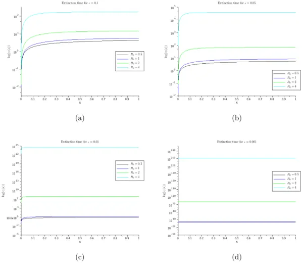
The asymptotic expression given by (28) confirms that, whenR0 >1, we can have a very long persistence of the disease before it is eventually extinct. Figure 10 displays the behaviour of τε(1/N) for different values of R0, with

N = 50, and confirms this first impression. Nevertheless, this result should be considered together with the results in Section 4; see the discussion in Section 7.

Figure 10: Mean extinction times for the disease when there is a single infected individual initially. Notice that even for such a moderate size pop-ulation, the mean time of extinction increases exponentially with R0. Simu-lations were performed with N = 50.

7. Conclusion

We have revisited the SIS model in two different classical formulations: the mass-action ODE model (SIS-ODE) and the discrete time Markov chain model (SIS-DTMC). As already observed by many authors (cf. Allen, 2008; N˚asell, 2011) the discrete version can have quite a different behaviour from the continuous one in many situations. This naturally leads to the search of a more comprehensive and unifying model.

Kampen, 2001), but following a more analytical route as pursued by the authors in Chalub and Souza (2009a,b) (and also more recently in Chalub and Souza (2013)) leads to a continuous equation for the probability density, that we term SIS-PDE, together with a boundary condition at one end, and with a conservation law.

Interestingly, this equation does not have classical solutions, but it admits measure solutions—which are unique. Such measure solutions are then the correct diffusion approximation of the system. This situation provides an example where the correct biological solution is not the most regular one.

This measure solution can be represented conveniently as

p(x, t) = a(t)δ0+r(x, t) (29) where r satisfies (13) and a is given by (14). The representation in (29) has a quite natural interpretation: r contains the probability of the transient states, and a the extinction probability. As is well-known, whenR0 >1 the SIS-DTMC model has a metastable state. Within the diffusion framework, the probability that governs such transient states (the quasi-stationary prob-ability) is associated to the principal eigenfunction of the classical version of the PDE.

The measure solution then contains, in a convenient representation, all the information about the model. This was also confirmed by several numerical examples, where we also can verify the good approximation properties of the diffusion model. In particular, we verify numerically that the ODE models the mode of the non-absorbed process if the initial infection is significant, or after some time is the initial infection is small.

These results then suggest that diffusion approximation, together with their correct mathematical set up can be useful as modelling tool. In par-ticular, they bring a powerful arsenal of analytical techniques that can con-tribute for the understanding of epidemiological problems, in the realm of finite population models.

Acknowledgments

FACCC: This work was partially supported by CMA/FCT/UNL, under the project PEst-OE/MAT/UI0297/2011. FACCC has also a “Investigador FCT” (FCT/Portugal) grant.

MOS: This work was partially supported by CNPq under the grant # 309616/2009-3 and by the PRONEX Dengue initiative, under CNPq grant # 550030/2010-7.

References

Allen, L. J., 1994. Some discrete-time SI, SIR, and SIS epidemic models. Mathematical Biosciences 124 (1), 83 – 105.

Allen, L. J. S., 2008. An introduction to stochastic epidemic models. In: Mathematical epidemiology. Vol. 1945 of Lecture Notes in Math. Springer, Berlin, pp. 81–130.

Allen, L. J. S., Burgin, A. M., 2000. Comparison of deterministic and stochas-tic SIS and SIR models in discrete time. Math. Biosci. 163 (1), 1–33. Anderson, R. M., May, R. M., 1995. Infectious diseases of humans: dynamics

and control, 1st Edition. Oxford science publications. Oxford University Press, Oxford, UK.

Bailey, N. T. J., 1963. The simple stochastic epidemic: A complete solution in terms of known functions. Biometrika 50 (3/4), pp. 235–240.

Bailey, N. T. J., 1975. The mathematical theory of infectious diseases and its applications, 2nd Edition. Hafner Press [Macmillan Publishing Co., Inc.] New York.

Cator, E., van de Bovenkamp, R., Van Mieghem, P., Jun 2013. Susceptible-infected-susceptible epidemics on networks with general infection and cure times. Phys. Rev. E 87, 062816.

Chalub, F. A. C. C., Souza, M. O., 2009a. From discrete to continuous evo-lution models: A unifying approach to drift-diffusion and replicator dy-namics. Theor. Popul. Biol. 76 (4), 268–277.

Chalub, F. A. C. C., Souza, M. O., 2009b. A non-standard evolution problem arising in population genetics. Commun. Math. Sci. 7 (2), 489–502. Chalub, F. A. C. C., Souza, M. O., 2011. The SIR epidemic model from a

PDE point of view. Math. Comput. Modelling 53 (7-8), 1568–1574. Chalub, F. A. C. C., Souza, M. O., 2013. The frequency-dependent

Wright-Fisher model: diffusive and non-diffusive approximations. J. Math. Biol.,

Forthcoming.

Diekmann, O., Heesterbeek, H., Britton, T., 2013. Mathematical tools for understanding infectious disease dynamics. Princeton, NJ: Princeton Uni-versity Press.

Dietz, K., 1975. Transmission and control of arbovirus diseases. In: Ludwig, D., Cooke, K. L. (Eds.), Epidemiology. SIAM, pp. 104–121.

Doering, C., Sargsyan, K., Sander, L., 2005. Extinction times for birth-death processes: Exact results, continuum asymptotics, and the failure of the fokker–planck approximation. Multiscale Modeling & Simulation 3 (2), 283–299.

Evans, L. C., 2010. Partial Differential Equations, 2nd Edition. Vol. 19 of Graduate Studies in Mathematics. American Mathematical Society, Prov-idence, RI.

Ewens, W. J., 2004. Mathematical population genetics, 2nd Edition. Vol. v. 27. Springer, New York.

Gardiner, C. W., et al., 1985. Handbook of stochastic methods. Springer Berlin.

Gillespie, D. T., 1976. A general method for numerically simulating the stochastic time evolution of coupled chemical reactions. Journal of Com-putational Physics 22 (4), 403 – 434.

Guo, H., Li, M. Y., Shuai, Z., 2006. Global stability of the endemic equi-librium of multigroup sir epidemic models. Can. Appl. Math. Q 14 (3), 259–284.

Hartfield, M., Alizon, S., 2013. Introducing the outbreak threshold in epi-demiology. PLoS Pathogens 9 (6), e1003277.

Hyman, J. M., Li, J., 1997. Behavior changes in sis std models with selective mixing. SIAM Journal on Applied Mathematics 57 (4), 1082–1094.

Keeling, M., Ross, J., 2008. On methods for studying stochastic disease dy-namics. Journal of The Royal Society Interface 5 (19), 171–181.

Lieberman, G., 1996. Second Order Parabolic Differential Equations. World Scientific.

Macdonald, G., 1957. The epidemiology and control of malaria. Oxford: Ox-ford University Press.

McKane, A. J., Newman, T. J., Oct 2004. Stochastic models in population biology and their deterministic analogs. Phys. Rev. E 70, 041902.

Mieghem, P. V., 2013. Non-markovian infection spread dramatically alters the susceptible-infected-susceptible epidemic threshold in networks. Phys-ical Review Letters 110 (10).

N˚asell, I., 2011. Extinction and Quasi-stationarity in the Stochastic Logistic SIS Model. Vol. 2022 of Lecture Notes in Math. Springer-Verlag.

Rass, L., Radcliffe, J., 2003. Spatial deterministic epidemics. Vol. 102 of Mathematical Surveys and Monographs. American Mathematical Society, Providence, RI.

Ross, R., 1911. The prevention of malaria., 2nd Edition. London: Murray. Taylor, M. E., 1996. Partial Differential Equations. I. Vol. 115 of Applied

Mathematical Sciences. Springer-Verlag, New York, basic theory. van Kampen, N., 2001. Stochastic processes in physics and chemistry. Van Segbroeck, S., Santos, F. C., Pacheco, J. M., 2010. Adaptive contact

net-works change effective disease infectiousness and dynamics. PLoS Comput Biol 6 (8).

Yang, G., 1972. Empirical study of a non-markovian epidemic model. Math-ematical Biosciences 14 (1–2), 65 – 84.