STATE-SPACE APPROACH TO EVALUATE THE RELATION BETWEEN SOIL PHYSICAL AND CHEMICAL PROPERTIES

(1)

STATE-SPACE APPROACH TO EVALUATE THE

RELATION BETWEEN SOIL PHYSICAL

AND CHEMICAL PROPERTIES

(1)

L. C. TIMM(2), K. REICHARDT(2), J. C. M. OLIVEIRA(3), F. A. M. CASSARO(4), T. T. TOMINAGA(2), O. O. S. BACCHI(2),

D. DOURADO-NETO(5) & D. R.NIELSEN(6)

SUMMARY

The state-space approach is used to evaluate the relation between soil physical and chemical properties in an area cultivated with sugarcane. The experiment was carried out on a Rhodic Kandiudalf in Piracicaba, State of São Paulo, Brazil. Sugarcane was planted on an area of 0.21 ha i.e., in 15 rows 100 m long, spaced 1.4 m. Soil water content, soil organic matter, clay content and aggregate stability were sampled along a transect of 84 points, meter by meter. The state-space approach is used to evaluate how the soil water content is affected by itself and by soil organic matter, clay content, and aggregate stability of neighboring locations, in different combinations, aiming to contribute to a better understanding of the relation among these variables in the soil. Results show that soil water contents were successfully estimated by this approach. Best performances were found when the estimate of soil water content at locations i was related to soil water content, clay content and aggregate stability at locations i-1. Results also indicate that this state-space model using all series describes the soil water content better than any equivalent multiple regression equation.

Index terms: spatial variability, sugarcane crop, kalman filter, auto-regressive model.

(1)_{Research funded by FAPESP, CAPES and CNPq. Recebido para publicação em agosto de 2002 e aprovado em novembro de} 2003.

(2)_{Researchers Soil Physics Laboratory, Centro Nacional de Energia na Agricultura, Universidade de São Paulo – CENA/USP.} Caixa Postal 96, CEP 13400-970 Piracicaba (SP).

(3) _{Professor Municipal University of Piracicaba – EEP. Caixa Postal 226, CEP 13414-040 Piracicaba (SP).}

(4)_{Professor Department of Physics, Universidade Estadual de Ponta Grossa – UEPG. Uvaranas, CEP 84051-510 Ponta Grossa} (PR).

(5)_{Professor Reteired Crop Production Department, Escola Superior de Agricultura “Luiz de Queiros” – ESALQ/USP. Caixa} Postal 9, CEP 13418-900 Piracicaba (SP).

(2)

RESUMO: ABORDAGEM DE ESPAÇO DE ESTADOS PARA AVALIAR A RELAÇÃO ENTRE PROPRIEDADES QUÍMICAS E FÍSICAS DO SOLO

A abordagem de espaço de estados é usada para avaliar a relação entre propriedades físicas e químicas de um solo em uma área cultivada com cana-de-açúcar. O experimento foi realizado em um Nitossolo situado em Piracicaba (SP). A cana-de-açúcar foi plantada em uma área de 0,21 ha i.e., 15 linhas com 100 m de comprimento cada, espaçadas de 1,4 m. Medidas da umidade do solo, matéria orgânica, conteúdo de argila e estabilidade de agregados foram feitas ao longo de uma transeção de 84 pontos, metro a metro. A abordagem de espaço de estados é usada para avaliar como a umidade do solo na posição i é afetada por medidas de umidade do solo, matéria orgânica, conteúdo de argila e estabilidade de agregados na posição i-1, em diferentes combinações, com o objetivo de contribuir para um melhor entendimento da relação entre estas variáveis no solo. Os resultados mostram que a umidade do solo pode ser estimada usando esta abordagem, sendo a melhor performance encontrada quando as estimativas da umidade do solo na posição i foram relacionadas com a umidade do solo, conteúdo de argila e estabilidade de agregados na posição i-1 e que as equações de espaço de estado descrevem a umidade do solo melhor do que qualquer equação de regressão múltipla equivalente.

Termos de indexação: variabilidade espacial, cana-de-açúcar, filtro de Kalman, modelo auto-regressivo.

INTRODUCTION

During the last decade, technologies to study specific local field conditions have rapidly developed, and can potentially help farmers manage each part of their farms with spatially varying intensities according to localized requirements or deficiencies. Relations among various soil, plant, and atmosphere variables across a field can be characterized with a quantitative accounting of errors involving measurements and models through the use of state-space analysis. The currently intuitive decision-making of farmers resembles the concepts of state-space analysis. They focus on crop responses associated with variations of local conditions prevailing at different locations within and among each of their fields (Nielsen et al., 1998). A linear system can be seen as a space representation of different states through two equations: one an observation vector and the other an evolution of the states. Predictions and estimates are obtained when the Kalman filter is applied to the model, representing states distributed in space (West & Harrison, 1997; Motta & Hotta, 1998). Classical statistics ignore sampling locations, and hence disregard the potential spatial dependence of observations within a field. In contrast, these newly applied methods in the field of soil science take advantage of spatial dependence by making use of the characteristics of each observation location. Statistical tools like autocorrelation function, semivariograms, and state-space, have been used recently to define the structure of spatial distributions of soil properties (Wendroth et al., 1992;

Katul et al., 1993; Wendroth et al., 1997; Hui et al., 1998; Dourado-Neto et al., 1999; Timm et al., 2000, 2003a,b). According to Bresler et al. (1981), research during the last two decades has focused the study of soil spatial variability on an improved understanding of processes that influence crop production variability. Nielsen & Alemi (1989) comment that in several reports using classical statistics, observations within and among treatments are not always independent, making the applied statistical design inadequate.

In this report, we present a state-space analysis of four sets of soil water content, soil organic matter, clay content, and aggregate stability, each observation made in a sugarcane field, under different management treatments, for a better understanding of the relation between these soil variables.

Theoretical aspects

In the state-space analysis, the state of a system of a variable, or of a set of variables measured at locations i, is related to the state of the same and other variables at locations i-h, where h( = 1,2,3,..., n) is the number of lags between neighbor observations. This autoregressive model is used for several types of predictions (and forecasts) based on space or time series, to identify coefficients that join these state systems (Wendroth et al., 1997).

A basic equation, called state equation, can be written for h = 1 as:

(3)

where Xi is the state vector (of a set of p variables) at location i; φ is a p x p matrix of state coefficients which indicates the measure of the regression; and

wi are noises of the system for i = 1,2,3,..., n. These values of noise are assumed to have zero mean, not to be correlated and to be normally distributed. This is the usual structure of a common autoregressive model, in which the coefficients of the matrix φ could be calculated by multiple regression, taking Xi and Xi-1 as the dependent and independent variables, respectively.

In the case of the state-space model, however, the true state of the variable is considered “embedded” in an observation equation:

Yi = Ai Xi + vi (2)

where the observation vector Yi is related to the state vector Xi by an observation matrix Ai (unit matrix, p x p) and an observation noise vector v_i, also considered of zero mean, not correlated and normally distributed. Inasmuch as the noises w_i and v_i are assumed to be independent of each other, the measurements need not be considered true, but can be seen as indirect measurements reflecting the true state of the variable added to a noise (Wendroth et al., 1997).

The state coefficients φpp and noises of equation (1) are estimated through a recursive procedure given by Shumway & Stoffer (1982). They are optimized by the Kalman filter (Kalman, 1960; Gelb, 1974) with an iterative algorithm. This filter is used to find optimized estimators for the state vector at positions i. Because the actual value of the state vector is sought or indeed required, Motta & Hotta (1998) state that this filter is frequently used in engineering, since it permits the estimation of the state vector with an ongoing renewal as new observations are obtained.

MATERIAL AND METHODS

Soil water content (SWC), soil organic matter (OM), clay content (CC), and aggregate stability (AS) were measured in a sugarcane experiment (Oliveira et al., 2001) in Piracicaba (SP), Brazil (22 o_{42 ´ S} and 47 o_{38 ´ W) on a Rhodic Kandiudalf, using a 84} point transect.

Soil water contents using a single gamma-neutron surface probe (model CPN, MC-3) were measured on September 6, 1999. With this probe water contents are measured by neutron moderation within a semi-sphere of about 0.15 m radius, observations representing the average SWC of the 0-0.15 m soil layer. Details of the calibration of this instrument can be found in Cassaro et al. (2000).

To determine the soil organic matter, clay content and aggregate stability, soil samples were collected

in a 0-0.15 m soil layer, along the 84 point transect. Soil organic matter was determined according to the methodology described by EMBRAPA (1997). The average value of soil organic matter was calculated from three soil organic matter data sets, which were measured at the beginning of the experiment (September 1997), after plant cane harvest (October 1998), and after the first ratoon cane harvest (October 1999). Clay content and aggregate stability were measured during the year 2000 (November 16, 2000). Details about these methods can be found in Gee & Bauder (1986) and Kemper & Rosenau (1986), respectively.

Data were analyzed by the state-space approach, using the software ASTSA (Applied Statistical Time Series Analysis) developed by Shumway (1988), under application of the transformation:

(

)

[

]

4s s 2 -m -X

xi= i (3)

where m is the mean of Xi and s the standard deviation. This transformation allows the state coefficients φpp in equation (1) to have magnitudes directly proportional to their contribution to each state variable used in the analysis (Hui et al., 1998). Note that transformed values xi of any variable have a mean of 0.5.

RESULTS AND DISCUSSION

(4)

Under these on-farm conditions, in the presence of heterogeneity, the effects of the different treatments on any of the measured variables are not easily ascertained by classical statistics, which ignore local spatial correlations. Under such conditions, according to Wendroth et al. (1998), local trends are best verified with nearest neighbor analysis.

other three sets of observations, aggregate stability has no discernible trend, and manifests spatial dependence up to only 3 lags.

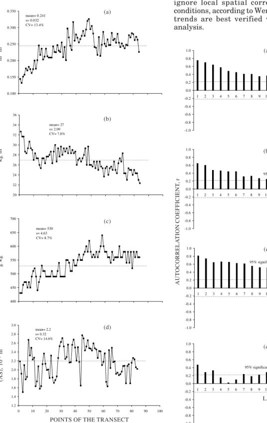
Figure 1. Soil water content on September 06, 1999 (a); soil organic matter (b); clay content (c); and aggregate stability distribution, meter by meter, along the 84 point transect (d).

POINTS OF THE TRANSECT

0.100 0.150 0.200 0.250 0.300 0.350 mean= 0.241 s= 0.032 CV= 13.4% A 20 22 24 26 28 30 32 34 36 mean= 27 s= 2.09 CV= 7.8% B 400 450 500 550 600 650 700 mean= 530 s= 4.63 CV= 8.7% C 1.2 1.4 1.6 1.8 2.0 2.2 2.4 2.6 2.8 3.0

0 10 20 30 40 50 60 70 80 90 100 mean= 2.2 s= 0.32 CV= 14.6% D SOIL W A

TER CONTENT (SWC),

m

3 m

-3

SOIL ORGANIC MA

TTER (OM), kg m -3 AGGREGA TE ST ABILITY (AS), 10

-3 m

CLA

Y CONTENT (CC),

g kg -1 (a) (b) (c) (d)

Figure 2. Calculated autocorrelation function (ACF) for soil water content data (a); soil organic matter data (b); clay content data of (1c) (c); and aggregate stability data (d).

AUT

OCORRELA

TION COEFFICIENT

, r

95% significance is 0.214 by "t" test

-1.0 -0.8 -0.6 -0.4 -0.2 0.0 0.2 0.4 0.6 0.8 1.0

1 2 3 4 5 6 7 8 9 10 11 12 13 14 15 16 17 18 19 20 Lags

-1.0 -0.8 -0.6 -0.4 -0.2 0.0 0.2 0.4 0.6 0.8 1.0

1 2 3 4 5 6 7 8 9 10 11 12 13 14 15 16 17 18 19 20 Lags

-1.0 -0.8 -0.6 -0.4 -0.2 0.0 0.2 0.4 0.6 0.8 1.0

1 2 3 4 5 6 7 8 9 10 11 12 13 14 15 16 17 18 19 20 Lags

A

-1.0 -0.8 -0.6 -0.4 -0.2 0.0 0.2 0.4 0.6 0.8 1.0

(5)

Traditionally, most agronomic investigations have used random (no correlation structure) sampling techniques and assumed independence between samples. Classical statistical analyses, such as ANOVA or regression analyses, are then performed to describe the changes observed within and among differently treated plots. Here we perform such analyses determining how well the set of soil water contents measured across the transect is described by classical regression equations.

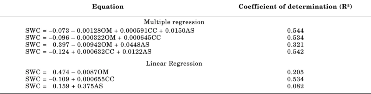
Because of the obvious spatial trends in at least three of the four sets of observations, we would expect that the variables would be related to each other. But ignoring the locations of the observations, we find that no more than 55 % of the variance of the soil water content data is explained by classical linear and multiple regression analyses using any combination among the observation sets. In table 1 we note that the best regression results are obtained using OM, CC, and AS, and the poorest by only AS. The use of CC and AS yields a multiple regression coefficient of determination nearly identical to the one obtained when using the three dependent variables.

These classical regression analyses are based on the assumption that each data set manifests, respectively, a constant mean along the entire transect, and ignores their local spatial crosscorrelations within the transect. The AS observations manifest only local spatial autocorrelation and do not have a trend to match those of the other observation sets, which accounts for the poor regression with soil water content.

We then verified if the use of applied time series analyses leads to additional information on the spatial variability of soil properties and, together with the classical statistical analyses (mean, standard deviation, and coefficient of variation), provides better management of the land, keeping soil losses at a minimum and helping to use natural resources more wisely.

The crosscorrelograms given in figure 3ab present a stronger spatial dependence between soil water content, soil organic matter, and clay content, respectively, than those presented in figure 3c between soil water content and aggregate stability. With such magnitudes of the crosscorrelation

functions, we recognize the potential for describing their distributions across the transect of observations with state-space analysis. Initially, in the context of the trends noted above, we are interested in an evaluation of how well the applied time series

-1.0 -0.8 -0.6 -0.4 -0.2 0.0 0.2 0.4 0.6 0.8 1.0

-10 -9 -8 -7 -6 -5 -4 -3 -2 -1 0 1 2 3 4 5 6 7 8 9 10

A

95% significance is 0.214by "t" test

-1.0 -0.8 -0.6 -0.4 -0.2 0.0 0.2 0.4 0.6 0.8 1.0

-10 -9 -8 -7 -6 -5 -4 -3 -2 -1 0 1 2 3 4 5 6 7 8 9 10

B

-1.0 -0.8 -0.6 -0.4 -0.2 0.0 0.2 0.4 0.6 0.8 1.0

-10 -9 -8 -7 -6 -5 -4 -3 -2 -1 0 1 2 3 4 5 6 7 8 9 10

C

Figure 3. Calculated crosscorrelogram function (CCF) between soil water content and soil organic matter data (a); soil water content and clay content data (b); and soil water content and aggregate stability data (c).

CROSS CORRELA

TION COEFFICIENT

,

rc

LAGS

(a)

(b)

(c)

Equation Coefficient of determination (R2₎

Multiple regression

SWC = –0.073 – 0.00128OM + 0.000591CC + 0.0150AS 0.544

SWC = –0.096 – 0.000322OM + 0.000645CC 0.534

SWC = 0.397 – 0.00942OM + 0.0448AS 0.321

SWC = –0.124 + 0.000632CC + 0.0122AS 0.542

Linear Regression

SWC = 0.474 – 0.0087OM 0.205

SWC = –0.109 + 0.000655CC 0.534

SWC = 0.159 + 0.375AS 0.082

(6)

analysis can describe the soil water content series using various combinations of the soil organic matter, clay content, and aggregate stability series. Each series has been transformed to the same mean through equation (3).

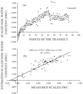
Figure 4a presents the state-space analysis applied to soil water content, soil organic matter, clay content, and aggregate stability with the open circle symbol representing the measured soil water content. The middle line represents the predicted values of soil water content using the state equation. The upper and the lower lines represent the fiducial limits which take a plus or minus two standard deviation, respectively, into consideration. It can be seen from the equation in the figure that the soil water content at location i-1 contributes with about 91 % to the estimate of the soil water content in location i, while organic matter, clay content, and aggregate stability at location i-1 contribute 7, 6, and 2.4 %, respectively. Figure 4b indicates that this state-space model under use of all four series describes the soil water content (R2_{= 0.797) better than the} equivalent multiple regression equation (R2_{= 0.544).} Figure 5 presents the state-space analysis of soil water content ignoring the aggregate stability series. Here, in comparison to the graphs in figure 4, the contribution from soil water content at location i-1

is somewhat lower, the fiducial limits are wider, and R2_{is greater (0.836).}

Data in table 2 show that the state-space equations describe the soil water content better than any of the respective classical regression equations (Table 1).

Among the results given in table 2, we identified the best performance of all the state-space equations as the one using clay content and aggregate stability. For this equation, the contribution of soil water contents from location i-1 was the smallest and R2 the greatest. In other words, the local and regional variations of CC and AS across the transect were the most important variations in relation to the spatial distribution of SWC.

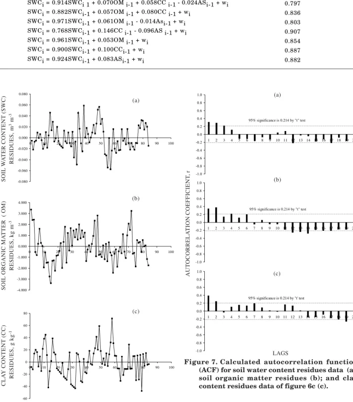
Next, we removed the spatial trends (shown in Figure 1abc) using a second order polynomial regression equation for each of the three sets of observations. Subtracting these trends from each of their respective sets of observations yielded the residues plotted along the transect in figure 6abc. The autocorrelation functions of these residues shown in figure 7abc reveal that a spatial dependence across at least 2 lags persisted after the detrending process. In other words, values of each of the observations were still related to those of their

Figure 5. State-space analysis of scaled soil water content data as a function of scaled soil water content, scaled soil organic matter and scaled clay content at location i-1 (a); correlation between estimated and measured scaled soil water content data of (a) (b).

(SWC) est = 0.7585 * (SWC) mea + 0.1220 R2_{= 0.8359}

-0.400 -0.200 0.000 0.200 0.400 0.600 0.800 1.000

-0.400 -0.200 0.000 0.200 0.400 0.600 0.800 1.000 1.200

Measured scaled SWC

E sti ma te d sc al e d S W C B

SCALED SOIL W

A

TER

CONTENT (SWC)

MEASURED SCALED SWC (SWC)i = 0.8816 * (SWC)i-1 + 0.0572 * (OM)i-1 + 0.0798 * (CC)i-1 + w(swc)i

-0.400 -0.200 0.000 0.200 0.400 0.600 0.800 1.000 1.200

0 10 20 30 40 50 60 70 80 90 100

Points of the transect

measured

POINTS OF THE TRANSECT (a)

(b)

ESTIMA

TED SCALED SOIL

W

A

TER

CONTENT (SWC)

Figure 4. State-space analysis of scaled soil water content data as a function of scaled soil water content, scaled soil organic matter, scaled clay content and scaled aggregate stability at location i-1 (a); correlation between estimated and measured scaled soil water content data of (a) (b).

SCALED SOIL W

A

TER

CONTENT (SWC)

(SWC)i = 0.9141 * (SWC)i-1 + 0.0702 * (OM)i-1 + 0.0584 * (CC)i-1 - 0.0235 * (AS)i-1 + w(swc)i -0.400 -0.200 0.000 0.200 0.400 0.600 0.800 1.000 1.200

0 10 20 30 40 50 60 70 80 90 100

Points of the transect

measured

(SWC) est = 0.7781 * (SWC) mea + 0.1108 R2_{= 0.7972}

-0.400 -0.200 0.000 0.200 0.400 0.600 0.800 1.000

-0.200 0.000 0.200 0.400 0.600 0.800 1.000 1.200 Measured scaled SWC

Es ti m at ed s cale d S W C B

MEASURED SCALED SWC (a)

(b)

ESTIMA

TED SCALED SOIL W

A

TER

(7)

respective neighboring values. Further analysis revealed that three of the four series were spatially crosscorrelated – aggregate stability, clay content and organic matter. Although soil water content Figure 6. Soil water content residues distribution

(a); soil organic matter residues distribution, (b); and clay content residues distribution, meter by meter, along the 84 point transect (c).

SOIL W

A

TER CONTENT (SWC)

RESIDUES, m

3 m

-3

(b)

(c)

SOIL ORGANIC MA

TTER ( OM)

RESIDUES, kg m

-3

CLA

Y CONTENT (CC)

RESIDUES, g kg

-1

-0.080 -0.060 -0.040 -0.020 0.000 0.020 0.040 0.060 0.080

0 10 20 30 40 50 60 70 80 90 100

A

-4.000 -3.000 -2.000 -1.000 0.000 1.000 2.000 3.000 4.000

0 10 20 30 40 50 60 70 80 90 100

B

-60 -40 -20 0 20 40 60 80

0 10 20 30 40 50 60 70 80 90 100

Points of the transect C

(a)

(c)

Figure 7. Calculated autocorrelation function (ACF) for soil water content residues data (a); soil organic matter residues (b); and clay content residues data of figure 6c (c).

AUT

OCORRELA

TION COEFFICIENT

, r

-1.0 -0.8 -0.6 -0.4 -0.2 0.0 0.2 0.4 0.6 0.8 1.0

1 2 3 4 5 6 7 8 9 10 11 12 13 14 15 16 17 18 19 20 Lags

A

-1.0 -0.8 -0.6 -0.4 -0.2 0.0 0.2 0.4 0.6 0.8 1.0

1 2 3 4 5 6 7 8 9 10 11 12 13 14 15 16 17 18 19 20 Lags

B

95% significance is 0.214 by "t' test

-1.0 -0.8 -0.6 -0.4 -0.2 0.0 0.2 0.4 0.6 0.8 1.0

1 2 3 4 5 6 7 8 9 10 11 12 13 14 15 16 17 18 19 20 Lags

C

LAGS (a)

(b)

(c)

Equation Coefficient of determination (R2₎

SWCi = 0.914SWCi 1 + 0.070OM i-1 + 0.058CC i-1 - 0.024ASi-1 + wi 0.797

SWCi = 0.882SWCi-1 + 0.057OM i-1 + 0.080CC i-1 + wi 0.836

SWCi = 0.971SWCi-1 + 0.061OM i-1 - 0.014Asi-1 + wi 0.803

SWCi = 0.768SWCi-1 + 0.146CC i-1 - 0.096AS i-1 + wi 0.907

SWCi = 0.961SWCi-1 + 0.053OM i-1 + wi 0.854

SWCi = 0.900SWCi-1 + 0.100CCi-1 + wi 0.887

SWCi = 0.924SWCi-1 + 0.083ASi-1 + wi 0.882

Table 2. State-space equations of soil water content (SWC) using the soil organic matter data (OM), clay

content data (CC), aggregate stability data (AS), and values of R2 from linear regression between

(8)

was autocorrelated, it was not crosscorrelated with any of the other variables. Hence, its spatial variation cannot be related to the spatial variability of AS, CC, and OM.

Proceeding without the SWC series, we used the state-space analysis to describe the aggregate stability series in terms of clay content and organic matter (Figure 8 and Table 3). Using both series of

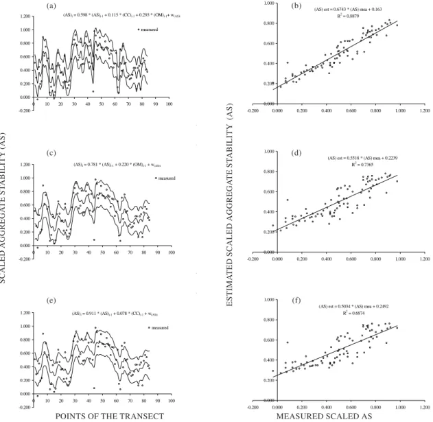
Figure 8. State-space analysis of scaled original aggregate stability data: as a function of scaled original aggregate stability, scaled clay content residues and scaled soil organic matter residues, all at location i-1 (a); correlation between estimated and measured scaled original aggregate stability data of (a) (b); as a function of scaled original aggregate stability and scaled soil organic matter residues, all at location i-1 (c); correlation between estimated and measured scaled original aggregate stability data of (c) (d); as a function of scaled original aggregate stability and scaled clay content residues, all at location i-1 (e); and correlation between estimated and measured scaled original aggregate stability data of (e) (f).

POINTS OF THE TRANSECT MEASURED SCALED AS

SCALED AGGREGA

TE ST

ABILITY (AS)

(AS)i = 0.598 * (AS)i-1 + 0.115 * (CC)i-1 + 0.293 * (OM)i-1+ w(AS)i

-0.200 0.000 0.200 0.400 0.600 0.800 1.000 1.200

0 10 20 30 40 50 60 70 80 90 100 Points of the transect

measured

A (AS) est = 0.6743 * (AS) mea + 0.163

R2

= 0.8879

0.000 0.200 0.400 0.600 0.800 1.000

-0.200 0.000 0.200 0.400 0.600 0.800 1.000 1.200 Measured scaled AS

Estimated scaled AS

B

(AS)i = 0.781 * (AS)i-1 + 0.220 * (OM)i-1 + w(AS)i

-0.200 0.000 0.200 0.400 0.600 0.800 1.000 1.200

measured

C (AS) est = 0.5518 * (AS) mea + 0.2239

R2

= 0.7365

0.000 0.200 0.400 0.600 0.800 1.000

-0.200 0.000 0.200 0.400 0.600 0.800 1.000 1.200 Measured scaled AS

Estimated scaled AS

D

(AS)i = 0.911 * (AS)i-1 + 0.078 * (CC)i-1 + w(AS)i

-0.200 0.000 0.200 0.400 0.600 0.800 1.000 1.200

measured

E (AS) est = 0.5034 * (AS) mea + 0.2492

R2

= 0.6874

0.000 0.200 0.400 0.600 0.800 1.000

-0.200 0.000 0.200 0.400 0.600 0.800 1.000 1.200

Estimated scaled AS

F (a)

(c)

(e)

(b)

(d)

(f)

ESTIMA

TED SCALED AGGREGA

TE ST

ABILITY (AS)

Table 3. State-space equations of aggregate stability using the soil organic matter residues data, clay

content residues data, and values of R2_{from linear regression between estimated and measured}

values of AS. All observations have been scaled using equation (3)

Equation Coefficient of determination R2

ASi = 0.598ASi-1 + 0.115CCi-1 + 0.293OMi-1 + w i 0.888

ASi = 0.781ASi-1 + 0.220OMi-1 + w i 0.736

(9)

OM and CC yields the best description of aggregate stability - the contribution of aggregate stability from location i-1 was the smallest, and R2_{was the} greatest. Moreover, we note that using OM rather than CC in combination with AS yields a better description of AS.

The results given in tables 1, 2 and 3 reveal that spatial variations of OM and CC are significantly related to variations of SWC and AS across the measured transect. Because these state-space equations are empirical, we only know that the spatial variations of the various sets of observations are related to each other, but we still have to identify why they are related. In the future we shall learn that physical or chemical laws can be incorporated into state-space equations allowing for a more judicious selection of adequate variables as input information, and providing a more realistic explanation of the local and regional spatial and temporal processes occurring in a farmer’s field and across the landscape. It is shown that the state-space analysis under field conditions is able to account for the underlying processes between several variables in each and every local neighborhood within a field. Using this analysis, it is possible to identify a variable that relates to the local behavior of several other variables and stochastically quantify that relationship accounting for both measurement and model errors. The analysis presented here relates soil properties at sites i to neighbors at sites i-1 and is a powerful tool for precision agriculture, of potential importance to farmers since it opens the possibility to examine physical and chemical properties that affect the crop yield within heterogeneous fields. Such an examination gives them specific ideas about how to better farm management, and consequently increase crop production and simultaneously improve the quality of the local environment.

LITERATURE CITED

BRESLER, E.; DASBERG, S.; RUSSO, D. & DAGAN, G. Spatial variability of crop yield as a stochastic soil process. Soil Sci. Soc. Am. J., 45:600-605, 1981.

CÁSSARO, F.A.M.; TOMINAGA, T.T.; BACCHI, O.O.S.; REICHARDT, K.; OLIVEIRA, J.C.M. & TIMM, L.C. Improved laboratory calibration of a single probe surface gamma neutron gauge. Austr. J. Soil Res., 38:937-946, 2000. DOURADO-NETO, D.; TIMM, L.C.; OLIVEIRA, J.C.M.; REICHARDT, K.; BACCHI, O.O.S.; TOMINAGA, T.T. & CASSARO, F.A.M. State-space approach for the analysis of soil water content and temperature in a sugarcane crop. Sci. Agric., 56:1215-1221, 1999.

EMPRESA BRASILEIRA DE PESQUISA AGROPECUÁRIA -EMBRAPA. Centro Nacional de Pesquisas de Solos. Manual de métodos de análise de solo. 2.ed. Rio de Janeiro, 1997. 212p.

GEE, G.W. & BAUDER, J.W. Particle-size analysis. In: KLUTE, A., ed. Methods of soil analysis. 2.ed. Madison, American Society of Agronomy and Soil Science Society of America, 1986. p.383-423.

GELB, A. Applied optimal estimation. Cambridge, Massachusetts Institute of Technology Press, 1974. 374p. HUI, S.; WENDROTH, O.; PARLANGE, M.B. & NIELSEN, D.R. Soil variability – Infiltration relationships of agroecosystems. J. Balkan Ecol., 1:21-40, 1998.

KALMAN, R.E. A new approach to linear filtering and prediction theory. Trans, ASME, J. Basic Eng., 8:35-45, 1960. KATUL, G.G.; WENDROTH, O.; PARLANGE, M.B.; PUENTE,

C.E.; FOLEGATTI, M.V. & NIELSEN, D.R. Estimation of in situ hydraulic conductivity function from nonlinear filtering theory. Water Res. Res., 29:1063-1070, 1993. KEMPER, W.D. & ROSENAU, R.C. Aggregate stability and

size distribution. In: KLUTE, A., ed. Methods of soil analysis. 2.ed. Madison, American Society of Agronomy and Soil Science Society of America, 1986. p.425-442. MOTTA, A.C.O. & HOTTA, L.K. Utilização do filtro de Kalman

em modelos estatísticos. Campinas, Instituto de Matemática, Estatística e Computação Científica, UNICAMP, 1998. 71p.

NIELSEN, D.R.; WENDROTH, O. & PIERCE, F.J. Emerging concepts for solving the enigma of precision farm research. In: INTERNATIONAL CONFERENCE ON PRECISION AGRICULTURE, 4., Saint. Paul, 1998. Proceedings. Saint. Paul, ASA-CSSA-SSSA, 1998. p.303-318.

NIELSEN, D.R. & ALEMI, M.H. Statistical opportunities for analyzing spatial and temporal heterogeneity of field soils. Plant Soil, 115:285-296, 1989.

OLIVEIRA, J.C.M.; TIMM, L.C.; TOMINAGA, T.T.; CASSARO, F.A.M.; REICHARDT, K.; BACCHI, O.O.S.; DOURADO-NETO, D. & CAMARA, G.M.S. Soil temperature in a sugar-cane crop as a function of the management system. Plant Soil, 230:63-68, 2001.

SHUMWAY, R.H. & STOFFER, D.S. An approach to time series smoothing and forecasting using the EM algorithm. J. Time Series Anal., 3:253-264, 1982.

SHUMWAY, R.H. Applied statistical time series analyses. New York, Prentice Hall, Englewood Cliffs, 1988. 379p. TIMM, L.C.; BARBOSA, E.P.; SOUZA, M.D.; DYNIA, J.F. &

REICHARDT, K. State-space analysis of soil data: an approach based on space-varying regression models. Sci. Agric., 60:371-376, 2003a.

TIMM, L.C.; REICHARDT, K.; OLIVEIRA, J.C.M.; CÁSSARO, F.A.M.; TOMINAGA, T.T.; BACCHI, O.O.S. & DOURADO-NETO, D. Sugarcane production evaluated by the state-space approach. J. Hydrol., 272:226-237, 2003b.

TIMM, L.C.; FANTE JUNIOR, L.; BARBOSA, E.P.; REICHARDT, K. & BACCHI, O.O.S. A study of the interaction soil – plant using state-space approach. Sci. Agric., 57:751-760, 2000.

(10)

WENDROTH, O.; REYNOLDS, W.D.; VIEIRA, S.R.; REICHARDT, K. & WIRTH, S. Statistical approaches to the analysis of soil quality data. In: GREGORICH, E.G. & CARTER, M.R., eds. Soil quality for crop production and ecosystem health. Amsterdam, Elsevier Science, 1997. p.247-276.

WENDROTH, O.; AL OMRAN, A.M.; KIRDA, K.; REICHARDT, K. & NIELSEN, D.R. State-space approach to spatial variability of crop yield. Soil Sci. Soc. Am. J., 56:801-807, 1992.