1 FEAGRI/UNICAM P, Cidade Universitária Zeferino Vaz S/N, C.P. 6011, CEP 13083-875, Campinas, SP. Fone: (19) 3521-1069; (19) 3521-1053. E-mail: [email protected]; [email protected]; [email protected]
2 FCAV/UNESP, CEP 14884-900, Jaboticabal, SP. Fone: (16) 3209-2601. E-mail: [email protected]
Spatial variability of soil attributes and sugarcane yield
in relation to topographic location
Zigomar M . de Souza1, D omingos G. P. Cerri1, Paulo S. G. M agalhães1 & D iego S. Siqueira2
ABSTRACT
Soils submitted to the same management system in places with little variation of landscape, manifest differentiated spatial variability of their attributes and crop yield. The aim of this work was to investigate the correlation betw een spatial variability of the soil attributes and sugarcane yield as a result of soil topography. To achieve this objective, a test area of 42 ha located at the São João Sugar Mill, in Araras, in the State of São Paulo, Brazil, w as selected. Sugarcane yield w as measured w ith a yield monitor fitted in a sugarcane harvester and GPS signal. A total of 170 soil samples w ere taken at regular 50 m grid, at a depth of 0 - 0.2 m. The area under study was divided into two sites based on topography. The following soil attributes w ere analysed: organic matter (OM) content, exchangeable potassium (K), calcium (Ca) and magnesium (M g), their base saturation percentage (%BS), cation exchange capacity (CEC), pH, clay, silt, total sand and density. The use of landscape and geostatistics enable defining areas with different spatial variability in soil attributes and crop yield, providing the visualization and definition of homogeneous management zones. The largest spatial variability of soil attributes and sugarcane yield w as in the lowest part of the field.
Key words: Saccharum sp, geostatistics, semivariogram, curvature, precision agriculture
Variabilidade espacial de atributos do solo
e produtividade da cultura de cana-de-açúcar
em relação a localização topográfica
RESU M O
Solos submetidos ao mesmo sistema de manejo em locais com pequena variação de relevo manifestam variabilidade espacial diferenciada de atributos do solo e das plantas. Objetivou-se com este trabal ho estudar a correl ação entre a variabilidade espacial de atributos físicos e químicos do solo com a produtividade da cana-de-açúcar em duas posições do relevo, de acordo com a topografia da área. O estudo foi realizado no município de Araras, SP, em uma área de 42 ha, pertencente à Usina São João. Para o mapeamento da produti vi dade da cul tura da cana-de-açúcar uti li zou-se um moni tor de produtividade acoplado à colhedora e ao sinal de GPS. Coletaram-se 170 amostras do solo, em uma malha regular de 50 m entre pontos, na profundidade de 0,0 - 0,2 m. O talhão de estudo foi dividido em duas áreas menores, segundo a topografia. O s atributos do solo avaliados foram: teor de matéria orgânica (M O), potássio (K), cálcio (Ca), magnésio (Mg), saturação por bases (V%), capacidade de troca catiônica (CTC), pH , argila, silte, areia total e densidade. O uso do relevo e da geoestatística possibilitou definir áreas com diferentes variabilidades espaciais para atributos do solo e produtividade da cultura de cana-de-açúcar, proporcionando a visualização e definição de zonas homogêneas de manejo de acordo com o relevo. A maior variabilidade espacial de atributos do solo e a produtividade da cultura de cana-de-açúcar ocorreram na parte mais baixa do talhão.
Palavras-chave: Saccharum sp, geoestatística, semivariograma, curvatura, agricultura de precisão Revista Brasileira de
Engenharia Agrícola e Ambiental
v.14, n.12, p.1250–1256, 2010
I
NTRODUCTIONSoil spatial variability appears since formation and continues after the soil reaches its dynamic balance. This fact occurs because the parent material is not uniform due to differences in relation to hardness, chemical composition, crystallization, exposition, location, and also from the differences in climate and biological organisms present in its composition. Factors, such as slope, topography and relief forms, influence the physical attributes of the soil such as permeability, porosity, particle size, horizon thickness, water infiltration rate and erosion and also the yield in an indirect way.
Kravchenko & Bullock (2000) studied the correlation of corn and soybean production with landscape position and soil chemical attributes, and verified that topography by itself was not as informative as soil attributes, but for some fields, soil attributes in combination with topography explained as much as 78% of the yield variability. Lower yields were observed at higher landscape positions, demonstrating a negative correlation with soil elevation.
The spatial variability of soil attributes in different landscape positions can be determined using geostatistics techniques. Studies have shown that concave and convex oxisol areas, notwithstanding past management, present more chemical and physical attributes variability than flat shaped areas (Souza et al., 2003; 2004).
The spatial variability of soil attributes is also influenced by water flow, which is related to the landscape, because the preferential water routes define the most important erosion-deposit mechanisms (Alba, 2003). Silva & Alexandre (2005) evaluating the spatial variability of spray irrigated corn yield in the presence of complex topography and soil attributes, concluded that topographical information can be especially helpful in site-specific management for delineating areas where crop yields are more sensitive to extreme water conditions.
Understanding how the spatial distribution of the physical and chemical soil attributes works is important to establish adequate management practices, not only in terms of agricultural production optimization but also to lessen possible environmental damage. Pennock (2003) demonstrated that field topographical variations can be observed through digital elevation models (DEM), and those variations lead to an understanding of the pattern and distribution of water flows in land, allowing establishing relationships between the shapes of the relief and the variability of the soil attributes. USDA-NRCS (2002) recommends that for soil collection and description in the field, the observation of the landscape curvature and profile using the geomorphologic models proposed by Troeh (1965) should be used. These profiles of curves have been aiding in understanding the space variability of soil attributes (Souza et al., 2004).
The main aim of the study reported in this paper was to evaluate topography, soil attributes and sugarcane yield relationship. The hypothesis was that it is possible to explain the sugarcane yield variability when soil attributes are related to topography.
M
ATERIAL ANDMETHODSThe study area
The research was carried out in a 42 ha sugarcane area at the sugarcane mill “Usina São João Açúcar e Álcool”, in Araras. The area is located 166 km north of São Paulo city, southeast Brazil, at 22o 23’ 20" S and 47o 27’ 04" W, with average altitude of 657 m. The climate in the region is the CWa, mesothermic, with dry winters according to the Köppen system. Rain fall pattern follows typical low altitude tropical zones, rainy summers and dry winters. The average rainfall was 1.690 mm in 2003-2004 season. Based on the research carried out in a 1:20.000, scale, the soils are predominantly Oxisol, specifically Typic Haplustox. The sugarcane variety planted in 2001 in the study area was SP80-1816, on its third harvest. The sugarcane in this area is mechanically green harvested.
Soil sampling
Soil samples were collected in the fall of 2003 using a regular grid of 50 x 50 m with a soil probe to a depth of 0.0 - 0.2 m. A total of 170 samples were taken and each sample was composited from three cores collected within a 5 m radius. The sample points were geo-referenced with a GPS receiver (GEOExplorer III, Trimble Navigation Limited) and corrected by post-process differential signal, using correction files obtained from the Escola Superior “Luiz de Queiroz” (ESALQ/USP) referential base station located 20 km to the southwest of the area.
Topography
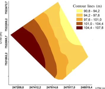
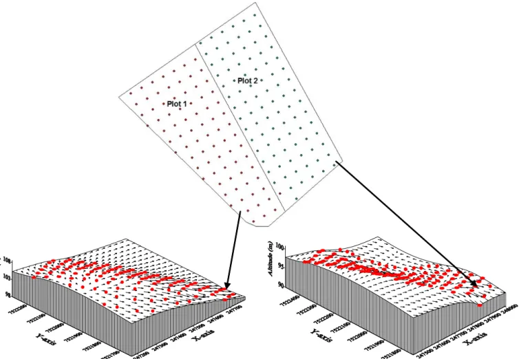
The slope of the area is not greater than 12%, value limits for mechanical harvesting, due to limitations of the sugarcane harvesters. After the topography survey the area was divided in two plots (Figure 1). In the higher elevation part of the area 80 samples were collected (Plot 1) and in the lower elevation part 90 samples were taken, predominantly with a concave curvature (Plot 2). Both areas had a maximum elevation difference of 10 m.
Figure 1. Topography survey of the study area
Troeh (1965) model presents nine basic types of landforms that are represented by letters C (curvature) and P (profile), both complemented by the signs (+) for concavity (form that favours the concentration of water), (-) for convexity (form that favours the dispersion of water) and (0) linearity. Figure 2 shows the soil profile of the area classified in accordance to this model. It is possible to observe in Plot 1 the predominance of linear form (C0P0) and in Plot 2 the concave form (C+P+). The program Surfer (Golden Software, 1999) was used to obtain the Digital Elevation Model (DEM) of the area, showing the forms of the relief and vectors representing the superficial path (arrows) and intensity (size of the arrow) of the water flow.
To carry out the digital analysis a map was generated based on the “Irregular Triangular Network” (ITN). The considered attributes were elevation, slope and curvature at each point of the surface. The slope represents the first derivative of the altitude and corresponds to the declivity of the soil surface in relation to the horizontal plan calculated directly from ITN. The curvature and profile of the soil surface represent the second derivative of the altitude, calculated from Troeh (1965) model.
The measured soil attributes were organic matter (OM) content, pH in CaCl2, available phosphorus (P), exchangeable potassium (K), calcium (Ca), and magnesium (Mg), extracted using the ion change resin method proposed by Raij et al. (2001). Cation exchange capacity (CEC) and their base
saturation percentage (%BS) were calculated based on the chemical analysis. The particle-size analysis was carried out using the hydrometric method (EMBRAPA, 1997). The soil density was determined by the volumetric cylinder method described by EMBRAPA (1997).
In agreement with the DEM and the Troeh (1965) model topographic variation of the landscape was observed (Figure 2). These models favor the understanding of the erosion processes and deposition of sediments and the redistribution of the soils along the landscape. From these models, it was possible to verify the pattern and distribution of the water flows in the soil surface to establish the relationships between the land forms and the variability of the soil attributes.
Yield mapping
To map sugarcane yield, a sugarcane harvester (Case 7700) equipped with a yield monitor designed by Magalhães & Cerri (2007) was used. The area to be mapped was divided into cells, which dimensions were function of: speed and harvesting width of the combine; data reading capacity; acquisition rate of the measurement; and positioning system. Considering a harvesting speed of 1.38 m s-1, sugarcane row spacing of 1.5 m, the fact that the combine only harvests one row at time and a period of 10 s for data acquisition, the average size of the cells adopted were 20 m2.
Figure 2. Di gital terrain model (DTM ) of the studied areas and the direction of water flow () and sample gri d (50 x 50 m) for the sampling of physical and chemical soil attri butes (red points)
The elimination of data acquisition errors is an important factor in obtaining a good quality result. Therefore, the data collected were processed to remove outliers and artefacts and to better align the yield spatially. Null and negative yield values were removed. Yield values in the top 0.5 and bottom 2.5 percentiles were disregarded in agreement with a methodology proposed by Tukey (1977). A three second delay was added to the yield data to account for the time lag that occurs between the time sugar cane is harvested and the time it reaches the yield sensor.
Correlation between the soil’s physical and chemical attributes with sugar cane yield
Because the yield maps were created using the data from 20 m2 cells and the soil maps were generated from a 50 x 50 m grid, yield values were averaged within a 20 m radius from the soil sample location (Molin et al., 2001) using ArcGis software to correlate the sugarcane yield with soil attributes.
For all statistical correlation and regression analysis, the average for each of the physicochemical attributes analysed over the root zone layer (0.0 - 0.20 m) at each collection point was used. Yield responses to individual soil attributes were modelled using a correlation index (5% significance) using Statgraph Plus for Windows 4.1.
Statistical analyses
After data filtering, ArcGis 8.3 software was used to create the sugarcane yield map and the physical and chemical soil attributes maps. All geostatistical analyses were performed using the Geostatistical Analyst extension of this software. The kriging was used as an interpolation method for sugarcane yield and soil samples.
The soil variability was evaluated by exploratory data analysis, first testing the normality, then calculating the mean, standard deviation, median, coefficient of variation (CV), asymmetry and the kurtosis coefficient; and the maximum and minimum values. The spatial variation was calculated by the semivariogram method (Journel & Huijbregts, 1991) using the regionalized variable theory, which assumes the stationary and the intrinsic hypothesis.
The semivariance was estimated by the Eq. 1:
) h ( N 1 i 2 i i) Z(x h)x ( Z ) h ( N 2 1 ) h ( ˆ where:
N(h) is number of paired measured points Z(xi), Z(xi + h), separated by a vector h. The graph plotted from ˆ(h) and the corresponding h value is called a semivariogram.
The coefficients of the theoretical semivariogram model (nugget effect, C0; sill, C0 + C1; range) were determined by the fitness of the mathematical model. The following models were fitted to the data: (a) spherical (Sph) Eq. 2 e (b) exponential (Exp) Eq. 3.
a h for C C a h 0 for a h 5 . 0 a h 5 . 1 C C ) h ( ˆ 1 0 3 1 0
for 0 h
a h exp 1 C C ) h (
ˆ 0 1
The semivariogram examination by the GS+ software (Gamma Design Inc., Plainwell, MI) was used for spatial dependence determination. When more than one variogram could be used, the most appropriate was chosen by the cross-validation (“jack-knifing”) method. To analyze the level of spatial dependence of the attributes under study, the classification proposed by Cambardella et al. (1994) was used, where the semivariograms are considered to be strongly spatially dependent when the nugget effect is less than or equal to 25% of the sill, moderate when between 25 to 75% and weak when greater than75%.
The correlation coefficients between sugarcane yield and soil chemical and physical attributes were calculated to explain the crop yield as a function of topography and water flow (95% confidence level).
R
ESULTSANDDISCUSSIONStatistical data analysis
The descriptive data analysis for the two areas is presented in Table 1. It is possible to observe large amplitude of the soil chemical attributes. These results are in agreement with those obtained by Corá et al. (2004) and Souza et al. (2004), who studied the spatial variability of the soil chemical attributes in sugarcane crop. The large amplitude reveals the problems that can occur when the average values for fertility management are used.
The results of the Kolmogorov-Smirnov test (Table 1) indicated normality for soil density, CEC, %BS and pH. According to Isaaks & Srivastava (1989) more important than the normality of the data is that the values of the mean and medians should not be far-off and that the asymmetry coefficients and kurtosis should be close to zero. Only Ca, Mg and CEC presented values of kurtosis great than 2.2 in both plots.
The Coefficients of Variation (CV) are dimensionless and allow the comparison of values between different soil attributes. High CV values could be considered the first indication of data heterogeneity (Frogbrook et al., 2002). The variability of a soil attribute can be classified by Warrick & Nielsen (1980) based on CV (Table 1). The variability of clay, silt, total sand, soil density, OM, pH, CEC, %BS and yield was low (CV < 30%) in both plots. However, the Ca, Mg and K attributes presented a high CV (CV > 30%) in both plots. Among the attributes analyzed, it was observed that greater values of CV occurred in the region with the lowest elevation of the area (Plot 2) indicating a greater variability in this area in relation to the (1)
(2)
region with highest elevation of the area (Plot 1), probably due to the presence of an expressive concavity in the area differentiating water flow.
The results of the geostatistics analysis show that all the variables analyzed presented spatial dependence (Table 2). The spherical model fitted itself to the data of all the studied variables, with the exception of the silt and K in Plot 2 and the pH in Plot 1, which fitted to the exponential model. Mcbratney & Webster (1986) studied semivariogram adjustment models for soil attributes and reported that the spherical and exponential models are those most frequently found.
The analysis of the relative nugget effect C0/(C0 + C1) showed a strong level of spatial dependence for all the studied variables, with the exception of silt, OM and pH in Plot 1 and K and OM in Plot 2, which present a moderate level of spatial dependence (Table 2). This demonstrates that the semivariograms explain the greater part of the experimental data variance.
The soil granulometric attributes, OM and sugarcane yield present the highest semivariogram directional range in the two areas, and the chemical attributes present the lowest values (Table 2). The lower the range, the faster independence is reached between samples, as the directional range is the distance limit of spatial dependence. Then extrinsic variability, relative to soil management practices, contributes towards range reduction.
Correlation
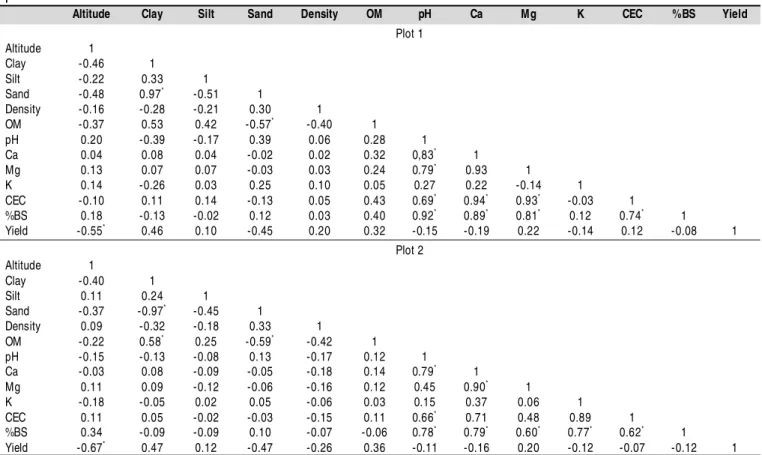
It is observed in Table 3 that the attributes altitude, clay, sand and OM presented the highest correlations with sugarcane yield in the areas with concaves and linear landform. The
Table 1. Descriptive statistics for the physical and chemical attributes in different topographic positions
1 Standard deviation
2 d = Statistics from the Kolmogorov-Smirnov test
ns non- significant 5% probability
Table 2. M odel s and esti mated parameters of the experi mental semi vari ograms for the physi cal and chemical attributes in different topographic positions
Attributes n Average Median 1SD CV Asymmetry Kurtosis Minimum Maximum 2d
Plot 1
Clay 80 261.0 259.0 54.0 20.7 -0.49 -0.03 122.0 428.0 0.15 Silt 80 656.0 660.0 14.2 25.4 -0.26 -0.66 621.0 685.0 0.13 Sand 80 683.0 697.0 63.4 69.3 -0.66 -0.16 507.0 819.0 0.14 Density 80 661.2 661.2 0.14 11.6 -0.96 -1.76 660.7 661.5 0.05ns
OM 90 618.4 618.1 62.4 13.1 -0.66 -0.56 668.7 637.4 0.15 pH 80 665.6 665.8 64.0 67.1 -0.16 -0.56 664.5 666.9 0.09ns
Ca 80 626.5 625.7 10.8 40.7 -1.56 -4.26 667.2 677.7 0.12 Mg 80 614.6 613.8 67.9 54.1 -3.36 -6.46 661.9 670.5 0.13 K 80 663.2 662.9 61.3 40.6 -0.46 -0.66 660.6 667.8 0.18 CEC 80 672.5 669.5 18.8 25.9 -1.86 -5.96 638.3 102.5 0.07ns
%BS 80 664.9 665.9 11.1 17.1 -0.56 -0.66 615.9 691.9 0.04ns
Yield 80 675.5 674.4 69.5 12.6 -0.36 -0.86 654.6 100.8 0.21 Plot 2
Clay 90 339.0 326.0 75.66 22.3 -1.18 -2.16 134.0 439.0 0.13 Silt 90 665.0 662.0 18.06 27.7 -0.09 -0.96 641.0 102.0 0.14 Total Sand 90 596.0 611.0 81.56 13.7 -1.26 -1.76 317.0 757.0 0.16 Density 90 661.4 661.5 60.18 12.9 -0.86 -1.56 660.8 661.7 0.04ns
OM 90 625.9 624.9 64.36 16.6 -0.76 -0.16 615.3 640.9 0.13 pH 90 665.7 665.8 60.56 68.8 -0.36 -0.12 664.3 667.1 0.09ns
Ca 90 628.5 625.9 12.16 42.5 -1.26 -2.56 663.4 676.6 0.11 Mg 90 616.5 614.6 10.26 61.8 -1.96 -4.86 662.1 656.3 0.15 K 90 663.7 663.4 61.96 51.3 -0.76 -0.86 660.5 669.7 0.18 CEC 90 685.7 678.6 24.56 28.6 -1.56 -2.36 650.4 100.1 0.06ns
%BS 90 674.1 676.6 16.66 22.4 -1.16 -1.76 628.9 694.9 0.05ns
Yield 90 681.5 683.4 12.86 15.7 -0.76 -0.16 657.8 100.7 0.19
Attributes Model
Nugget
Effect Sill Range C0/(C0+ C1)* 100 C0 C0+ C1 a
Plot 1
Clay Spherical 04.200 046.60 393 09 Silt Spherical 00.900 003.50 313 26 Total sand Spherical 03.800 054.90 380 07 Density Spherical 00.005 000.02 106 25 OM Spherical 00.030 000.06 324 50 pH Exponential 00.070 000.23 148 30 Ca Spherical 07.100 054.10 115 13 Mg Spherical 00.200 014.70 107 01 K Spherical 26.100 103.90 185 25 CEC Spherical 25.800 242.50 113 11 %BS Spherical 00.100 157.70 111 01 Yield Spherical 08.200 187.30 353 04
Plot 2
altitude presented a negative correlation with yield with a coefficient of -0.55 and -0.67 in Plots 1 and 2, respectively. Also observed was a higher negative correlation between clay (-0.46 and -0.40) and sand (-0.48 and 0.37) with elevation; pH (0.83 and 0.79) and Mg (0.93 and 0.90) with Ca in Plots 1 and 2, respectively.
Analyzing the two plots separately it was observed that Plot 2 shows a large concavity (Figure 2), where the greatest values of chemical soil attributes and sugarcane yield were found (Table 1).
For all the physical and chemical soil attributes studied and the sugarcane yield, in the highest and flattest region (Plot 1), the directional range values were higher (393 to 106 m), showing lower spatial variability. However, in the lower region with an expressive concavity (Plot 2) the variation is relatively smaller (340 to 101 m). This is in agreement with the results obtained by Souza et al. (2004), the authors found greater spatial variability for the chemical attributes in areas with concave and convex curvatures.
Despite the soil and management practices of the studied area being considered the same, the declivity is different in both plots, probably influencing the variability of the soil attributes and sugarcane yield by means of preferential tendencies of water flow in the landscape. The direction of the water flow is differentiated in the studied area (Figure 2). In the highest region (Plot 1), the direction of the flow is constant, however in Plot 2 there is flow in various directions with greater turbulence in the concave parts. Differences in spatial distribution of soil attributes in the different topographic
positions are associated to curvature variations (Souza et al., 2003).
Several researches have demonstrated that the processes that determine the soil attributes variability are influenced not only by vertical but also horizontal flows, superficial or sub superficial, which are conditioned, fundamentally, by the position of the soils in the landscape or in the slope, even if the relief has small alteration (Kuzyakova & Richter, 2003; Souza et al., 2004). As the preferred routes of surface or subsurface flow define the most important erosion/deposit mechanisms, such as results from the interaction of the diverse biotic, abiotic and anthropic factors.
The topography of the area associated with the slope and the intensive soil management of the sugarcane crop can start the erosive process of the soil in the highest elevation part of the area (Plot 1, Figure 2), agreeing with the criteria proposed by Troeh (1965), and in these areas it happens a more accelerated superficial water flow when compared with the area 2 (Plot 2, Figure 2). These results are in agreement with the yield, where the smallest yield is in the highest elevation area (43-64 Mg ha-1) when compared with to the lowest elevation (94-110 Mg ha-1).
C
ONCLUSION1. The soil chemical attributes present large amplitude revealing the problems that can occur when the average values for fertility management are used.
Table 3. Matrix of l inear correlation between yi eld and the physical and chemical attributes in different topographic positions*
Altitude Clay Silt Sand Density OM pH Ca Mg K CEC %BS Yield
Plot 1 Altitude 1
Clay -0.46 1
Silt -0.22 0.33 1
Sand -0.48 0.97* -0.51 1
Density -0.16 -0.28 -0.21 0.30 1 OM -0.37 0.53 0.42 -0.57*
-0.40 1 pH 0.20 -0.39 -0.17 0.39 0.06 0.28 1
Ca 0.04 0.08 0.04 -0.02 0.02 0.32 0,83* 1
Mg 0.13 0.07 0.07 -0.03 0.03 0.24 0.79* 0.93 1
K 0.14 -0.26 0.03 0.25 0.10 0.05 0.27 0.22 -0.14 1 CEC -0.10 0.11 0.14 -0.13 0.05 0.43 0.69*
0.94*
0.93*
-0.03 1 %BS 0.18 -0.13 -0.02 0.12 0.03 0.40 0.92*
0.89*
0.81*
0.12 0.74*
1
Yield -0.55* 0.46 0.10 -0.45 0.20 0.32 -0.15 -0.19 0.22 -0.14 0.12 -0.08 1
Plot 2 Altitude 1
Clay -0.40 1
Silt 0.11 0.24 1 Sand -0.37 -0.97*
-0.45 1
Density 0.09 -0.32 -0.18 0.33 1 OM -0.22 0.58*
0.25 -0.59*
-0.42 1 pH -0.15 -0.13 -0.08 0.13 -0.17 0.12 1 Ca -0.03 0.08 -0.09 -0.05 -0.18 0.14 0.79*
1 Mg 0.11 0.09 -0.12 -0.06 -0.16 0.12 0.45 0.90*
1
K -0.18 -0.05 0.02 0.05 -0.06 0.03 0.15 0.37 0.06 1 CEC 0.11 0.05 -0.02 -0.03 -0.15 0.11 0.66*
0.71 0.48 0.89 1
%BS 0.34 -0.09 -0.09 0.10 -0.07 -0.06 0.78* 0.79* 0.60* 0.77* 0.62* 1
2. The division of the area in two plots based in the altitude helped in the understanding of the correlation between physical soil attributes and sugarcane yield.
3. The concave landforms also presented a higher value of chemical soil attributes and sugarcane yield and the highest and flattest region show lower spatial variability.
4. The sugarcane yield variability was better explained when soil attributes were related to altitude.
A
CKNOWLEDGEMENTSFundação de Amparo à Pesquisa do Estado de São Paulo (FAPESP), Conselho Nacional de Desenvolvimento Científico e Tecnológico (CNPq) and Financiadora de Estudos e Projetos (FINEP) are gratefully acknowledged for the research grant. The authors also wish to thank Usina São João Açúcar e Álcool, Araras, SP for allowing the use of the area and support during field experiment and the Centro de Energia Nuclear na Agricultura (CENA-USP) for all soil analyses.
L
ITERATURE CITEDAlba, S. de. Simulating long-term soil redistribution generated by different patterns of moldboard ploughing in landscapes of complex topography. Soil and Tillage Research, v.71, n.1, p.71-86, 2003.
Cambardella, C. A.; Moorman, T. B.; Novak, J. M.; Parkin, T. B.; Karlen, D. L.; Turco, R. F.; Konopka, A. E. Field-scale variability of soil properties in Central Iowa Soils. Soil Science Society of America Journal, v.58, n.5, p.1501-1511, 1994. Corá, J. E.; Araújo, A. V.; Pereira, G. T.; Beraldo, J. M. G.
Variabilidade espacial de atributos do solo para adoção do sistema de agricultura de precisão na cultura de cana-de-açúcar. Revista Brasileira de Ciência do Solo, v.28, n.6, p.1013-1021, 2004.
EMBRAPA – Empresa Brasileira de Pesquisa Agropecuária. Centro Nacional de Pesquisa de Solos. Manual de métodos de análises de solo. 2.ed. Rio de Janeiro: Embrapa CNPS, 1997. 212p.
Frogbrook, Z. L.; Oliver, M. A.; Salahi, M.; Ellis, R. H. Exploring the spatial relations between cereal yield and soil chemical properties and the implications for sampling. Soil Use and Management, v.8, n.1, p.1-9, 2002.
Golden Software (Golden, Estados Unidos). Surfer for windows: Realese 7.0, contouring and 3D surface mapping for scientist’s engineers user ’s guide. New York: Golden Software Inc., 1999. 619p.
Isaaks, E. H.; Srivastava, R. M. An introduction to applied geostatistics. New York: Oxford University Press, 1989. 561p. Journel, A. G.; Huijbregts, C. J. Mining geostatistics. London:
Academic Press, 1991. 600p.
Kravchenko, A. N.; Bullock, D. G. Correlation of corn and soybean yield with topography and soil properties. Agronomy Journal, v.92, n.1, p.75-83, 2000.
Kuzyakova, I; Richter, C. Variability of soil parameters in a uniformity trial on a Luvisol evaluated by means of spatial statistics. Journal Plant Nutrition, v.166, n.6, p.348-356, 2003. Magalhães, P. S. G.; Cerri, D. G. P. Yield monitoring of sugarcane.
Biosystems Engineering, v.96, n.1, p.1-6, 2007.
McBratney, A. B.; Webster, R. Choosing functions for semi-variograms of soil properties and fitting them to sampling estimates. Journal of Soil Science, v.37, n.2, p.617-639, 1986. Molin, J. P.; Couto, H. T. Z.; Gimenez, L. M.; Pauletti, V.; Molin, R.; Vieira, S. R. Regression and correlation analysis of grid soil data versus cell spatial data. In: European Conference on Precision Agriculture, 3, 2001, Montpellier. Proceedings… Montpellier: Agro Montpellier, 2001. p.449-453.
Pennock, D. J. Multi-site assessment of cultivation-induced soil change using revised landform segmentation procedures. Canadian Journal of Soil Science, v.83, n.5, p.565-580, 2003.
Raij, B. van; Andrade, J. C.; Cantarella, H.; Quaggio, J. A. Análise química para avaliação da fertilidade de solos tropicais. Campinas: Instituto Agronômico, 2001. 285p.
Silva, J. M. da; ALexandre, C. Spatial variability of irrigated corn yield in relation to field topography and soil chemical characteristics. Precision Agriculture, v.6, n.5, p.453-466, 2005.
Souza, C. K.; Marques Júnior, J.; Martins Filho, M. V.; Pereira, G. T. Influência do relevo na variação anisotrópica dos atributos químicos e granulométricos de uma latossolo em Jaboticabal-SP. Engenharia Agrícola, v.23, n.3, p.486-495, 2003.
Souza, Z. M.; Marques Júnior, J.; Pereira, G. T.; Moreira, L. F. Variabilidade espacial de atributos físicos de um Latossolo Vermelho sob cultivo de cana-de-açúcar. Revista Brasileira de Engenharia Agrícola e Ambiental, v.8, n.1, p.51-58, 2004. Troeh, F. R. Landform equations fitted to contour maps.
American Journal Science, v.263, n.3, p.616-627, 1965. Tukey, J.W. Exploratory data analysis. Reading: Adisson
Wesley Press, 1977.
USDA-NRCS - United States Department of Agriculture. Field book for describing and sampling soils. Lincoln: National Soil Survey Center, 2002. p.31-44.