SOFTWARE DEVELOPMENT FOR HYDRODYNAMIC STUDY IN WATER AND WASTEWATER TREATMENT SYSTEMS
14
0
0
Texto
(2) HOLOS Environment, v.9 n.1, 2009 - P. 32 ISSN:1519-8634 (ON-LINE). tratamento de água e água residuária. Estudos com equipamentos que empregam o princípio Doppler são amplamente empregados para diferentes aplicações, entretanto os dados de saída são apresentados em forma tabular tornando a interpretação difícil e imprecisa. Assim, o programa computacional desenvolvido foi concebido para tratar estatisticamente os dados, calcular e plotar os vetores resultantes bem como produzir gráficos de superfície (3D). Adicionalmente, pode-se gerar cortes em qualquer seção de interesse, criando visualizações em duas dimensões dos vetores resultantes. O programa apresentou-se como uma poderosa ferramenta para incremento de sistemas de tratamento e pode contribuir no estudo hidrodinâmico de reatores em qualquer escala. Palavras-chave: Hidrodinâmica. Doppler. Desenvolvimento de programa computacional 1. INTRODUTION Instrumentation, control and automation techniques for treatment systems of fresh and wastewater depend upon the development of several intermediate stages that must operate in trustworthy bases. The majority of the available instruments in the market count on independent systems that operate by generating signals or by means of proper programs. However, each system of treatment must be properly adapted to the attainment of results that are trustworthy in each particular case. This article presents results referring to the application of a dedicated computational program for treatment data coming from an acoustic Doppler velocimeter (ADV) used for flow assessment in a pilot dissolved air flotation (DAF) unit. 2. METODOLOGY 2.1. The Equipment "Acoustic Doppler Velocimeter" (ADV) The ADV equipment uses waves of sound of a particular frequency aimed at attaining the three-dimensional components of the fluid velocity according to the Doppler principle. The control volume is 0.1 cm3 and the distance from the sender to the volume is about 5 cm. The equipment works in a sampling frequency of up to 50Hz and is standardized for speed band ranging from ±3 to ±250cm/s (even so, it can be programmed to work from 1mm/s to 2,5m/s). The equipment is composed basically of an ultrasound sender, three receivers and an electronic processing module. The signal generated from the sender is reflected by particles in the half liquid to the receivers and used to compute the Doppler signal through which the components of the velocity are calculated. Figure 1 presents a photo and a scheme of the sampling tip connecting rod illustrating the emitted signal, the control volume and the three receivers..
(3) HOLOS Environment, v.9 n.1, 2009 - P. 33 ISSN:1519-8634 (ON-LINE). The manufacturer states that the visualization of the flow is not necessary, as do the methods that use the image, and suggests this as one of the advantages of this equipment. However, the fluid must contain scattered material in a large enough amount to reflect the generated signal to the receivers. The equipment has software for data acquisition and a program that evaluates the signal’s performance. The acquisition software allows setting sampling frequencies (fr) from 1 to 50Hz. It is important to point out that the data collection frequency (fs) is 16MHz and the relation between fr and fs is given by: fr=fs/N, where N is the number of samples contained in the time 1/fr. The correct data frequency sampling definition depends upon the flow conditions.. 30º 50mm. Vol. < 0,1 cm3. Figure 1. MicroADV photograph and illustrative scheme of the sampling probe tip. Source: Adapted to SonTek (2004).. 2.2. Application of the ADV in Turbulence Measures and in the DAF Hydrodynamics Assessment Vulgaris and Trowbridge (1998) reported greater precision in the average benchmark in turbulent flow conditions using MicroADV in comparison to equipment that uses the Laser Doppler Velocimeter (LDV) principle. However, García et al. (2004) verified the application of the ADV for turbulence measures once these conditions had been considered critical by Lohrman et al. (1994). For adequate frequency acquisition, a conceptual model was developed. That model simulated the operation of the instrument and the energy spectrum associated with different outflow conditions. The authors propose a dimensionless parameter for evaluation, F=fr.L/Uc, where L is defined as the turbulence macro-scale length and Uc is the fluid velocity average. According to previous authors, values of F≥20 present speeds that can be attained with negligible error. In contrast, previous authors’ work at values of F≤20 required Acoustic Performance Curves (APC) in order to obtain the necessary corrections. Another question was pointed out in tests carried out by Lundh et al. (2000) that had indicated a reduction of up to 50% in the speed value measured in water containing a high micro-bubble concentration when compared to water without.
(4) HOLOS Environment, v.9 n.1, 2009 - P. 34 ISSN:1519-8634 (ON-LINE). micro-bubbles. The speed signal was induced by the oscillatory movement of a pendulum on which the equipment was fixed. The authors did not reveal on which axis the influence was verified, but there is evidence that the values mentioned were referring to the velocity component resultant in the three directions. However, the authors considered that the equipment could also be applied to verify a streamline trend. 2.3. Program Description The presentation of the computational program in MatlabR12 6.0 language is emphasized in this article. It is developed for data treatment and conversion from TXT files, containing a table of signals values, to the 2D and 3D graphs. The program, called Veldigital3D, has as a starting point the data generated in extension VEL for MicroADV. It has a simple interface and can be executed using about 10 visual windows and 5 windows of messages with about 10 command buttons. The objective was to provide the MicroADV probe data visualization in three dimensions. Furthermore, it is also possible to make cuts and visualization in any region of interest in the grid that contains the resultant vectors. With the results obtained, 2D and 3D graphs can be constructed with intensities differentiated by color variation. There is the option of composing the various 2D graphs, allowing a better 3D visualization of the results. The operation of the program is very simple; however, as it is a beta version, the commands have not been compiled, and MatlabR12 6.0 must be run so that the program can be run. The program calculates the resultant vector of each point in a collection and locates them conveniently in the set scheme, in accordance with the coordinates supplied by the user. The coordinates are determined as a function of the origin and each point must contain - in the name of the archive – the information referring to its position. Both the main program and all subroutines, including functions and subfunctions, were made using the MatlabR12 6.0 (extension .M). The block diagram of main program is presented in Figure 2..
(5) HOLOS Environment, v.9 n.1, 2009 - P. 35 ISSN:1519-8634 (ON-LINE). Begining. Read .vel file extension. File renamed properly?. Rename file. no. Error message. yes. Read data file on matrix format. Data statistical treatment. Grid velocities profile generation. Scheme definition Matlab routines for draw edition were applied Plot velocities profile and scheme. Do you wish to visualize graphs?. yes. Plot the chosen graph type. no. End. Figure 2. Block diagram of main program. 3. APPLICATION 3.1. Example of Application: Dissolved Air Flotation (DAF) Hydrodynamics Contact Zone One of the possible program applications is to use ADV probe data treatment applied to the velocity achievement measured inside of the reactors used in sanitation. The application in a Dissolved Air Flotation (DAF) pilot unit is emphasized in this article. The first step, after data acquisition, is re-name the referring archives to the collection points. This is always done as a function of the origin, defined at the moment of the data acquisition. The name of the archives must contain one of the following formats:.
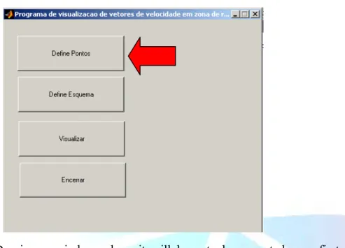
(6) HOLOS Environment, v.9 n.1, 2009 - P. 36 ISSN:1519-8634 (ON-LINE). 1 Pnro point^Xposition in the x axis in centimeters^Yposition in the yaxis^Zpostion in the z axis ANGangle reffering to the horizontal plan or 2 Pnro point^dX or dY or dZ offset in (x,y or z)axis considering a reference point REFPnro reference point or 3 Pnro point^dANGoffset in the reference point direction REFPnro reference point where:. ^ = indicates space bar nro point = number of the point. In the first format, the file name must contain both the coordinate value (x, y and z) for each axis and the angle that the probe has with the horizontal plane. The second format must be renamed taking into account a reference point. Thus, only the linear increment (dx, dy or dz) for each axis in relation to the reference point is set. Finally, the third format should consider only the increment in the probe direction, which is defined by the angle between the probe and the horizontal plane. The angle refers to the down-looking MicroADV model, operating in the vertical position. When the angle is not inputted, zero will be the default. After changing points names with extension VEL, the directory contains the renamed files must be copied to the MatlabR12 6.0 folder in the Work > Veldigital31 directory. The field Current Directory of the MatlabR12 6.0 version must be set to reference the Veldigital31 directory. Later, in the field Command Window, “vel3d” must be used. Thus, the primary window of the visualization program will be opened. This window, from top to bottom, contains four entrance options that must be run in the order that they appear. The operation described in this section was carried out using file with a VEL extension extracted from a real assay. One should choose first the button “Define Points” (Figure 3)..
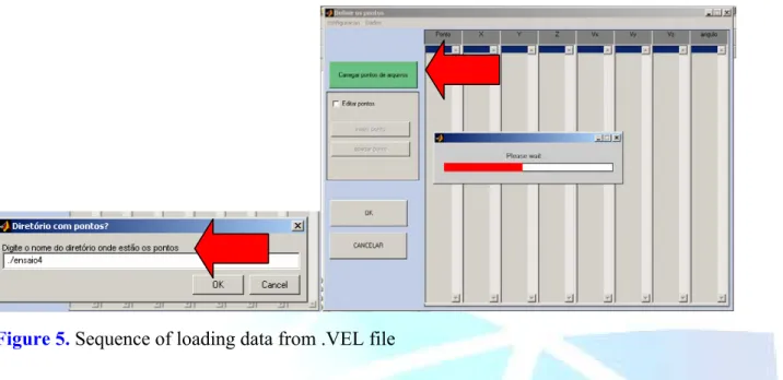
(7) HOLOS Environment, v.9 n.1, 2009 - P. 37 ISSN:1519-8634 (ON-LINE). Figure 3. Veldigital3D primary window where it will have to be executed as a first step for calculation and reading of the resultant vectors.. Continuing, the files that contain the points must be loaded from the directory copied to the folder WORK. Optionally, in the menu Configuration of the tasks bar, the treatment that will be given to the points of the archive (arithmetic mean, geometric and bigger and lesser medium values) can be selected (see Figure 4). Later, one selects the option “To load points of archives”, where the name of the directory that contains the points must be given. The status window then appears, and, in this phase, the grid of points is conferred, and the resultant vectors are calculated. If incorrect points exist (i.e., crossed references, nomination errors, inexistent points, etc.), the information appears in an independent box, and the results are not read or processed. After reading the data, there is an option to invert the axis x and z. Further any tabled value may be added. Figure 5 presents the sequence of some stages described above.. Figure 4. Statistical treatment of the collected data.
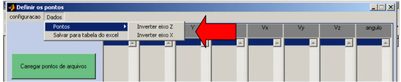
(8) HOLOS Environment, v.9 n.1, 2009 - P. 38 ISSN:1519-8634 (ON-LINE). Figure 5. Sequence of loading data from .VEL file. If there is no problem with the file name, reference, etc., the window containing the loaded points appears in columns containing the point name, coordinates, speed components and collection angle (Figure 6). On the contrary, the type of error appears in a window. In the cases where the adopted origin for the mesh of points does not coincide with the probe orientation, the direction of the axles x and z can be modified (Figure 7). Optionally, the points can be edited by selecting the option “To edit points”. If desired, the points can be confirmed with key “OK”. After this, the primary window appears again, and the second step must be run. The second step is characterized by the scheme definition in which the resultant vectors are plotted. For this propose, the “To define scheme” button must be selected (Figure 8). The drawing must be constructed from the MatlabR12 6.0 tools. The program update must contain the reading of imported data of programs with DWG extension or raster image type.. Figure 6. Loaded points calculated from Figure 4 definition.
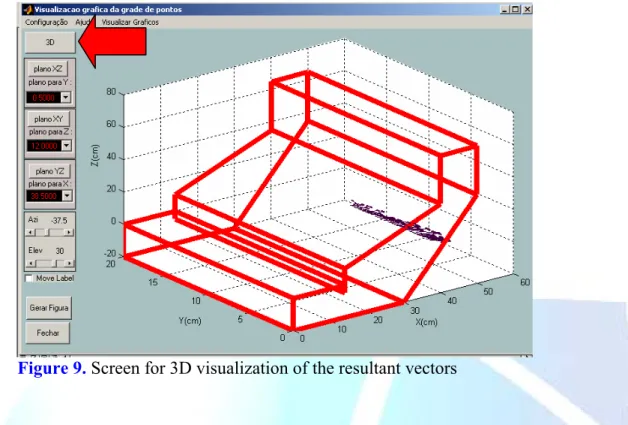
(9) HOLOS Environment, v.9 n.1, 2009 - P. 39 ISSN:1519-8634 (ON-LINE). Figure 7. Axles way inversion according to the probe origin and data acquisition. Then, the visual presentation window is shown (Figure 8). In this window, one must define the drawing and the origin of the adopted net vectors. After the drawing definition (Figure 8a), the origin must be selected by inputting one of the vertices and by choosing the option “To define Origin” (Figure 8b).. a) b) Figure 8. Visual windows for drawing definition in which the resultant vectors are plotted. a) The definition of the scheme. b) The definition of the origin.. The third step consists of vector visualization. For this, the command button “To visualize” in the primary window of the program must be selected. Then, the window shown in Figure 9 appears. In this window, the command button “3D” must be selected so that the vectors can be plotted in the defined scheme..
(10) HOLOS Environment, v.9 n.1, 2009 - P. 40 ISSN:1519-8634 (ON-LINE). Figure 9. Screen for 3D visualization of the resultant vectors. Optionally, the drawing and the vectors can be configured by using the command “Configuration” found in the menu tasks. The scheme can be rotated around the vertical and horizontal axis using the roll bar located on the left. The axis names and positions can also be modified by selecting the option "Move label". From the 3D scheme thus generated, one can produce cuts through different cross sections showing the net defined resultant vectors (Figure 10).. Figure 10. Examples of possible cuts in the vectors net. a) cut in the plan xz; b) cut in the plan xz.. Later, a figure from the 3D scheme can be generated. The MatlabR12 6.0 tools can be also used to modify the characteristics of the figure generated. It is also possible to rotate the scheme around the axis and to magnify some scheme part by choosing the “Zoom” tool (Figure 11)..
(11) HOLOS Environment, v.9 n.1, 2009 - P. 41 ISSN:1519-8634 (ON-LINE). After this, it is necessary to come back to the visualization window to choose the graph format. For this, it is necessary to select the option “To visualize Graphs” in the menu tasks and to indicate the graph type (Figure 12).. Figure 11. Visualization example generated Figure 12. Graph type definition. from the 3D scheme.. Assuming that the surface graph option was chosen, the surface graph that contains the selected region can be plotted (Figure 13). The graph is plotted with differentiated colors in accordance with the intensity of the resultant vectors speed in the direction perpendicular to the selected plan.. Figure 13. Example of surface graph for the plan xy.. Additionally, a border graph can be generated. The border graph presents regions segmented by differentiated colors in accordance with the intensity of the vector component perpendicular to the selected plan (Figure 14). Alternatively, the border graph can be overlapped with the resultant vectors in the associated cut (Figure 15). This alternative supplies a three-dimensional visualization..
(12) HOLOS Environment, v.9 n.1, 2009 - P. 42 ISSN:1519-8634 (ON-LINE). The discussion presented in this paper illustrates one of the possible applications of the VelDigital3D software. It is important to point out that the mesh of points investigated for this illustrative case was intentionally reduced in aims to simplify the operation as our focus was on presenting the functional potential of the program. 4. CONCLUSIONS The Veldigital3D program can be used to assist in the visualization of the data obtained by the probe MicroADV. With the program it is possible to learn about the vectors’ speed distribution in space and to produce different types of graphs, thus constituting a powerful tool for hydrodynamics assessment in many fields of application. The program was designed under the consideration that it be viable in all different areas in which the MicroADV probe is useful. Its conception was based on the search for a simple tool that supplies visual information. The development is inevitably imperfect, and future updates may be required to suit future applications.. Figure 14. Example of border graph produced from Figure 15. Example of overlapping of the the resultant vectors. graphs of border and resultant vectors for plain determined one of interest.. The analysis of the flow conditions using the sounding probe acoustics (ADV) conjugated with the VelDigital3D program have permitted users to learn about the DAF hydrodynamic behavior by means of the three-dimensional visualization in different flow conditions. The graphical user interface developed here is user-friendly and easy to operate. Future versions must consider the code compilation and the algorithm inclusion for raster image insertion. Moreover, similar applications should offer significant assistance in full-scale reactor hydrodynamics analysis..
(13) HOLOS Environment, v.9 n.1, 2009 - P. 43 ISSN:1519-8634 (ON-LINE). 5. ACKNOWLEDGEMENTS The authors are thankful the FAPESP – Fundação de Amparo a Pesquisa do Estado de São Paulo. Foundation of Support to the Research of the State of São Paulo - Brazil for the doctorate scholarship and for the research support that has resulted in the work presented here. This paper was presented in part at the Simposio Internazionale di Ingegneria Sanitaria e Ambientale (SIDISA) in June 2008. LIST OF SYMBOLS 2D two-dimension 3D tree-dimension ADV Acoustic Doppler Velocimeter APC Acoustic Performance Curves cm/s centimeter per second DAF Dissolved Air Flotation DWG AutoCad file extension F dimensionless parameter for turbulence evaluation fr sample frequency fs collection frequency Hz Hertz LDV Laser Doppler Velocimeter m/s meter per second mm/s millimeter per second N number of samples TXT text file extension VEL acoustic file extension Vel3d software executable command 6. REFERENCES GARCÍA, C. M.; CANTERO, M.I.; NNÑO, Y.; GARCÍA, M.H. Acoustic Doppler Velocimeters (ADV) Performance Curves (APCs) sampling the flow turbulence. 2004. Acess in 24 mar. 2004: http://vtchl.uiuc.edu/basic-research/rivers/adv-flowturbulence-pc/apc.pdf LOHRMANN, A.; CABRERA, R.; KRAUS, N. C. Acoustic-Doppler velocimeter (ADV) for laboratory use. Proc. Conf. on Fundamentals and Advancements in Hydraulics Measurements and Experimentation, Buffalo, N.Y, American Society of Civil Engineers, p.351-365. 1994..
(14) HOLOS Environment, v.9 n.1, 2009 - P. 44 ISSN:1519-8634 (ON-LINE). LUNDH, M.; JÖNSSON, L.; DAHLQUIST. J. Experimental studies of the fluid dynamics in the separation zone in dissolved air flotation. Water Research, Amsterdam., v. 34, n. 1, p. 21-30, jan. 2000. SON TEK ADV. Acoustic Doppler velocimeter. Technical documentation. Manual, San Diego, CA, USA 1997. p. 109. VOULGARIS, G.; TROWBRIDGE, J. Evaluation of the acoustic Doppler velocimeter (ADV) for turbulence measurements. Journal of Atmospheric and Oceanic Technology, Washington, DC v.15, p. 272-288. 1998. Manuscrito recebido em: 03/09/2008 Revisado e Aceito em: 21/05/2009.
(15)
Imagem


+5


Documentos relacionados
According to Cañas & Waylen (2012) the survival of catfish species (Pimelodidae) depends on two important displacements during different stages of their life history,
Sem uma análise mais abrangente da GRH, incluindo as diferentes inter-relações entre as práticas (JIANG et al., 2012), e de seus impactos sobre as dimensões do
03.03.02. Na qualidade de proponentes, de membros do Comitê Municipal de Acompanhamento, Controle e Fiscalização da Aplicação da Lei
No caso e x p líc ito da Biblioteca Central da UFPb, ela já vem seguindo diretrizes para a seleção de periódicos desde 1978,, diretrizes essas que valem para os 7
according to their MS 2 fragmentation as different isomers of p-coumaroyl quinic acid. Identities were assigned based on the patterns reported for the caffeoylquinic acid
Peça de mão de alta rotação pneumática com sistema Push Button (botão para remoção de broca), podendo apresentar passagem dupla de ar e acoplamento para engate rápido
Neste trabalho o objetivo central foi a ampliação e adequação do procedimento e programa computacional baseado no programa comercial MSC.PATRAN, para a geração automática de modelos
Ousasse apontar algumas hipóteses para a solução desse problema público a partir do exposto dos autores usados como base para fundamentação teórica, da análise dos dados
