Unconventional Monetary Policy in the Euro Zone

Unconventional Monetary Policy in the Euro Zone

WP15/2015/DE/UECE

_________________________________________________________

W

P

1

Unconventional Monetary Policy in the Euro Zone

John Driffill

Birkbeck College, University of London

16th November 2015

Abstract

The European Central Bank adopted a policy of quantitative easing early in 2015, long after the US and UK, and after implementing a succession of measures to increase liquidity in the Euro zone financial markets, none of which proved sufficient eventually. The paper draws out lessons for the Euro zone from US and UK experience. Numerous event studies have been undertaken to uncover the effects of QE on yields on and prices of financial assets. Estimated effects on long-term government bond yields are then converted into the size of the cut in the policy rate that would normally have been needed to produce them. From these implicit cuts in policy rates, estimates of the effect on GDP and inflation are generated. Euro zone QE appears to have had a much smaller effect on bond yields for the core members states than did QE in the US or UK. Therefore its effects on output and inflation are likely to be proportionately smaller. Its effects on long-term government bond yields in periphery members are greater. QE is compressing interest differential among Euro zone member states. The dangers of QE to which various commentators draw attention, that it creates a danger of inflation in the future, that it creates asset price bubbles, that it allows zombie firms and banks to survive, slowing down the process of adjustment, seem remote. Meanwhile it makes a useful contribution to cutting the costs of debt service and allowing member states more fiscal room for maneouvre.

Keywords: quantitative easing, unconventional monetary policy, Euro zone, financial crisis, European Central Bank

JEL Classification numbers: E31; E43; E51; E58; E63

Acknowledgements

2 Introduction

Quantitative Easing was implemented in the Euro Zone in January 2015. The European Central Bank announced plans to buy at least €1.1 trillion of public sector debt and private sector assets between the start of 2015 and September 2016. It has stated that it may extend the policy if necessary, but may put it on hold if yields on the assets it is attempting to purchase fall below -0.2% per annum, a floor set by the current yield paid on excess bank reserves held at the ECB.

The ECB’s adoption of this policy has been slow in coming. The US Federal Reserve started doing it in late November 2008; the Bank of England in early 2009; and the Bank of Japan resumed QE in 2012, following many earlier policy interventions along similar lines. The ECB’s conversion to QE follows a succession of more cautious interventions.

The context in which they have finally resorted to this measure is the lingering Euro zone recession. Unemployment is falling, but only slowly. The level differs markedly among member states. Growth is weak on the whole. Towards the end of 2014 deflation was looming; inflation dipped into negative territory briefly. Interest rates in several EU members are negative, and the ECB itself is charging banks 0.2% per annum to hold their excess reserves.

To some degree the ECB and other Central Banks are the victims of their own success. Inflation expectations are firmly anchored at or below 2% per annum as a result of the unexpected success of inflation targeting. Giving Central Banks operation (if not total) independence and moving toward the single mandate (of low inflation) has made the commitment to low inflation remarkably credible. Despite the fears of many (including Tim Congdon, a well-known British economist) that the wall of liquidity pumped into the economy would unleash the floodgates of inflation, expectations have not moved. If anything, they have edged downwards over the last few years. The low nominal interest rates prevalent around the world reflect low expected inflation and very low expected future real rates of return.

Real interest rates have been falling for the last three decades. The equilibrium real rate of interest on riskless assets (the rate of return associated with full employment and steady inflation at the target rate of around 2% per annum) now appears to be very low or negative. The question is whether this is temporary or permanent. The secular stagnation hypothesis, that it is permanent, or at least, here for a long time, has gained a lot of traction recently

The combination of low inflation, a long and deep recession and low equilibrium real interest rates has left Central Banks with policy rates at the zero lower bound, unable to reduce them (much) further, and in need of new tools with which to stimulate lethargic economies.

3 The Zero Lower Bound

The re-emergence of Keynes’s liquidity trap has been one of the interesting aspects of the recession. Keynes imagined that nominal interest rates below approximately 2% were unsustainable, believing that the demand for money would become indefinitely large at such a low level of interest rates as bondholders, fearing capital losses on their long bonds, caused by future rises in interest rates, would sell them all and hold bank deposits instead. The Central Bank would be able to buy up all the nominal assets in the economy without being able to push rates all the way down to zero.

However, we have seen rates go all the way to zero and beyond in the last year. The conventional wisdom has been that zero was the lower bound. But the ECB itself now charges banks 0.2% per annum to hold excess reserves. The yield to maturity on 10-year German government bonds fell very close to zero early in 2015. And the central bank of Sweden cut rates to -0.35% in July 2015. There is a sense that the lower bound is now below zero and falling, as central banks test it. Large commercial banks are willing to pay to hold reserves at the Central Bank, rather than holding cash in their vaults, because the storage technology is not costless.

Commentators have at the same time begun to speculate on whether nominal interest rates could be cut further, so that a constant, or even falling, price level need not result in a positive real interest rate. A sufficiently negative nominal interest rate could lead to a zero or negative real interest rate, stimulating the economy even in the face of anticipated deflation. With this in mind, several commentators have considered ending or limiting the use of cash to enforce electronic means of holding money on which a negative interest rate could be imposed. 1

Unconventional policies

It is against this background of below target inflation, high unemployment, weak growth, high public debt, the unavailability of fiscal policy, and nominal interest rates at rock bottom, that central banks

have been using hitherto unconventional policies. “Unconventional” is, of course, arguably a misnomer,

as these policies have become the new conventional.

From all the unconventional things Central Banks might have done, they all have chosen to expand the size of their balance sheets by buying up large amount of public sector debt and private assets with longer maturities. The argument is that while the policy rate directly affects the short end of the maturity spectrum, it has a relatively small and indirect on long-term interest rates, which had remained substantially above short rates, at least until recently.

While there are several channels through which QE might affect the economy, the most widely analyzed (and generally regarded as being important) is the portfolio balance channel. Long-maturity government debt is removed from private sector portfolios and replaced by cash. Were economic agents risk-neutral,

1

Andrew Haldane, writing in the Financial Times, 18th September 2015, “Scrap Cash Altogether, Says Bank of England’s Chief Economist”,

4

and financial markets sufficiently complete and efficient, this substitution would have no effect on real outcomes. If the expectations model of the term structure of interest rates held true, long-term interest rates would continue to be a weighted average of current and expected future short rates. Therefore if the future path of short rates was not affected, long-term interest rates would not be affected either. If however, financial markets are imperfect or incomplete, and agents are not risk-neutral, then a change

in the composition of the private sector’s wealth portfolio may affect relative returns on different assets.

An increase in the quantity of bank deposits held combined with a reduction in the stock of medium- and long-dated government bonds is likely to raise their price, lower returns, and induce substitution towards other assets, such a private sector debt and equity. This effect might be represented as a fall in the term premium on long-dated government debt. 2 The effect the changes in interest rates at the long end of the spectrum is to stimulate investment spending by firms and households and thereby raise real GDP.

A direct effect of QE may in principle come about via banks’ lending, though this has been thought to be

less significant in practice. QE results in the commercial banks holding far more liquid assets in the form of reserves held at the Central Bank than they would have chosen to do. According to the old textbook money multiplier theory of the money supply, banks increase their loans to customers when they have excess reserves, until they are fully loaned up, limited by the amount of reserve assets they can obtain. If this was true in practice, that banks were restrained from lending by the availability of reserves, and

would lend as much possible subject to that constraint, then QE, by increasing the commercial banks’

holdings of reserves, would increase bank loans and the money supply. It is possible that, when interest

rates are stuck at the zero lower bound, there is no further demand for loans and banks’ offers to lend

find no takers. This is the idea that when economic activity is very depressed, attempting to expand the money supply is like pushing on a piece of string, and will be ineffective. In practice the recession has been characterized by very restricted bank lending in many European countries, with banks unwilling to lend despite have large excess reserves, having tightened lending criteria, and at the same time attempting to reduce their leverage and raise their ratio of capital to assets. Capital adequacy has become the operative constraint, not liquidity or reserves.

The Bank of England (Joyce, Tong and Woods, 2011) identifies three further channels of influence of QE: market liquidity; policy signaling; and confidence. In the Bank’s scheme, all five channels directly or indirectly affect asset prices and the exchange rate. Thereby they affect wealth and the cost of borrowing, spending and income, and thus inflation.

A brief review of the macroeconomic context

Policy rates in the United States and the UK were lowered rapidly after the financial crisis. The ECB followed from 2009 onwards, but resisted cutting below 1% until well into 2012, after which they cut them further in steps until late 2014. Japan’s interest rates have been at or near zero since well before the crisis.

2

5

Figure 1 Central Bank Interest Rates

Source of Data: EEAG Report on the European Economy, 2015

Inflation in the Euro zone has fallen consistently since late 2011, and dipped briefly into negative territory early in 2015(figure 2) raising fears that deflation might be about to set in. The ECB monitors data on inflation expectations obtained from surveys and from forward bond yields. The forecast from

Consensus Economics in February 2015 was for inflation below zero in 2015 rising slowly toward ‘just under 2%’ in2018. The ECB’s survey of professional forecasters predicted it rising back to the target in

6 Figure 2 Eurozone inflation

Unemployment has risen since early 2008, when it reached a low point of 7.25%, through the financial crisis to a peak of around 10.25% in early 2010. The early post-crisis efforts to expand demand succeeded in bringing it down again to approximately 9.8% in mid-2011, since when it rose through the public debt crisis to a peak at over 12% in 2013. More recently it has been falling, but only slowly, and was still over 11.25% in the middle of 2015.

7 Figure 3 Euro zone unemployment rate

Figure 4 Euro zone money stock, annual growth rate

8

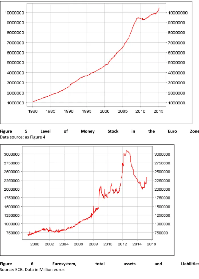
Figure 5 Level of Money Stock in the Euro Zone Data source: as Figure 4

9

Figure 7 Selected Euro zone economies, long-term interest rates

Earlier ECB attempts to increase liquidity in the system are revealed by the data on the Eurosystem’s

10

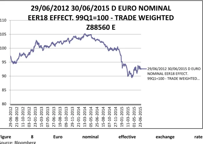
Figure 8 Euro nominal effective exchange rate Source: Bloomberg

As Figure 8 shows, the nominal effective exchange rate of the Euro fell though most of 2014, particularly after June when it started to seem more likely that QE would be undertaken. The dramatic decline occurred in January 2015 around the plans were clearly set out.

The European Central Bank’s Road to Quantitative Easing

The ECB responded to the financial crisis in 2008, and the subsequent banking and public debt crises, with a variety of measures to provide liquidity to the banking system. Long Term Repurchase operations (LTROs) were announced in September 2008, initially with a six month maturity, lengthened to 1 year in May 2009. The programme was phased out in 2010, but reintroduced later. In May 2009 the ESCB announced a Covered Bond Purchase Programme under which they purchased €60 billion of private sector bonds. The ECB attaches great significance to its having moved to a fixed rate full tender allotment procedure. It has widened the range of assets it is willing to accept as collateral when providing liquidity. In May 2010 a Securities Market was introduced, under which LTROs of 3 and 6 month maturities were resumed, the maturity being lengthened to 2 and 3 years in December 2011 and then February 2012, with maturity dates on 29th January 2015 and 26 February 2015. A second covered bond purchase programme, CBPP2, was launched in 2011 running until October 2012.

80 85 90 95 100 105 110 29 -06 -20 12 21 -08 -20 12 11 -10 -20 12 03 -12 -20 12 23 -01 -20 13 15 -03 -20 13 07 -05 -20 13 27 -06 -20 13 19 -08 -20 13 09 -10 -20 13 29 -11 -20 13 21 -01 -20 14 13 -03 -20 14 05 -05 -20 14 25 -06 -20 14 15 -08 -20 14 07 -10 -20 14 27 -11 -20 14 19 -01 -20 15 11 -03 -20 15 01 -05 -20 15 23 -06 -20 15

29/06/2012 30/06/2015 D EURO NOMINAL

EER18 EFFECT. 99Q1=100 - TRADE WEIGHTED

Z88560 E

29/06/2012 30/06/2015 D EURO NOMINAL EER18 EFFECT.

11

None of these programmes was enough to convince the markets that there was no risk of default on the sovereign debt of some of the more problematic member states, Portugal, Spain, Italy, and Greece. Bond yields widened greatly in 2011 and into 2012, as Figure 7 shows. The ECB argued that its policies were not being transmitted effectively into these peripheral countries. Firms, especially small and medium sized enterprises, had to pay much higher rates for bank loans and the supply of loans was highly restricted. Banks were rationing credit, as they de-leveraged, and tried to raise their capital ratios.

Consequently, the ECB announced more radical measures, In August and September 2012 the ECB set out its plans for ‘Outright Monetary Transactions (OMTs), under which it would buy the debt of problem states on secondary markets, in principle without limit. This turned out to be the long-awaited ‘bog

bazooka’ that calmed markets without any need for any actual ECB bond-buying. The commitment alone

was enough. Yield spreads fell markedly. This was followed in June 2014 by the announcement of targeted long-term repurchase operations, to run for two years. They were conducted in September and

December 2014 and will mature in 2018. Finally, the package known as ‘quantitative easing’ was

announced: the Enhanced Asset Purchase Programme, including the Asset Backed Securities Purchase Programme (ABSPP) announced in September 2014, a third covered bonds purchase programme started 21 Nov 2014, and a public sector purchase programme (PSPP), which was intended to start on 9th March 2015.

Quantitative Easing in the United States

Quantitative Easing in the United States began in late November 2008 (“QE1”), when the Federal Reserve started buying $600 billion in mortgage-backed securities. By March 2009, it held $1.75 trillion of bank debt, mortgage-backed securities, and Treasury notes. This stock reached a peak of $2.1 trillion in June 2010. Further purchases were halted as the economy started to improve, but resumed in August 2010 when the Fed decided the economy was not growing robustly. After the halt in June, holdings started falling naturally as debt matured and were projected to fall to $1.7 trillion by 2012. The Fed's revised goal became to keep holdings at $2.054 trillion. To maintain that level, the Fed bought $30 billion in two- to ten-year Treasury notes every month.

In November 2010, the Fed announced a second round of quantitative easing, QE2, buying $600 billion of Treasury securities by the end of the second quarter of 2011. A third round of quantitative easing, "QE3", was announced on 13 September 2012. It included a new $40 billion per month, open-ended bond purchasing program of agency mortgage-backed securities. Additionally, the Federal Open Market Committee (FOMC) announced that it would probably keep the federal funds rate close to zero "at least through 2015." On 12th December 2012, the FOMC announced an increase in the amount of open-ended purchases from $40 billion to $85 billion per month.

12

from $85 billion to $65 billion a month during the September 2013 policy meeting and the bond-buying programme might end by mid-2014. Bernanke suggested that if inflation followed a 2% target rate and unemployment decreased to 6.5%, the Fed would likely start raising rates. The stock markets dropped by approximately 4.3% over the three trading days following the announcement. On 18 September 2013, the Fed decided to hold off the scaling back of its bond-buying program and began tapering purchases the next year, in February 2014 Purchases were halted on 29 October 2014, after the Fed had accumulated $4.5 trillion in assets.

Quantitative Easing in the UK

The Bank of England’s Monetary Policy Committee (MPC) cut interest rates by 3 percentage points during 2008 Q4 and another 1.5 percentage points in early 2009, taking Bank Rate down to 0.5% by March 2009. Nevertheless, it was felt that more was needed, and MPC announced a programme of large-scale purchases of public and private assets using central bank money, with aim of injecting money into the economy and boosting nominal spending and help achieve the inflation target. As Joyce, Tong and Woods (2011) note, “Between March 2009 and January 2010, the Bank purchased £200 billion of assets, mostly medium and long-dated gilts. These asset purchases represented nearly 30% of the amount of outstanding gilts held by the private sector at the time and around 14% of annual nominal GDP. Combined with earlier liquidity support measures to the banking sector, these purchases increased

the size of the Bank’s balance sheet relative to GDP threefold compared with the pre-crisis period.” Since then the size of the programme has been increased several times. In November 2009, the Monetary Policy Committee (MPC) voted to increase total asset purchases to £200 billion. Most of the assets purchased were UK government securities. The Bank has also purchased smaller quantities of high-quality private-sector assets. In October 2011, the Bank of England announced that there would be another round of QE, in which it would buy £75 billion of assets. In February 2012 a further £50 billion round of QE was announced. And in July 2012 the Bank announced that another £50 billion would be purchased, bringing the total amount to £375 billion.

Effects of QE in the US

An early and widely cited study of QE in the United States, by Gagnon, Raskin, Remache and Sack (2010) focused on the effects of QE on the portfolio of assets held by the private sector, on the changes in yields of alternative assets that this brought about, and the consequent changes in aggregate spending. They used a mixture of event studies and regression analysis. Other things being equal, the impact effect of QE is to reduce the quantity of medium and and long term bonds held by the private sector, replacing them with bank deposits, while the commercial banks hold more reserves at the central bank and their customers have more deposits with them. This portfolio shift lowers risk premium on long term government bonds, independently of the expected future path of short rates.

13

Chairman, statements by the FOMC, and release of Minutes from FOMC meetings. The argument for this procedure is that within these windows, most of the change is due to the announcement about QE, and that the change is highly persistent. Adding up all the separate changes gives a good estimate of the cumulative effect of all the announcements relating to QE over the period between 25th November 2008 and 28th January 2010. The effect ranges from -19 basis points for 2-year US Treasury bonds when an extended set of events is used, to -156 basis points for 10-year Agency bonds, when the baseline event set is used. Table 1 summarizes the findings of Gagnon et al (2010), showing the variety of effects for different instruments and event sets.

2 year US Treasuries

10 year US Treasuries 10-year Agency Agency Mortgage-Backed Securities

10 year TP 10-year Swaps

Baa Index (Corporate Bonds)

Baseline Event Set

-34 -91 -156 -113 -71 -101 -67

Extended Event set

-19 -62 -140 -123 -50 -83 -74

Cumulative change between 24 Nov 2008 and 28 Jan 2010

-39 30 -96 -109 21 20 -482

Table 1 Interest Rate Changes for various instruments, in windows around key QE announcements in the US between 25 Nov 2008 and 28 January 2010 Source of data: taken from Table 1 of Gagnon et al (2010)

Gagnon et al further investigated the effects of QE using a variety of regression models for the term premium on 10-year bonds. They found an effect of 51 basis points (with a 95% confidence interval from 31 to 74) on unadjusted data and 38 basis points (with a 95% confidence interval from 22 to 54) on a duration-adjusted data, using an OLS regression; they find corresponding effects of 50 basis points (95% confidence interval 31 to 69) on unadjusted data and 36 basis points (95% confidence interval from 20 to 53) on duration-adjusted data, using a dynamic OLS regression. An alternative yield level model vies point estimates of 82 basis points (confidence interval from 50 to 115) on unadjusted data and 58 (with confidence interval 31 to 84) on duration adjusted data. These results suggest a clearly negative effect on the 10-year term premium, though with wide margins or error.

Krishnamurthy and Vissing-Jorgensen (2011) have dissected the effects of QE on markets around the dates of key events in more detail to uncover the channels of influence on different markets. They argue that purchases of different assets affect different markets through different channels. A liquidity channel raises the yield on US treasury bonds by increasing the amount of liquidity, in the form of bank reserves, in the system. A safety channel exists because there is a clientele for very safe assets; it lowers

14

mortgage backed securities, and when QE buys up these assets, the premium due to prepayment risk falls, and prices of these assets rise. A default risk channel works on the risk premium on risky bonds. When the supply of these is reduced by QE, their yield goes down and price goes up. Finally, the inflation channel works through QE’s raising expected future inflation, and raising uncertainty about future interest rates. They argue that all these have played a role to varying degrees in the US’s first and second rounds of QE.

The effect of QE on term premiums is only the first element in an estimation of its effect on output and inflation. The analysis has continued by estimating how big an effect the cut in term premiums might have on aggregate demand and inflation. Again, this has been done indirectly in many cases, first asking what fall in the policy rate would produce the estimated fall in the long rate, and then asking what would the effect on aggregate demand and inflation of this fall in the policy rate have been. D’Amico et al (2012) find that QE1 in the US reduced long rates by 25 basis points, and QE2 by 45 basis points. They report estimates that in the recent past a fall of 25 basis points in long rates was produced by a 100 basis point fall in the policy rate. Therefore they argue that QE1 was equivalent to a 140 b. p. cut in the policy rate, and QE2 to a 180 b. p. cut, and therefore argue that QE had substantial effects.

Empirical estimates of effects of QE in the UK

Studies similar to that of Gagnon et al (2010) have been carried out for the UK. The first rounds of QE were implemented in 2009 and 2010, and a series of announcements were made by the Bank of England and the government from 19th January 2009 onwards. In the days surrounding these announcements, as reported by Joyce, Tong and Woods (2011), there were substantial falls in yields, particularly in March 2009 when QE was first implemented. The cumulative effect, adding up changes around key events between January 2009 and February 2010, is estimated as a fall of just under 100 basis points in the yield on UK government bond yields.3

As in the US, the next step in the analysis is to work out how big an effect on aggregate demand and inflation such a cut in bond yields would have. Joyce, Tong and Woods (2011) describe this as a ‘bottom

-up approach’. They note that “Ideally one would want to make an assessment using a properly specified

structural model. But no such model embodying all the relevant transmission channels discussed earlier appears to exist. The forecasting model used by the Bank of England, in common with most large-scale macroeconomic models, does not explain risk premia and therefore does not embody a portfolio

balance channel.” Therefore the job of working out the effect of QE on GDP and inflation consists of two parts: firstly the impact of asset purchases on gilt prices and other asset prices; and secondly the effect of asset prices on demand and inflation.

Structural vector auto-regressions (SVARs) can be used to determine the effects of bond yields on demand and inflation. In exercises reported by Joyce, Tong and Woods (2011) an SVAR, in which the variables are the policy rate, the government bond yield (the ten-year spot rate), real GDP growth and

3

15

CPI inflation, is estimated over the period from the 1st quarter of 1992to the 2nd quarter of 2007. A ‘QE

shock’ is identified as a negative shock to bond yields that leads to a contemporaneous rise in GDP and CPI points, is estimated to result in a peak impact on the level of real GDP of just under 1.5% and a peak effect on annual CPI inflation of about 3/4 percentage points. The authors remark that “These effects should be taken as illustrative, given the simplicity of the model and the fact that it has been estimated on a sample predating the crisis.”

As an alternative to SVARs, Kapetanios et al (2011) have estimated three different time-series models of varying complexity, and used them to produce counterfactual forecasts of the effects of QE. Averaging across the models suggests a peak effect on GDP around 1½% and peak effect on CPI inflation of 1½ percentage points. Once again, the estimates vary considerably across the individual model specifications, and with the assumptions made to generate the counterfactual forecasts, suggesting they are all subject to considerable uncertainty.

A third line of attack essayed by Bridges and Thomas (2012) uses a ‘monetary approach’ in which they examine the impact of QE on the money supply. These estimated impacts are then applied to two econometric models, one an aggregate SVAR model, a second a linked set of sectoral money demand systems. From these they calculate how asset prices and spending need to adjust to make money demand consistent with the increase in broad money supply. Their preferred results suggest that higher money supply due to QE boosted GDP by around 2% and CPI inflation by about 1%. Once again, these estimates are subject to a lot of uncertainty.

Despite the frequently mentioned large margins of error surrounding these estimates, it is striking that the orders of magnitude of effects on GDP and inflation are common to all these studies.

Despite the apparent unanimity among empiricists and econometricians, not everyone is so sanguine about QE. Chen et al (2012) simulate the Federal Reserve second Large-Scale Asset Purchase program (QE2) in a dynamic stochastic general equilibrium (DSGE) model, the parameters of which have been estimated on US data. They assume bond market segmentation to replicate the idea of the ‘preferred habitat model of the term structure. That is, bonds of different maturities are assumed not to be perfect substitutes. Different investors have preferences for bonds of different maturities, and are willing to hold bonds of other maturities if compensated by higher expected returns. Despite this assumption, they find that GDP growth increases by less than a third of a percentage point and inflation barely changes, relative to what happens in the absence of QE. Their findings emerge because, on their estimates, the elasticity of the risk premium to the quantity of long-term debt is small, as is the degree of financial market segmentation. They find that without a commitment to keep the nominal interest rate at its lower bound for an extended period, the effects of the US’s asset purchase programs would be even smaller.

16

(and a liquidity crisis) based on work of Kiyotaki and Moore (2012). In this they assume that a liquidity crisis, such as happened in 2008 and 2009 following the collapse of Lehmann Brothers, when many assets became illiquid because no-one would buy them and no-one was able to trade them, is countered by the central bank stepping in an buying up illiquid assets and replacing them with highly liquid ones, such as Central Bank reserves. This they show can have very powerful effects on the real economy. Driffill and Miller (2013) develop variants on the theme of Kiyotaki and Moore (2012), introducing downward rigidity of wages and prices, and, using a smaller model than Del Negro et al, show that this type of intervention has strong effects.

A sketch event study of QE in the Eurozone

By analogy with the studies of QE in the UK and UK, one might consider key dates in the introduction of the policy in the Eurozone, when announcements were made or actions taken, and examine the changes in prices of and yields on assets in narrow windows around those dates. The following dates stand out:

• 5 June 2014: the ECB announces TLTROs (targeted long-term repurchase operations) and preparatory work on ABS (asset backed securities) purchases

• 22 August 2014: the ECB President, Mario Draghi, makes a speech at Jackson Hole, in which he links the need for monetary and fiscal policies to stimulate aggregate demand with policies aimed at achieving structural change

• 18 Sept 2014: Mario Draghi makes a speech to the European Parliament Economic and Monetary Affairs committee

• 22 January 2015: the ECB announces the expanded asset purchase (QE) programme

• 9 March 2015 – the beginning of QE programme

Date Germany France Portugal Greece

4th June 2014 -0.57 -7.00 1.97 15.39

22nd August 2014 -0.30 9.00 18.99 11.73

18 September 2014 0.93 -2.00 0.83 -0.98

22nd January 2015 13.90 14.00 31.66 73.19

17

Total 23.20 15.00 57.75 5.06

Table 2 Fall in 10-year Government bond yields around dates of key QE announcements Data source: Datastream. Units of measurement: basis points. Daily observations, using a 1-day window

around announcements

The changes in in bond yields in the Euro zone economies are strikingly smaller than they were in the US and UK in 2008, 2009 and 2010, and also they are diverse. Yields fell modestly in Germany and France, the member states with the lowest rates. Portuguese yields fell more (57.75 basis points), perhaps because Portuguese financial markets will benefit more from the extra liquidity provided by QE; Portuguese government bonds will be included in the programme; it will reduce risk premiums on them; the Portuguese economy will benefit greatly from any macroeconomic stimulus it gives. Greek bond yields hardly moved in response to QE; they were dominated by political changes in Greece and

negotiations with the Troika or ‘the institutions’ in 2015. In the case of Germany and France, the largest effect was produced by the announcement of the details of QE on 22nd January 2015. The second largest in Germany followed the actual implementation on 9th March 2015; the second largest in France

followed Draghi’s speech at Jackson Hole is August 2014, perhaps because the linkage that he made between structural reform and macroeconomic stimulus is more important in France, where the perceived need for structural reform is greater, than in Germany.

This event study confirms the view that Eurozone QE is likely to have weaker effects than it had in either the US or UK.

A back-of the-envelope calculation

Despite indications that Eurozone QE may be less effective than either in the US or UK, it may be of interest to calculate how large a proportionate effect would be, to give an upper bound estimate.

In the UK, the Bank of England bought £200bn of assets by late 2011. At the time the GDP of the UK was approximately £1.6 trillion, the money stock (M3) £2.23 trillion, and general government debt £1.32 trillion. The estimated effect of QE on real GDP has been put in the range of 1.5% to 2% and the effect on inflation between 0.75% and 1.5%.

In the Eurozone, asset purchases of €1.1 trillion are planned; Eurozone GDP is of the order of €10 trillion; general government debt stands at approximately €9 trillion; and the money stock (M3) is €10.4 trillion.

18

In view of the much lower riskless long-term nominal interest rates in the Euro zone at the time of the introduction of QE, as compared with the UK, this may be regarded as an optimistic view of the likely effects.

More radical policies

Among the criticisms of QE is that it has been too conservative a policy, in that it swaps one highly liquid asset (public debt) for another (central bank reserves). Consequently the effects on interest rates, aggregate spending and inflation have been modest. Some commentators have called for more radical and adventurous policies.

One such, sometimes described as ‘credit easing’, has the central bank buying riskier private sector

assets, such as corporate bonds or equity, a policy modeled by Kiyotaki and Moore (2012) and Driffill and Miller (2012). This would switch the private sector’s asset portfolio away from risky long-term and illiquid assets towards safe, short-term, liquid assets. Central banks have on the whole refused to engage in this activity, on the grounds that it further blurs the boundaries between monetary and fiscal policies. The distribution of equity and corporate debt purchases across different sectors of the economy is potentially a politically sensitive decision. There is concern that it exposes the balance sheet of the central bank to unacceptably high risk.

There is still a question of whether it would be more effective than QE as currently practiced. The change in the portfolio of risk and return of the private sector is matched by a corresponding change in the opposite direction by the public sector (here consolidating the central bank with the rest of the public sector). Private sector agents would be able to insulate themselves from the effects of these shifts by holding a suitable mix of private and public sector assets and liabilities.

Some commentators have suggested even more radical policies. At the height of the financial crisis,

Adam Posen, then a member of the Bank of England’s Monetary Policy Committee advocated setting up a public investment bank, which would undertake direct lending. Effectively the government and central bank would be lending to firms, whose access has been limited by banks’ attempts to recapitalize and reduce risk.4 Banks are charged with having been excessively conservative, and arguably should have been bypassed.

Conclusions

Quantitative easing in the US and UK appears to have had modest beneficial effects: a small increase in the level of GDP, of the order of 0.75 to 1.5%, and a small increase in the price level, of a similar order, relative to what they would otherwise have been. Long run interest rates have been brought down a little; estimates suggest by 1 percentage point or less. The effects appear to have come mainly through shifts in portfolios, and prices of and yields on assets, rather than by stimulating banks to lend more.

4_{Speech given in Gloucestershire, 13 September 2011, “How to do more”, was accessed on 14 Nov 2015 from}

19

By the time of the introduction of QE in the Euro zone, ten-year government bond rates in Germany and other Euro zone members, to whose debt the markets assigned no default risk, had fallen to 1% or less, and the scope for QE to induce further falls was limited. But QE may have brought about a more pronounced lowering of bond yields in troubled economies such as Portugal. QE is very probably contributing to narrowing the spread of bond yields across the Euro zone. Furthermore, announcements made during 2014 of plans for QE in 2015 were accompanied by significant falls in the Euro exchange rate.

In the UK, the initial rounds of QE seem to have lowered long-term government bond yields by around 100 basis points, on the basis of event studies. In the Euro zone, announcements about QE in 2014 and 2015 appear to have brought down ten-year bond yields in core members by 23 basis points (Germany) and 15 basis points (France), but 57 basis points in Portugal, giving weight to the view that the effect on riskless long-term bond yields has been small, but that QE is compressing differentials between member states.

There are several aspects of QE that have not been the focus of this paper. Many commentators express fears that QE may bring a risk of inflation in the future, when demand increases and banks may be able to mobilize the excess liquidity in the system (in the form of excess central bank reserves which they are holding). This seems a remote prospect, as the Central Bank will have time to raise the policy rate and reverse the asset sales to remove liquidity, before inflation can take off. While there may be a risk that the Central Bank makes losses on asset sales (having bought assets at high prices and low yields, later having to sell them off at lower prices and higher yields), these losses should be set against the substantial profits central banks have been making in recent years while they have been holding interest bearing government debt with low, zero, or even negative interest-bearing reserves as the counterpart liabilities. The profits of the Central Banks arising from QE are returned to governments. By holding down long-term government bond yields, and by effectively funding a large fraction of the public debt with central bank reserves, QE usefully cuts the burden of servicing the public debt and eases the government budget constraint.

Some commentators are concerned that QE has sustained bubbles in asset prices. There is anxiety about the UK housing market, for example. But higher asset prices, which increase private sector wealth, are one of the routes through which QE works. There has been little evidence to date of bubbles forming.

Another criticism of QE is that it keeps alive ‘zombie’ firms and banks, and slows down the restructuring

of the economy. Again, this seems to be misunderstanding. QE is intended to allow slower adjustment,

inter alia giving banks longer to rebuild their balance sheets, and mitigating unemployment.

20 References

Bridges, Jonathan, and Ryland Thomas (2012), “The impact of QE on the UK economy — some

supportive monetarist arithmetic,” Bank of England Working Paper No. 442, accessed on 15 November 2015 from http://www.bankofengland.co.uk/research/Documents/workingpapers/2012/wp442.pdf

Chen, Han, Vasco Curdia, and Andrea Ferrero, (2012) “The Macroeconomic Effects of Large-Scale Asset Purchase Programs,” Economic Journal, Volume 122, Issue 564, pp. F289–F315

D’Amico, S., English, W., Lopez-Salido, D., and Nelson, E. (2012) The Federal Reserve’s Large-Scale Asset Purchase Programs: Rationale and Effects, Economic Journal, vol. 122, pp. F415-F446

Del Negro, M., Eggertsson, G., Ferrero, A., and Kiyotaki, N. (2011) The Great Escape? A Quantitative Evaluation of the Fed's Liquidity Facilities, Federal Reserve Bank of New York, Staff Report 520

Driffill, John and Marcus Miller, “Liquidity when it matters: QE and Tobin’s q”, Oxford Economic Papers, 2013

Gagnon, J., Raskin, M., Remache, J., and Sack, B. (2010) Large-scale asset purcahses by the Federal Reserve: Did they work? Federal Reserve Bank of New York, Staff Report 441

Gertler, M. and Karadi, P. (2011) A model of unconventional monetary policy, Journal of Monetary Economics, 58, 17-34

Joyce, M., Tong, M., and Woods, R. (2011) The United Kingdom’s Quantitative Easing Policy: Design, Operation and Impact, Bank of England Quarterly Bulletin, 3, 200-212

Joyce, M., Lasaosa, A., Stevens, I., and Tong, M. (2011) The Financial Market impact of Quantitative Easing in the United Kingdom, International Journal of Central Banking, 7, 113-161.

Kapetanios, G., Mumtaz, H., Stevens, I. and Theodoridis, K. (2012), “Assessing the Economy-wide Effects of Quantitative Easing,” Economic Journal, vol. 122, pp. F316–F347

Kiyotaki, N. and Moore, J. (2012) Liquidity, Business Cycles, and Monetary Policy, NBER Working Paper 17934.

Krishnamurthy, A. and Vissing-Jorgensen, A. (2011) “The effects of quantitative easing on interest rates: channels and implications for policy”, Brooking Papers on Economic Activity, fall, pp. 215-265

Vayanos, Dimitri, and Jean-Luc Vila, 2009, “A Preferred-Habitat Model of the Term Structure of Interest